Effectiveness of Machine-Learning and Deep-Learning Strategies for the Classification of Heat Treatments Applied to Low-Carbon Steels Based on Microstructural Analysis

Featured Application

A support tool for the image recognition of microstructures for quality control in carbon-steel manufacturing.

Abstract

This work aims to compare the effectiveness of different machine-learning techniques for the image classification of steel microstructures. For this, we use a set of samples of hypoeutectoid steels subjected to three heat treatments: annealing, quenching and quenching with tempering. Logically, the samples contain the typical constituents expected, and these are different for each treatment. Images are obtained by optical microscopy at 400× magnification and from different low-carbon steels to generate the data with some heterogeneity. Learning models are created with an image dataset for classification into three classes based on the respective heat treatments. Likewise, we develop two kinds of models by using, on the one hand, classical machine-learning methods based on the “bag of features” technique and, on the other hand, convolutional neural networks (CNN) with a transfer-learning approach by using GoogLeNet and ResNet50. We demonstrate the superiority of deep-learning techniques (CNN) over classical machine-learning methods.

1. Introduction

In recent years, different investigations have been conducted on the identification and classification of material microstructures. Studies can be found with different approaches and results based on classical machine-learning algorithms and neural networks applied to optical microscopy analysis or SEM images. The random forest technique is used as the base algorithm to obtain classifiers in the experiments performed. Thus, Bulgarevich et al. [1] developed an analysis of steel images and classified ferrite–pearlite, ferrite–pearlite–bainite and bainite–martensite microstructures. In a subsequent publication, [2], the selection of models was improved by extracting different statistical attributes from the dataset, thereby, obtaining a precision of 90%.

Muller et al. [3] studied the classification by using a support vector machine algorithm, SVM, of pearlite, martensite, transformed pearlite, debris of cementite, residual austenite and upper and lower bainite by using SEM images. Their results showed an acceptable accuracy of 82%. They also implemented an inference method for obtaining the area (%) that the corresponding phase occupies, finding, by the end of the experiment, an accuracy of 89%.

Other studies have directly addressed the problem of image segmentation with an optical image dataset. Thus, Kim et al. [4] identified ferrite, pearlite and martensite by using a convolutional neural network, CNN, to obtain parameters and the simple linear iterative clustering algorithm, SLIC, for segmentation. They achieved efficient performance. Other approaches to the classification problem can be found from images taken from optical microscopy. Nishiura et al. [5] investigated a system for automatically estimating the steel quality level with a model based on the VGG16 neural network [6] and obtained a success rate of 92.5%.

Regarding datasets that consist of images obtained with an electronic microscope (SEM, EBSD), several works can be found, such as Tsutsui et al. [5], where kernel-averaged misorientations were used as parameters to classify bainite and martensite with the classical SVM and random-forest algorithms, achieving acceptable results. Different works with these types of images have created models with deep-learning techniques, such as that of Maemura et al. [7] where eight types of steel microstructures were classified: upper bainite, martensite and their hybrid structures. They used the pre-trained network ResNet50 as a classifier, obtaining accuracies of up to 97% using a voting method to analyze the results by means of a local interpretable model-agnostic explanation, LIME.

Zhu et al. [8] established a comparative method of two algorithms for feature extraction, one with VGG16 pre-trained with ImageNet and another one with a gray-level co-occurrence matrix, GLCM. They concluded that the best combination for classification was VGG16 as a feature extractor with an SVM classifier. In this case, their research was applied to hot stamping ultra-high-strength steels.

A segmentation technique with electronic images was addressed by Motyl et al. [9], where, through the use of U-NET [10], they searched for the detection of pearlite islands in biphasic ferrite–pearlite steels, reaching estimates between 79% for EBSD images and 87% for SEM images. Likewise, Breumier et al. [11] dealt with the subject of segmentation with U-NET; however, in this case, the different constituents involved were identified using the band contrast, BC, grain boundary misorientations and kernel average misorientation (KAM) maps.

De-Cost et al. [12] researched a different approach to steel image segmentation by working with the VGG16 pre-trained network and PixelNet [13] over the Ultra High Carbon Steel Dataset [14]. Rather than training two separate CNNs, they demonstrated that introducing a single CNN in a multi-task setting was more appropriate. Thus, microstructures were mapped to a common numerical representation before the corresponding classification of microconstituents.

Other investigations approached the recognition of microstructures from the point of view of the inference of material properties, as in the case of Wang et al. [15,16], where steel properties, such as the stress–strain behavior, and particularly, the UTS and the total elongation, were obtained from micrographs of different steels using deep-learning techniques.

Many papers have tackled classification problems using deep-learning and traditional machine-learning approaches, in different contexts for performance comparison. Dhola et al. [17] used deep learning for sentiment analysis and showed better accuracy compared with traditional machine-learning models. Other studies, such as Wang et al. [18], evaluated SVM and a narrow CNN (two dense layers) for two different datasets, and they concluded that, for a large dataset (MNIST) the deep-learning approach performed better than traditional ML; however, when using a small sample dataset (COREL1000), the accuracy of SVM was slightly better than the CNN.

Amri et al. [19] reviewed the effects of imbalanced data disparity with a MINST handwritten dataset. In the experiments, a deep belief network (DBN) is used, and the results were compared with conventional ML algorithms, such as backpropagation neural network, SVM, decision trees and naïve Bayes. This research concluded that DBN achieved a high accuracy rate and low error according to the performance metrics as compared to the other ML algorithms, which are more affected by data imbalance.

As seen so far, there are several ways to approach the classification of steel microstructures using machine-learning models. Each research work proposes one or several models with different levels of success. However, it is difficult to determine the best algorithm to be used with steel microstructures because the data are obtained with different technologies (optical or electronic) and are not sufficiently extensive and homogeneous to create models that manage to generalize the predictions and avoid overfitting. In this work, we take into consideration optical images and compare classical and deep-learning models to obtain the best strategy to be established as a starting point for future research.

Thus, the present work aims to perform experiments for creating different models generated by supervised machine-learning techniques to classify the microstructures of steels that have been subjected to several thermal treatments. We create our dataset based on previously labeled steel microstructures, and all the images are taken using optical microscopy. The experiments are on the one hand, based on six classic machine-learning (ML) algorithms and, on the other hand, by working with a transfer learning scheme based on the deep-learning networks “GoogLeNet” and “ResNet50”.

The images for creating the machine-learning models were obtained from three sets of hypoeutectoid carbon steel specimens subjected to annealing, quenching and quenching plus tempering heat treatments. Image classification was performed for the three categories, one for each heat treatment, based on the hypothesis that each treatment has a characteristic microstructure.

2. Materials and Methods

2.1. Steel Samples and Image Data Setting

Low-carbon steels subjected to different heat treatments were considered, and the chemical compositions are indicated in

Table 1. Chemical composition (weight %) of low-carbon steel samples according to ISO 683-1:2019 and ISO 683-2:2019 standards. Number of samples for each heat treatment: annealing (A), quenching (Q) and tempering (T).

Steel	Samples	Chemical Composition Weight %
		Mo	Si	Mn	P	S	Cr	Mo	Ni
C22E	0A 1Q 0T	0.17		0.6
C45E	4A 1Q 2T	0.45		0.65
37Cr4	1A 1Q 2T	0.37		0.75			1.05
34CrMo4	1A 0Q 0T	0.35		0.75			1.05
40NiCrMo6	0A 1Q 1T	0.4		0.7			0.8	0.25	1.8

.

Metallographic samples were investigated by the authors for this research, according to well-established procedures. In this way, no adversarial attacks are expected regarding model creation [20].

These steels can present different microstructures depending on the type of heat treatment that has been undergone. In the case of annealing, the observable microconstituents are ferrite and pearlite. Martensite is the dominating phase that appears after quenching. Depending on the steel composition, some minor quantities of retained austenite can appear. Tempering after quenching provides different microstructures depending on the temperature; however, for tempering at intermediate temperature, the typical microstructure is composed by tempered martensite that is contoured with a thick coating of precipitated cementite. For annealing, quenching and quenching–tempering, other constituents than those mentioned can appear depending on the steel composition and the way in which the heat treatment is performed. In Figure 1, Figure 2 and Figure 3, representative microstructures corresponding to some of the experimented steels are shown. All the steel samples were prepared for the optical microanalysis at 400×, which was performed using an inverse microscope Nikon equipped with a Nikon FX-35WA camera.

This procedure permitted digital images to be taken at a resolution of 2080 × 1542 pixels. Optical microscopy under those conditions is a typical microstructure characterization technique. Steel microstructures were selected taking into consideration several criteria. Although the expected microstructures should be similar in all steels, some heterogeneities can be considered. In Figure 1a, we observe perlite (dark areas) and ferrite (white areas) as the typical constituents of an annealing structure of a low-carbon steel. Perlite is a lamellar structure of alternative bands of ferrite and cementite; however, for many islands of perlite, this structure cannot be resolved due to the microscope augmentation, and these islands appear as dark areas.

This lack of uniformity of perlite is due to the fact that annealing is performed with a progressive cooling, and the temperatures at which perlite is formed are not uniform in all areas of the piece. In addition, the different plane orientation of the perlite respect to the observation one, led to a different appearance of this constituent. The microstructure of Figure 1b presents a similar aspect to Figure 1a but with a different perlite–ferrite proportion. In Figure 1c, a very fine troostitic perlite can be observed. Finally, Figure 1c corresponds to an annealing treatment for which only ferrite and cementite appear, since perlite was transformed into these two phases. Nevertheless, we can suppose that the isles of perlite are a consequence of the difficulties of atomic migration in solid state, i.e., diffusion phenomenon.

Figure 2 corresponds to microstructures of quenching, that is, the predominant constituent is martensite; however, again, some differences exist between them. The most typical microstructures are those corresponding to Figure 2b–d. In these structures, bainite frequently appears in low proportion, and it is difficult to identify it. However, even in these cases, martensite can be colored in a different way. Thus, the clear areas in the microstructures along with the dark ones of Figure 2b–d are martensite.

Sometimes, the general aspect of the micrograph can be changed by using, for example, an optical filter, as seen in Figure 2b, which includes this effect in the machine-learning techniques experimented herein. Finally, Figure 2a corresponds to an incomplete quenching of a low-carbon steel. Due to that, although the predominant phase is martensite, some other constituents exist, notably ferrite, and it is clear that the visual aspect of this micrograph is somewhat different to the rest of them.

Figure 3 presents typical microstructures of quenching and tempering at medium temperature, Figure 3a–c, and at high temperature, Figure 3d. Tempering at low temperatures was discarded because the microstructure is so similar to the quenching one, that it is typically necessary to support the microstructural analysis with other techniques. For an intermediate tempering treatment, at 400–500 °C, the steel microstructure is characterized by the transformation of martensite into what is usually called tempered martensite.

This new constituent consists of cementite precipitation into a ferrite matrix that adopts the shape of a thick continuous coating contouring the antique martensite borders. If tempering is performed at high temperature, 600 °C, martensite decomposes to ferrite, and cementite appears as a globular precipitate. Nevertheless, considering again the limitations of atomic migration in these processes, the structure is characteristic and presents differences with those obtained in other heat treatments; however, visually, some affinities can be observed to those corresponding to the intermediate tempering.

Different steels and microstructures were selected in order to introduce some degree of heterogeneity to the classification techniques to be considered in the present work. For each of the samples indicated in Table 1, ten different pictures were obtained. This means that, for each steel, we randomized selected different microstructural areas, attempting to consider, as much as possible, the heterogeneities existing in the corresponding steel, while avoiding overlapping of the characteristic features involved. To reinforce this effect, in some cases, several different samples were considered, i.e., C45E and 37Cr4 steels.

To sum up, an image dataset was created composed of 80 images for annealing, 40 for quenching and 50 for quenching and tempering samples. Nevertheless, the number of images for each class in the datasets should be balanced to improve the machine-learning performance. Thus, to match and extend the amount of data and to fit the transfer-learning network requirements, the original 2080 × 1542-pixel images were cropped.

At this point, the question was which resolution to choose for cropping the images. If images were split up in a low-resolution range, the performance time in Classic ML algorithms would significantly increase. However, in that case, a high number of files would be disposed of in the input training, which is suitable for deep learning [21,22,23,24,25]. Thus, authors considered establishing different image resolutions for each training model. In the case of the transfer-learning approach, it is mandatory to have an input image resolution of 224 × 224 pixels due to its architecture. When running Classic ML algorithms, there are no restrictions regarding the image resolution.

However, it is necessary to find a trade-off between the model accuracy and cost in training time. In this research, the classic ML models were trained with two picture datasets: one with 6400 images per class cropped to 224 × 224 pixel resolution and another with 400 images per class cropped to a 520 × 514 pixel size. The number of images and their resolution are summarized in

Table 2. Composition of the image data sets in machine-learning and deep-learning techniques.

Experiment	ML Technique	# Images	Resolution (px)
1	Classic ML	1200	520 × 514
2	Classic ML	19,200	224 × 224
3	Deep Learning	19,200	224 × 224

. It is essential to emphasize that the method of cropping images does not provide a scale reduction but only their division into smaller areas.

2.2. Computing Tools and Codes

The complete development of this work was computed on an Intel(R) Core(TM) i7-5930K CPU @ 3.50 GHz, DIMM 64 GB RAM with NVIDIA^® GFORCE RTX 3080 (10 GB) equipment. All the results were obtained using the MATLAB^® deep-learning app for transfer learning and the classification learner app for classic supervised learning algorithms. All codes performed for this research are available upon request to the authors.

2.3. Classic Machine-Learning Methods

All the models were created with the Computer Vision Tool- box and MATLAB Classification Learner app by performing the method of “bag of features” for image classification [26,27,28]. This technique is adapted to computer vision from the world of natural language processing, which creates a “vocabulary” of visual words as descriptors of representative features of each image category. To select ML classifiers and considering that they are sensitive to the hyper-parameters, different possibilities were considered.

In Appendix A, the different models and presets experimented are established, indicating the corresponding hyperparameters. This information is offered for both resolutions considered here, i.e., 224 × 224 px and 520 × 514 px. Then, six different ML classifiers and/or presets were selected among the most relevant in the literature to create the classification models considering the most accurate of them,

Table 3. Accuracy (%) in classic ML models.

	224 × 224 px		520 × 514 px
Model	Validation	Test	Validation	Test
Ensemble	70.1	39.1	87	36.4
Decision Tree	65.3	36.8	67.5	31.9
SVM	79.3	34.1	86.8	40.8
Naive Bayes	72.7	35.4	79.5	46.1
KNN	62.8	38.9	82.4	40.8
Logistic Regression Kernel	80.6	34.7	89	45.3

. In all cases, the bag of features was fixed to 400 elements, since it was determined, after preliminary tests with different numbers, that 400 features led to a good balance between time performance and accuracy. When this number was increased or decreased, no significant advantages were found.

The image dataset was split into two subsets, one for training with 840 images (70%) and another with 360 images for testing. For each image, key points are selected, and feature extraction was performed. The detection method used was Speeded-Up Robust Features (SURF) [29] due to the optimum efficiency and computing speed for this extractor. Then, for all the datasets, a bag of feature objects, i.e., visual words, was created. Since the number of features is a configurable parameter, the authors set it to 400 for the experiments Some of these representative points or visual words are shown in random samples in Figure 4.

Only 10 keypoints are marked in the figures, and they correspond to the most relevant features as indicated in Figure 5b. The relevance of the points is marked from 1 to 10, with being 1 the strongest keypoint. As it is well-known, the zones represented by the keypoints are the most representative that allow the microstructures to be identified, and they always include parts of different microconstituents together, for which the size of the points are of different diameter, independently of their relevance.

Once a bag of visual words is created, it is necessary to form a vector with the count of the visual occurrences of the 400 features in each image. This produces a histogram that becomes a new and reduced representation of an image as is shown in Figure 5 for the microstructures corresponding to every heat treatment. This is the basis for training a classifier—that is, an image encoded into a feature vector. In Figure 5b are the same histograms but sorted according to features of relevance, from the highest to the smallest.

According to Figure 5b, it can be established that the number of features without meaning is 23 for quenching and 13 for quenching–tempering treatments. Annealing microstructures would be encoded with only 302 features since 88 present null occurrences. This means that it is easier to encode a microstructure coming from an annealing heat treatment, and for the rest, the complexity is higher and similar between them. This is coherent with human perception since the typical annealing microstructure is simpler to identify.

The quenching and quenching–tempering microstructures are, in general, more complex, presenting microphases that are difficult to be analyzed by optical microscopy at 400× magnification. Another consideration could be to establish a threshold of a 90% occurrence for which good results are expected, i.e., neglecting the least significant features (10% of total occurrences). According to that, it would be only necessary to include 207, 275 and 282 features in the definition of annealing, quenching and quenching–tempering images, respectively. These figures highlight the lower complexity expected in the definition of the annealing micrographs with respect to those of quenching and quenching–tempering.

2.4. Deep-Learning Approaches

Two experiments were conducted to create and compare both models, one based on the transfer-learning approach and the other using a pre-trained network. This method allows a complex CNN architecture to be used, thereby, saving training time and obtaining better performance as will be seen in the results section. The trained networks chosen for the deep-learning experiments were GoogLeNet and Resnet50. These networks were selected initially due to the expectations existing in this field in the literature [30,31].

Once we obtained a high effectiveness of those networks for microstructure images, we did not consider it necessary to introduce other possibilities. Both networks were trained on the ImageNet database [32], which has a wide range of images, 1000 object categories, such as keyboard, mouse, pencil and many animals. These categories are out of the microstructure image domain involved herein; however, as it is shown in the results section and some recent work [33], many of the pre-training parameters can be transferred to improve the new classification models.

The input data consisted of a 19,200 images dataset, i.e., 6400, for each category, of which, 70% were used for training, 20% for validation and 10% for testing. The input images were at a 224 × 224 px resolution, cropped to this size from the original pictures. The first experiment used GoogLeNet, a pre-trained convolutional neural-network model that was 22 layers deep. GoogLeNet is based on a codenamed “Inception” architecture [30]. ResNet50 was the pre-trained network for the second experiment to create the model. ResNet50 is a well-known net, structured with 50 layers and also trained in the same 1000 categories mentioned above [31].

The steps to reuse both pre-trained networks are as follows:

• Loading the pre-trained network where early layers learned low-level features (edges, blobs and colors) and the last layers learned specific features (1 million images and 1000 classes).
• Replacing final layers (loss3-classifier for GoogLeNet and fc1000 for ResNet50) with new layers to learn features specific to the dataset.
• Training the network with three classes (6400 images for each class, annealing, quenching and quenching plus tempering samples). The hyperparameters used for the experiments were: optimizer SGDM, minibatch size 64, max. epochs 3 and learning rate 10⁻³.
• Predicting and assessing the network accuracy.

3. Results and Discussion

The results of the training and testing of the machine-learning experiments are collected in Table 3. As can be observed, even though experiment 1 was performed with a higher number of images (19,200) compared with those involved in experiment 2 (1200), the training accuracy was worse in all the six ML algorithms for experiment 1. From these results, it can be inferred that, in this type of classification problem, the results are improved with better image resolution.

Although there is a significant percentage of success in the pre-trained step, the accuracy was low for all the models. Thus, the best accuracy model for the first experiment corresponded to the Ensemble Boosted Trees method with a value of 70.6% for the training and a poor 39.0% for the test accuracy. The second experiment, with better resolution images and much less training time, also produced bad results, finding the Naive Bayes (Gaussian) as the best model with a testing accuracy of 46.1%. Thus, these models cannot be generalized, and they present overfitting. Thus, the models will fail to present accurate predictions with new images.

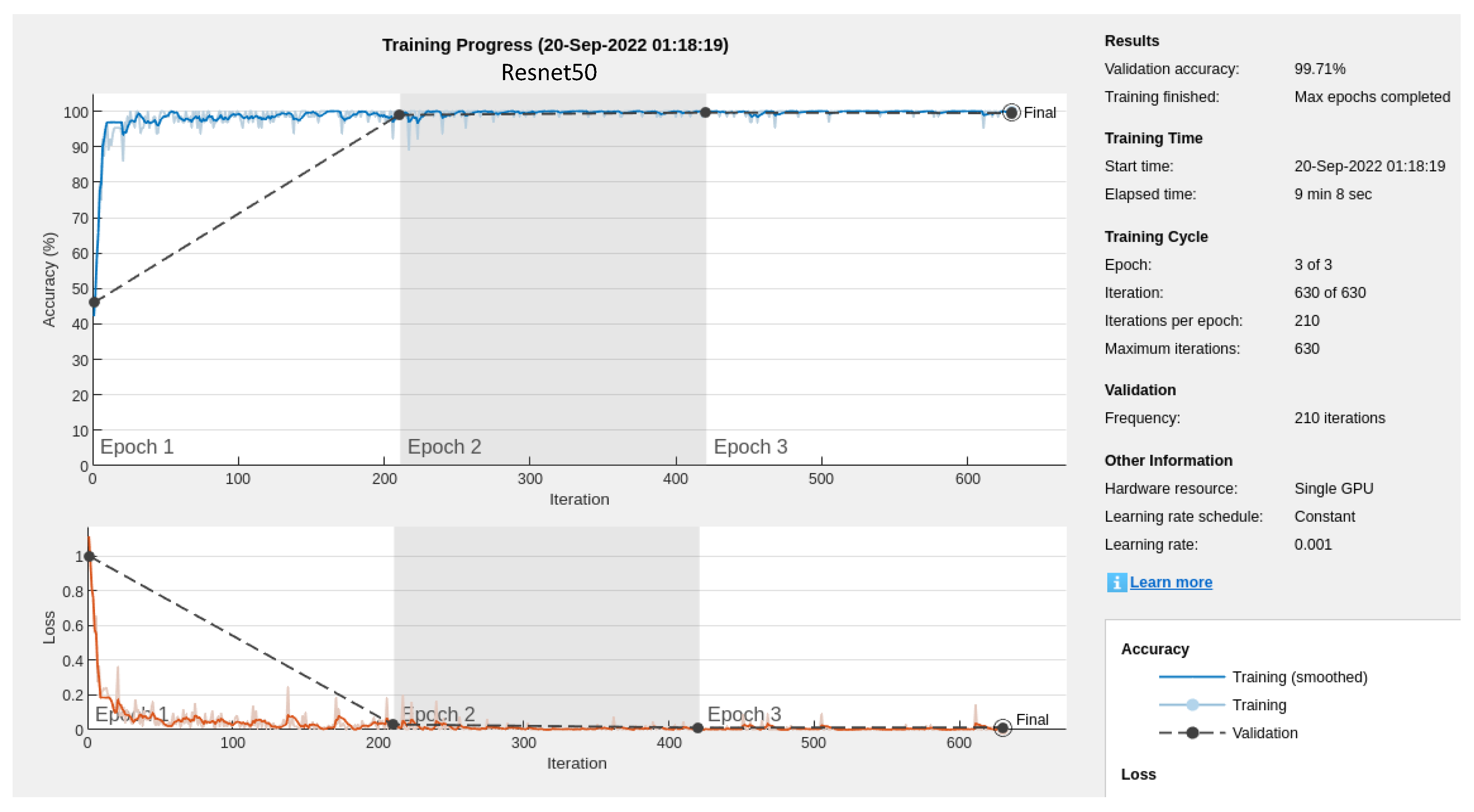
On the other hand, the training progress of the transfer learning experiments, conducted on the pre-trained networks GoogLeNet and ResNet50, are shown in Figure 6 and Figure 7, respectively. The loss function progress is depicted as well in Figure 6 and Figure 7. It can be observed that two epochs would have been sufficient, since the third epoch barely gives a significant improvement in the accuracy obtained—that is, the third epoch indicates that the accuracy cannot be improved any further.

Analyzing all the results, we observed similar performance in both models. Accuracy in the training and test processes was over 99%, which defines both as superb deep-learning models. ResNet50 is slightly better than GoogLeNet but requires more GPU time because of the greater number of layers involved. In addition to the accuracy of the classifiers, three other indicators, precision, recall and specificity, are provided in

Table 4. Indicators that define the behavior of pre-trained deep-learning network GoogLeNet; FP/FN = false positives/false negatives; and TP/TN = true positives/negatives. These values were obtained from samples not used for training and/or validating the network.

	Precision	Recall	Specificity	F1 (Har. Mean)	MCC
Annealing	0.9968	0.9859	0.9984	0.9914	0.9871
Quenching	0.9846	1	0.9922	0.9922	0.9884
Quench. + Tem	1	0.9953	1	0.9977	0.9965
Average	0.9938	0.9938	0.9969	0.9938	0.9907

Precision = TP/(TP + FP); Recall = TP/(TP + FN); Specificity = TN/(TN + TP); F1 = Harmonic mean = 2(precision × recall)/(precision + recall); and MCC = Matthew’s correlation coefficient.

and

Table 5. Indicators that define the behavior of pre-trained deep-learning network ResNet50; FP/FN = false positives/false negatives; and TP/TN = true positives/negatives. These values were obtained from samples not used for training and/or validating the network.

	Precision	Recall	Specificity	F1 (Har. Mean)	MCC
Annealing	0.9917	1	0.9962	0.9959	0.9883
Quenching	1	0.9924	1	0.9962	0.9919
Quench. + Tem	1	1	1	1	0.9965
Average	0.9972	0.9975	0.9987	0.9973	0.9922

Precision = TP/(TP + FP); Recall = TP/(TP + FN); Specificity = TN/(TN + TP); F1 = Harmonic mean = 2(precision × recall)/(precision + recall); and MCC = Matthew’s correlation coefficient.

. Precision is used to obtain the percentage of correct predictions in every class, meaning the degree of reliability, while recall is used to represent the fraction of samples that were correctly recognized—that is, the model’s detection capability [34].

The harmonic mean of recall and precision is included as well as the average value of all indicators. Finally, Matthew’s correlation coefficient was included as an indicator of the imbalance sensitivity of the process. The classification was balanced since the same number of images per class were used to train and validate the ML classifiers and the transfer-learning networks. Logically, the values obtained for Matthew´s coefficient equal almost 1.

In order to double-check the goodness of the two DL networks selected, a new experiment was performed consisting of training and validating those networks from scratch, i.e., without the pre-trained dataset. In Figure 8 and Figure 9, the accuracies of the tests and validation data are lower than the pre-trained networks in both cases. In addition, the maximum accuracy value is reached with a significantly higher number of iterations. Finally, the results are more unstable with variations of up to 25%. Consequently, it is demonstrated that the transfer-learning approach suitably fits the classification of steel microstructure images.

In Figure 10, the confusion matrixes for GoogLeNet and ResNet50 tests are represented. As it was expected, transfer-learning approaches led to best results over classical machine-learning classification models. Choosing a pre-trained deep-learning network and adapting it to the microstructure image dataset was easy and consumed adequate GPU time. The experiments yielded excellent results in test confusion matrix 9 and, in addition, it can be stated that ResNet50 is the deep-learning network that better fits this three-class steel microstructure classification problem. If the confusion matrixes are analyzed, it can be stated that annealing is the class that presents a higher number of false positives.

This appears coherent with the complexity established by the authors as a starting point based on the significant heterogeneity degree associated with the corresponding microstructures. Although annealing micrographs are the easiest to be classified, according to the essential number of key points, their heterogeneity suggest a higher probability that the system throws more false positives. We highlight the absence of false positives and negatives related to the other two categories, i.e., quenching and quenching–tempering. The authors expected some degree of confusion between these two categories since there is some visual affinity of the involved micrographs. Thus, it can be stated that the results obtained are excellent and, particularly, better with ResNet50 transfer learning, which can be considered as a good choice in future research in the field of steel microconstituent recognition.

4. Conclusions

In this research, we explored classic and large convolutional neural network models for solving an image-classification problem of low-carbon steel microstructures to identify the corresponding heat treatment applied to them. For this, an image dataset with three categories was created: annealing, quenching and quenching-tempering. This issue has great intrinsic complexity if it is considered that microstructures present a significant degree of heterogeneity inside of each group, with the greatest being the annealing group.

Part of this difficulty is due to the fact that images were obtained by means of optical microscopy at 400× magnification, which means that it is difficult to solve certain constituents and that images may present the same constituent under different aspects—notably, the perlite. Some classic machine-learning algorithms have been fed with this set of images to generate classification models for choosing the best one. The results obtained are clearly unsatisfactory due to the low accuracy reached in training and, mainly, in testing experiments.

This result brings into question the utility of classic machine learning in a microstructure image context. However, the application of the transfer-learning techniques, GoogLeNet and ResNet50, on the problem, led to obtain great results from both, with 99% accuracy in the training and testing experiments. The results permit deeper research regarding microconstituent recognition to be performed in the future by using transfer-learning techniques.

References

1. Bulgarevich, D.S.; Tsukamoto, S.; Kasuya, T.; Demura, M.; Watanabe, M. Pattern recognition with machine learning on optical microscopy images of typical metallurgical microstructures. Sci. Rep. 2018, 8, 2078. Available online: https://www.nature.com/articles/s41598-018-20438-6 (accessed on 20 November 2022). [CrossRef] [PubMed] [Green Version]
2. Bulgarevich, D.S.; Tsukamoto, S.; Kasuya, T.; Demura, M.; Watanabe, M. Automatic steel labeling on certain microstructural constituents with image processing and machine learning tools. Sci. Technol. Adv. Mater. 2019, 20, 532–542. [Google Scholar] [CrossRef] [Green Version]
3. Müller, M.; Britz, D.; Staudt, T.; Mücklich, F. Microstructural classification of bainitic subclasses in low-carbon multi-phase steels using machine learning techniques. Metals 2021, 11, 1836. [Google Scholar] [CrossRef]
4. Kim, H.; Inoue, J.; Kasuya, T. Author Correction: Unsupervised microstructure segmentation by mimicking metallurgists’ approach to pattern recognition. Sci. Rep. 2021, 11, 8548. [Google Scholar] [CrossRef]
5. Nishiura, H.; Miyamoto, A.; Ito, A.; Harada, M.; Suzuki, S.; Fujii, K.; Morifuji, H.; Takatsuka, H. Machine-learning-based quality-level-estimation system for inspecting steel microstructures. Microscopy 2022, 71, 214–222. [Google Scholar] [CrossRef]
6. Simonyan, K.; Zisserman, A. Very deep convolutional networks for large-scale image recognition. arXiv 2014, arXiv:1409.1556. Available online: https://arxiv.org/abs/1409.1556 (accessed on 30 October 2022).
7. Maemura, T.; Terasaki, H.; Tsutsui, K.; Uto, K.; Hiramatsu, S.; Hayashi, K.; Moriguchi, K.; Morito, S. Interpretability of deep learning classification for low-carbon steel microstructures. Mater. Trans. 2020, 61, 1584–1592. [Google Scholar] [CrossRef]
8. Zhu, B.; Chen, Z.; Hu, F.; Dai, X.; Wang, L.; Zhang, Y. Feature extraction and microstructural classification of hot stamping ultra-high strength steel by machine learning. JOM 2022, 74, 3466–3477. [Google Scholar] [CrossRef]
9. Motyl, M.; Madej, Ł. Supervised pearlitic–ferritic steel microstructure segmentation by u-net convolutional neural network. Archiv. Civ. Mech. Eng. 2022, 22, 206. [Google Scholar] [CrossRef]
10. Ronneberger, O.; Fischer, P.; Brox, T. U-net: Convolutional networks for biomedical image segmentation. In Lecture Notes in Computer Science; Springer: Cham, Switzerland, 2015; Volume 9351. [Google Scholar] [CrossRef] [Green Version]
11. Breumier, S.; Ostormujof, T.M.; Frincu, B.; Gey, N.; Couturier, A.; Loukachenko, N.; Aba-perea, P.; Germain, L. Leveraging EBSD data by deep learning for bainite, ferrite and martensite segmentation. Mater. Charact. 2022, 186, 111805. [Google Scholar] [CrossRef]
12. Decost, B.L.; Lei, B.; Francis, T.; Holm, E.A. High throughput quantitative metallography for complex microstructures using deep learning: A case study in ultrahigh carbon steel. Microsc. Microanal. 2019, 25, 21–29. [Google Scholar] [CrossRef] [PubMed] [Green Version]
13. Bansal, A.; Chen, X.; Russell, B.; Gupta, A.; Ramanan, D. Pixelnet: Representation of the pixels, by the pixels, and for the pixels. arXiv 2017. [Google Scholar] [CrossRef]
14. DeCost, B.L.; Hecht, M.D.; Francis, T.; Webler, B.A.; Picard, Y.N.; Holm, E.A. UHCSDB: UltraHigh Carbon Steel Micrograph DataBase. Integr. Mater. Manuf. Innov. 2017, 6, 264. [Google Scholar] [CrossRef]
15. Wang, Z.; Adachi, Y. Property prediction and properties-to-microstructure inverse analysis of steels by a machine-learning approach. Mat. Sci. Eng. A-Struct. 2019, 744, 661–670. [Google Scholar] [CrossRef]
16. Wang, Z.; Ogawa, T.; Adachi, Y. Properties-to-microstructure-to-processing inverse analysis for steels via machine learning. ISIJ Int. 2019, 59, 1691–1694. [Google Scholar] [CrossRef] [Green Version]
17. Dhola, K.; Saradva, M. A comparative evaluation of traditional machine learning and deep learning classification techniques for sentiment analysis. In Proceedings of the 2021 11th International Conference on Cloud Computing, Data Science & Engineering (Confluence), Piscataway, NJ, USA, 28–29 January 2021; pp. 932–936. [Google Scholar]
18. Wang, P.; Fan, E.; Wang, P. Comparative analysis of image classification algorithms based on traditional machine learning and deep learning. Pattern Recognit. Lett. 2021, 141, 61–67. [Google Scholar] [CrossRef]
19. Amri, A.; Ismail, A.; Zarir, A. Comparative performance of deep learning and machine learning algorithms on imbalanced handwritten data. Int. J. Adv. Comput. Sci. Appl. 2018, 9, 258–264. [Google Scholar] [CrossRef] [Green Version]
20. Giordano, M.; Maddalena, L.; Manzo, M.; Guarracino, M.R. Adversarial attacks on graph-level embedding methods: A case study. Ann. Math. Artif. Intell. 2022, 124, 1–27. [Google Scholar]
21. DeVries, T.; Taylor, G.W. Improved regularization of convolutional neural networks with cutout. arXiv 2017, arXiv:1708.04552. [Google Scholar]
22. Yun, S.; Han, D.; Chun, S.; Oh, S.J.; Yoo, Y.; Choe, J. Cut-mix: Regularization strategy to train strong classifiers with localizable features. In Proceedings of the IEEE/CVF International Conference on Computer Vision (ICCV), Seoul, Republic of Korea, 27 October–2 November 2019; pp. 6022–6031. [Google Scholar] [CrossRef] [Green Version]
23. Taylor, L.; Nitschke, G. Improving deep learning with generic data augmentation. In Proceedings of the IEEE Symposium Series on Computational Intelligence, Bangalore, India, 18–21 November 2018; pp. 1542–1547. [Google Scholar] [CrossRef]
24. Shijie, J.; Ping, W.; Peiyi, J.; Siping, H. Research on data augmentation for image classification based on convolution neural networks. In Proceedings of the Chinese Automation Congress, Jinan, China, 20–22 October 2017; pp. 4165–4170. [Google Scholar] [CrossRef]
25. Ding, J.; Li, X.; Gudivada, V.N. Augmentation and evaluation of training data for deep learning. In Proceedings of the IEEE International Conference on Big Data, Boston, MA, USA, 11–14 December 2017; pp. 2603–2611. [Google Scholar] [CrossRef]
26. Csurka, G.; Dance, C.R.; Fan, L.; Willamowski, J.; Bray, C. Visual categorization with bags of keypoints. In Workshop on Statistical Learning in Computer Vision; Springer: Berlin/Heidelberg, Germany, 2004; pp. 1–22. [Google Scholar]
27. Nowak, E.; Jurie, F.; Triggs, B. Sampling strategies for bag-of-features image classification. In Computer Vision—ECCV Lecture Notes in Computer Science; Springer: Berlin/Heidelberg, Germany, 2006; Volume 3954, pp. 490–503. [Google Scholar] [CrossRef] [Green Version]
28. Jégou, H.; Douze, M.; Schmid, C.; Pérez, P. Aggregating local descriptors into a compact image representation. In Proceedings of the 23rd IEEE Conference on Computer Vision & Pattern Recognition, San Francisco, CA, USA, 13–18 June 2010; pp. 3304–3311. [Google Scholar] [CrossRef] [Green Version]
29. Bay, H.; Ess, A.; Tuytelaars, T.; Van Gool, L. Speeded-up robust features (surf). Comput. Vis. Image Underst. 2008, 110, 346–359. [Google Scholar] [CrossRef]
30. Szegedy, C.; Liu, W.; Jia, Y.; Sermanet, P.; Reed, S.; Anguelov, D.; Erhan, D.; Vanhoucke, V.; Rabinovich, A. Going deeper with convolutions. In Proceedings of the IEEE Conference on Computer Vision and Pattern Recognition (CVPR), Boston, MA, USA, 7–12 June 2015; pp. 1–9. [Google Scholar] [CrossRef] [Green Version]
31. He, K.; Zhang, X.; Ren, S.; Sun, J. Deep Residual Learning for Image Recognition. In Proceedings of the IEEE Conference on Computer Vision and Pattern Recognition (CVPR), Las Vegas, NV, USA, 27–30 June 2016; pp. 770–778. [Google Scholar] [CrossRef] [Green Version]
32. Deng, J.; Dong, W.; Socher, R.; Li, L.; Li, K.; Fei-Fei, L. Imagenet: A large-scale hierarchical image database. In Proceedings of the IEEE Conference on Computer Vision and Pattern Recognition, Miami, FL, USA, 20–25 June 2009; pp. 248–255. [Google Scholar] [CrossRef] [Green Version]
33. Zhao, P.; Li, C.; Rahaman, M.; Xu, H.; Yang, H.; Sun, H.; Jiang, T.; Grzegorzek, M. A comparative study of deep learning classification methods on a small environmental microorganism image dataset (emds-6): From convolutional neural networks to visual transformers. Front. Microbiol. 2022, 13. [Google Scholar] [CrossRef] [PubMed]
34. Bautista-Monsalve, F.; García-Sevilla, F.; Miguel, V.; Naranjo, J.; Manjabacas, M. A Novel Machine-Learning-Based Procedure to Determine the Surface Finish Quality of Titanium Alloy Parts Obtained by Heat Assisted Single Point Incremental Forming. Metals 2021, 11, 1287. [Google Scholar] [CrossRef]
Figure 1. Typical annealing microstructures of a C45E steel (a), a C22E steel (b) and a 34CrMo4 steel (c); globular annealing of C45E steel (d).
Applsci 13 03479 g001
Figure 2. Typical quenching microstructures of C22E steel (a), C45E steel (b), 37Cr4 steel (c) and 40niCrMo6 steel (d).
Applsci 13 03479 g002
Figure 3. Typical microstructures after quenching + tempering at 450 °C for steels C45E (a), 40niCrMo6 (b) and 37Cr4 (c); (d) corresponds to a tempering temperature of 650 °C for a C45E steel.
Applsci 13 03479 g003
Figure 4. A selection of the 10 strongest keypoints in steel samples annealing (a), quenching (b) and tempering (c). 1 is the strongest keypoint and 10 the weakest.
Applsci 13 03479 g004
Figure 5. Histograms for visual word occurrence corresponding to the images of the different heat treatments. (a) Original histogram representations. (b) Histograms sorted from the strongest to the weakest feature.
Applsci 13 03479 g005
Figure 6. Accuracy and loss of training progress in the GoogLeNet transfer learning.
Applsci 13 03479 g006
Figure 7. Accuracy and loss of training progress in the ResNet50 transfer learning.
Applsci 13 03479 g007
Figure 8. Accuracy and loss of training progress in the GoogLeNet from scratch (no transfer learning).
Applsci 13 03479 g008
Figure 9. Accuracy and loss of training progress in the ResNet50 transfer learning from scratch (no transfer learning).
Applsci 13 03479 g009
Figure 10. Confusion matrixes for the pre-trained networks, GoogLeNet (a) and ResNet50 (b) used in transfer learning tests, i.e., corresponding to samples that were not used to train and/or validate the networks.
Applsci 13 03479 g010