
Exploring Maintainability Index Variants for Software Maintainability Measurement in Object-Oriented Systems

Abstract
:1. Introduction
- RQ1
- How do different Maintainability Index variants perform when utilized for the maintainability measurement of a single object-oriented software system?
- RQ2
- How do different Maintainability Index variants perform when utilized for the maintainability measurement of an object-oriented software system in the context of other systems?
- RQ2.1
- How do different Maintainability Index variants perform when utilized for maintainability measurement between different software systems?
- RQ2.2
- How do different Maintainability Index variants perform when utilized for maintainability measurement between versions of the same software system?
2. Background
2.1. Object-Oriented Software
2.2. Maintainability Measurement in Object-Oriented Software Systems
2.3. Maintainability Index Variants
3. Related Work
4. Research Method
5. Results and Data Analysis
5.1. RQ1: Maintainability Measurement in a Software System
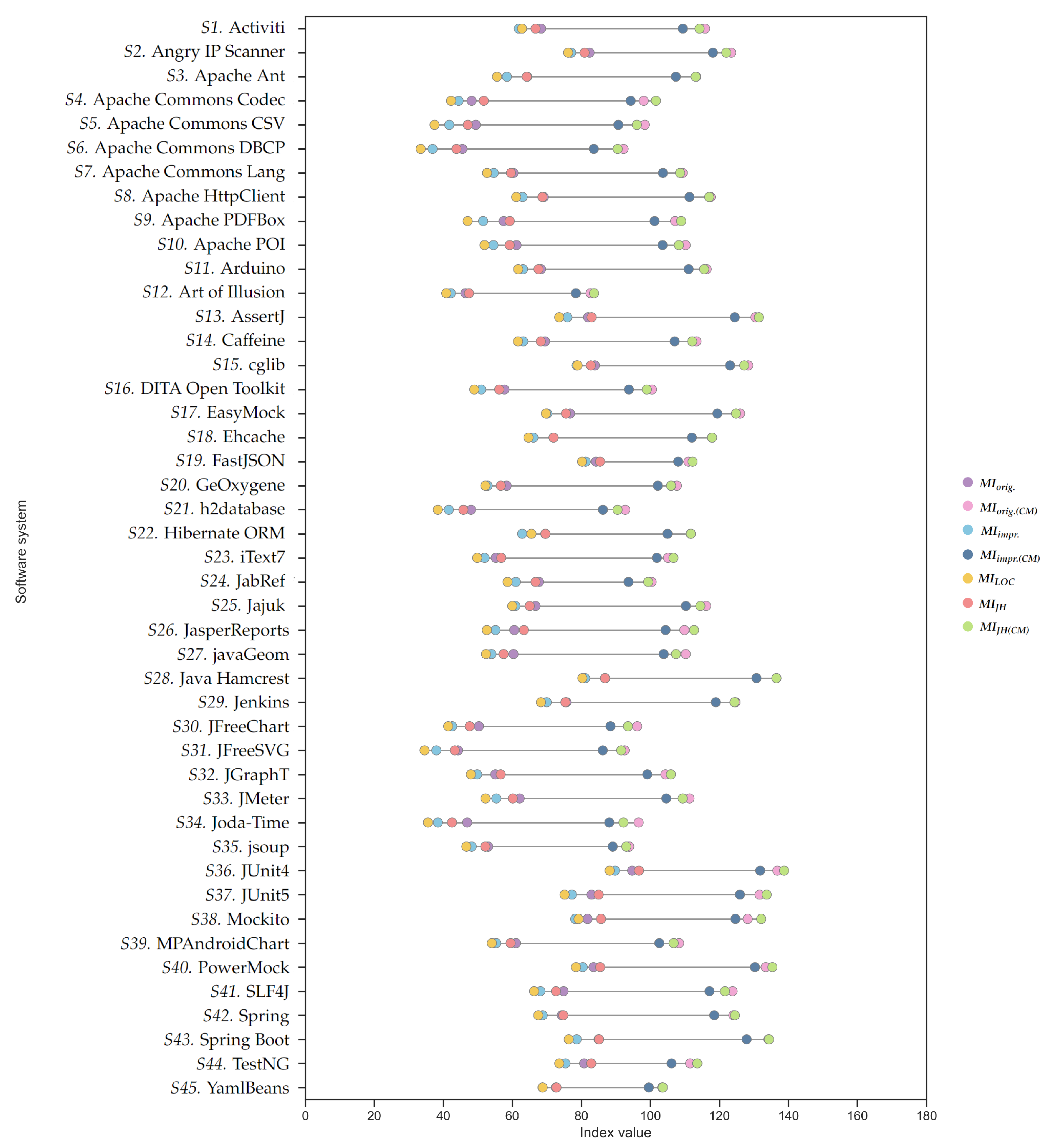
5.2. RQ2.1: Maintainability Measurement in Different Software Systems
5.3. RQ2.2: Maintainability Measurement in Versions of a Software System
6. Discussion
6.1. Summary of Research Questions and Their Answers
6.1.1. RQ1: How Do Different Maintainability Index Variants Perform When Utilized for the Maintainability Measurement of a Single Object-Oriented Software System?
6.1.2. RQ2.1: How Do Different Maintainability Index Variants Perform When Utilized for Maintainability Measurement between Different Software Systems?
6.1.3. RQ2.2: How Do Different Maintainability Index Variants Perform When Utilized for Maintainability Measurement between Versions of the Same Software System?
6.2. Theoretical and Practical Implications
6.3. Threats to Validity
6.3.1. Internal Validity
6.3.2. External Validity
7. Conclusions
Author Contributions
Funding
Institutional Review Board Statement
Informed Consent Statement
Data Availability Statement
Conflicts of Interest
Abbreviations
| Research question | |
| Original Maintainability Index | |
| Original Maintainability Index with comment part | |
| Improved Maintainability Index | |
| Improved Maintainability Index with comment part | |
| Maintainability Index using Lines Of Code only | |
| JHawk Maintainability Index | |
| JHawk Maintainability Index with comment part | |
| Visual Studio Maintainability Index | |
| Average Halstead’s Effort per module | |
| Average Halstead’s Volume per module | |
| Average Cyclomatic Complexity per module | |
| Average Lines of Code per module | |
| Average Number of Statements per module | |
| Average Percent of Lines of Comments per module | |
| S | Software system |
| Case study | |
| Average | |
| Median | |
| Standard deviation | |
| Minimum | |
| Maximum | |
| Skewness | |
| Kurtosis | |
| Confidence interval | |
| Standard error | |
| Shapiro–Wilk Test | |
| Multidimensional scaling |
Appendix A. Maintainability Index Variant Values

| Software System | MIorig. | MIorig.(CM) | MIimpr. | MIimpr.(CM) | MILOC | MIJH | MIJH(CM) |
|---|---|---|---|---|---|---|---|
| S1. Activiti | 68.36 | 115.88 | 61.90 | 109.41 | 62.82 | 66.74 | 114.26 |
| S2. Angry IP Scanner | 82.39 | 123.47 | 77.07 | 118.14 | 76.20 | 80.96 | 122.03 |
| S3. Apache Ant | 64.31 | 113.28 | 58.43 | 107.40 | 55.56 | 64.19 | 113.17 |
| S4. Apache Commons Codec | 48.21 | 98.09 | 44.44 | 94.32 | 42.26 | 51.74 | 101.63 |
| S5. Apache Commons CSV | 49.42 | 98.41 | 41.73 | 90.72 | 37.47 | 47.11 | 96.11 |
| S6. Apache Commons DBCP | 45.52 | 92.25 | 36.90 | 83.63 | 33.45 | 43.81 | 90.54 |
| S7. Apache Commons Lang | 60.33 | 109.36 | 54.63 | 103.67 | 52.68 | 59.61 | 108.64 |
| S8. Apache HttpClient | 69.14 | 117.49 | 63.00 | 111.34 | 61.14 | 68.73 | 117.07 |
| S9. Apache PDFBox | 57.51 | 107.20 | 51.55 | 101.23 | 47.06 | 59.26 | 108.95 |
| S10. Apache POI | 61.23 | 110.25 | 54.54 | 103.56 | 51.94 | 59.27 | 108.29 |
| S11. Arduino | 68.31 | 116.33 | 63.10 | 111.12 | 61.72 | 67.59 | 115.61 |
| S12. Art of Illusion | 46.44 | 82.70 | 42.19 | 78.44 | 40.87 | 47.44 | 83.70 |
| S13. AssertJ | 81.98 | 130.48 | 75.98 | 124.48 | 73.60 | 82.99 | 131.49 |
| S14. Caffeine | 69.49 | 113.37 | 63.18 | 107.06 | 61.66 | 68.26 | 112.15 |
| S15. cglib | 83.92 | 128.39 | 78.65 | 123.12 | 78.92 | 82.77 | 127.24 |
| S16. DITA Open Toolkit | 57.71 | 100.49 | 51.02 | 93.80 | 48.98 | 56.20 | 98.98 |
| S17. EasyMock | 76.74 | 126.03 | 70.14 | 119.44 | 69.75 | 75.56 | 124.85 |
| S18. Ehcache | 71.94 | 117.88 | 66.10 | 112.04 | 64.70 | 71.97 | 117.91 |
| S19. FastJSON | 84.26 | 111.06 | 81.28 | 108.08 | 80.23 | 85.44 | 112.24 |
| S20. GeOxygene | 58.36 | 107.70 | 52.84 | 102.18 | 52.19 | 56.67 | 106.01 |
| S21. h2database | 48.04 | 92.72 | 41.59 | 86.27 | 38.42 | 45.82 | 90.51 |
| S22. Hibernate ORM | 69.57 | 111.71 | 62.85 | 105.00 | 65.55 | 69.62 | 111.76 |
| S23. iText7 | 55.22 | 105.14 | 51.99 | 101.91 | 49.83 | 56.80 | 106.72 |
| S24. JabRef | 67.74 | 100.38 | 61.04 | 93.67 | 58.63 | 66.74 | 99.38 |
| S25. Jajuk | 66.73 | 116.16 | 60.89 | 110.32 | 59.98 | 65.07 | 114.50 |
| S26. JasperReports | 60.56 | 109.87 | 55.13 | 104.44 | 52.63 | 63.37 | 112.68 |
| S27. javaGeom | 60.35 | 110.29 | 53.95 | 103.89 | 52.38 | 57.50 | 107.44 |
| S28. Java Hamcrest | 86.90 | 136.57 | 81.10 | 130.77 | 80.32 | 86.87 | 136.55 |
| S29. Jenkins | 75.68 | 124.69 | 69.98 | 118.99 | 68.30 | 75.39 | 124.40 |
| S30. JFreeChart | 50.32 | 96.20 | 42.57 | 88.46 | 41.42 | 47.64 | 93.53 |
| S31. JFreeSVG | 44.29 | 92.54 | 37.98 | 86.23 | 34.56 | 43.33 | 91.58 |
| S32. JGraphT | 55.07 | 104.39 | 49.81 | 99.13 | 47.99 | 56.64 | 105.96 |
| S33. JMeter | 62.13 | 111.37 | 55.39 | 104.63 | 52.24 | 60.14 | 109.38 |
| S34. Joda-Time | 46.93 | 96.61 | 38.44 | 88.11 | 35.55 | 42.54 | 92.21 |
| S35. jsoup | 53.01 | 93.88 | 48.24 | 89.10 | 46.70 | 52.18 | 93.04 |
| S36. JUnit4 | 94.74 | 136.82 | 89.78 | 131.86 | 88.23 | 96.71 | 138.78 |
| S37. JUnit5 | 82.97 | 131.68 | 77.28 | 125.99 | 75.15 | 85.02 | 133.73 |
| S38. Mockito | 81.81 | 128.23 | 78.25 | 124.67 | 79.20 | 85.72 | 132.14 |
| S39. MPAndroidChart | 61.08 | 108.35 | 55.34 | 102.62 | 54.08 | 59.51 | 106.78 |
| S40. PowerMock | 83.55 | 133.47 | 80.41 | 130.33 | 78.47 | 85.47 | 135.39 |
| S41. SLF4J | 74.87 | 123.85 | 68.17 | 117.15 | 66.31 | 72.65 | 121.64 |
| S42. Spring | 74.35 | 124.07 | 68.81 | 118.53 | 67.54 | 74.79 | 124.51 |
| S43. Spring Boot | 85.01 | 134.27 | 78.66 | 127.92 | 76.36 | 85.13 | 134.39 |
| S44. TestNG | 80.82 | 111.54 | 75.42 | 106.15 | 73.62 | 82.89 | 113.62 |
| S45. YamlBeans | 72.62 | 103.44 | 68.75 | 99.57 | 68.80 | 72.80 | 103.63 |
| Case Study | Release | MIorig. | MIorig.(CM) | MIimpr. | MIimpr.(CM) | MILOC | MIJH | MIJH(CM) |
|---|---|---|---|---|---|---|---|---|
| CS1. AsssertJ | 1.0.0 | 85.29 | 134.60 | 78.95 | 128.26 | 75.67 | 84.71 | 134.02 |
| CS1. AsssertJ | 1.1.0 | 84.94 | 134.28 | 78.61 | 127.94 | 75.32 | 84.37 | 133.71 |
| CS1. AsssertJ | 1.2.0 | 85.10 | 134.47 | 78.75 | 128.13 | 75.49 | 84.55 | 133.92 |
| CS1. AsssertJ | 1.3.0 | 85.23 | 134.57 | 78.80 | 128.15 | 75.46 | 84.75 | 134.10 |
| CS1. AsssertJ | 1.4.0 | 85.23 | 134.16 | 78.82 | 127.75 | 75.52 | 84.78 | 133.72 |
| CS1. AsssertJ | 1.5.0 | 84.94 | 133.79 | 78.54 | 127.39 | 75.24 | 84.50 | 133.35 |
| CS1. AsssertJ | 1.6.0 | 84.90 | 133.75 | 78.48 | 127.34 | 75.22 | 84.49 | 133.34 |
| CS1. AsssertJ | 1.6.1 | 84.87 | 133.73 | 78.46 | 127.32 | 75.19 | 84.46 | 133.32 |
| CS1. AsssertJ | 1.7.0 | 84.78 | 133.68 | 78.42 | 127.32 | 75.26 | 84.45 | 133.35 |
| CS1. AsssertJ | 1.7.1 | 84.78 | 133.68 | 78.42 | 127.32 | 75.27 | 84.45 | 133.35 |
| CS1. AsssertJ | 2.0.0 | 84.09 | 133.23 | 77.96 | 127.09 | 75.00 | 84.01 | 133.14 |
| CS1. AsssertJ | 2.1.0 | 83.99 | 133.13 | 77.72 | 126.86 | 74.78 | 83.86 | 133.01 |
| CS1. AsssertJ | 2.2.0 | 84.00 | 133.36 | 77.72 | 127.09 | 74.78 | 83.89 | 133.25 |
| CS1. AsssertJ | 2.3.0 | 83.65 | 132.79 | 77.47 | 126.61 | 74.56 | 83.63 | 132.77 |
| CS1. AsssertJ | 2.4.0 | 83.00 | 132.24 | 76.84 | 126.08 | 73.94 | 83.09 | 132.33 |
| CS1. AsssertJ | 2.4.1 | 83.00 | 132.24 | 76.84 | 126.08 | 73.94 | 83.09 | 132.34 |
| CS1. AsssertJ | 2.5.0 | 82.88 | 132.10 | 76.71 | 125.93 | 73.84 | 83.05 | 132.27 |
| CS1. AsssertJ | 2.6.0 | 82.78 | 132.05 | 76.55 | 125.83 | 73.65 | 82.94 | 132.22 |
| CS1. AsssertJ | 2.7.0 | 83.35 | 132.45 | 77.23 | 126.33 | 74.39 | 83.65 | 132.74 |
| CS1. AsssertJ | 2.8.0 | 83.31 | 132.42 | 77.19 | 126.30 | 74.33 | 83.61 | 132.72 |
| CS1. AsssertJ | 2.9.0 | 83.14 | 132.28 | 77.25 | 126.39 | 74.51 | 83.76 | 132.91 |
| CS1. AsssertJ | 3.0.0 | 83.88 | 132.94 | 77.66 | 126.72 | 74.65 | 83.74 | 132.80 |
| CS1. AsssertJ | 3.1.0 | 83.64 | 132.68 | 77.35 | 126.39 | 74.35 | 83.55 | 132.58 |
| CS1. AsssertJ | 3.2.0 | 83.63 | 132.80 | 77.33 | 126.50 | 74.34 | 83.55 | 132.71 |
| CS1. AsssertJ | 3.3.0 | 83.28 | 132.10 | 77.05 | 125.87 | 74.09 | 83.26 | 132.08 |
| CS1. AsssertJ | 3.4.0 | 82.71 | 131.73 | 76.50 | 125.53 | 73.56 | 82.80 | 131.83 |
| CS1. AsssertJ | 3.4.1 | 82.71 | 131.74 | 76.51 | 125.54 | 73.56 | 82.80 | 131.83 |
| CS1. AsssertJ | 3.5.0 | 82.42 | 131.52 | 76.21 | 125.30 | 73.28 | 82.60 | 131.69 |
| CS1. AsssertJ | 3.5.1 | 82.43 | 131.52 | 76.21 | 125.31 | 73.29 | 82.60 | 131.70 |
| CS1. AsssertJ | 3.5.2 | 82.43 | 131.52 | 76.21 | 125.31 | 73.29 | 82.60 | 131.70 |
| CS1. AsssertJ | 3.6.0 | 82.32 | 131.47 | 76.06 | 125.22 | 73.16 | 82.50 | 131.66 |
| CS1. AsssertJ | 3.6.1 | 82.32 | 131.47 | 76.06 | 125.21 | 73.15 | 82.50 | 131.65 |
| CS1. AsssertJ | 3.6.2 | 82.33 | 131.48 | 76.07 | 125.23 | 73.16 | 82.51 | 131.67 |
| CS1. AsssertJ | 3.7.0 | 82.83 | 131.81 | 76.67 | 125.64 | 73.85 | 83.15 | 132.12 |
| CS1. AsssertJ | 3.8.0 | 82.87 | 131.81 | 76.70 | 125.64 | 73.87 | 83.18 | 132.12 |
| CS1. AsssertJ | 3.9.0 | 82.63 | 131.53 | 76.75 | 125.65 | 74.06 | 83.32 | 132.22 |
| CS1. AsssertJ | 3.9.1 | 81.66 | 130.73 | 75.92 | 125.00 | 73.25 | 82.60 | 131.67 |
| CS1. AsssertJ | 3.10.0 | 81.42 | 130.59 | 75.68 | 124.84 | 73.06 | 82.40 | 131.57 |
| CS1. AsssertJ | 3.11.0 | 81.24 | 130.48 | 75.38 | 124.62 | 72.89 | 82.59 | 131.83 |
| CS1. AsssertJ | 3.11.1 | 81.24 | 130.47 | 75.38 | 124.62 | 72.89 | 82.59 | 131.82 |
| CS1. AsssertJ | 3.12.0 | 81.38 | 130.55 | 75.52 | 124.69 | 73.07 | 82.66 | 131.83 |
| CS1. AsssertJ | 3.12.1 | 81.38 | 130.55 | 75.52 | 124.69 | 73.07 | 82.66 | 131.83 |
| CS1. AsssertJ | 3.12.2 | 81.40 | 130.57 | 75.53 | 124.70 | 73.08 | 82.67 | 131.84 |
| CS1. AsssertJ | 3.13.0 | 81.16 | 130.37 | 75.23 | 124.44 | 72.75 | 82.34 | 131.55 |
| CS1. AsssertJ | 3.13.1 | 81.16 | 130.37 | 75.23 | 124.44 | 72.75 | 82.34 | 131.55 |
| CS1. AsssertJ | 3.13.2 | 81.16 | 130.37 | 75.23 | 124.44 | 72.74 | 82.34 | 131.55 |
| CS1. AsssertJ | 3.14.0 | 81.35 | 130.45 | 75.43 | 124.53 | 72.95 | 82.53 | 131.63 |
| CS1. AsssertJ | 3.15.0 | 81.87 | 130.55 | 75.88 | 124.56 | 73.62 | 82.82 | 131.50 |
| CS1. AsssertJ | 3.16.0 | 81.93 | 130.71 | 75.94 | 124.73 | 73.65 | 82.92 | 131.70 |
| CS1. AsssertJ | 3.16.1 | 81.94 | 130.73 | 75.95 | 124.74 | 73.66 | 82.93 | 131.72 |
| CS1. AsssertJ | 3.17.0 | 82.26 | 130.80 | 76.24 | 124.78 | 73.87 | 83.23 | 131.76 |
| CS1. AsssertJ | 3.17.1 | 82.26 | 130.80 | 76.24 | 124.78 | 73.87 | 83.23 | 131.77 |
| CS1. AsssertJ | 3.17.2 | 82.27 | 130.82 | 76.25 | 124.80 | 73.88 | 83.24 | 131.78 |
| CS1. AsssertJ | 3.18.0 | 82.25 | 130.82 | 76.22 | 124.80 | 73.84 | 83.22 | 131.79 |
| CS1. AsssertJ | 3.18.1 | 82.15 | 130.72 | 76.18 | 124.75 | 73.80 | 83.18 | 131.75 |
| CS1. AsssertJ | 3.19.0 | 82.13 | 130.57 | 76.17 | 124.61 | 73.80 | 83.15 | 131.59 |
| CS1. AsssertJ | 3.20.0 | 82.18 | 130.66 | 76.16 | 124.63 | 73.74 | 83.15 | 131.63 |
| CS1. AsssertJ | 3.20.1 | 82.18 | 130.65 | 76.15 | 124.63 | 73.73 | 83.15 | 131.63 |
| CS1. AsssertJ | 3.20.2 | 82.17 | 130.65 | 76.14 | 124.62 | 73.73 | 83.14 | 131.62 |
| CS1. AsssertJ | 3.21.0 | 82.04 | 130.46 | 76.05 | 124.48 | 73.70 | 83.06 | 131.49 |
| CS1. AsssertJ | 3.22.0 | 81.85 | 130.36 | 75.85 | 124.36 | 73.50 | 82.88 | 131.39 |
| CS1. AsssertJ | 3.23.0 | 81.98 | 130.48 | 75.98 | 124.48 | 73.60 | 82.99 | 131.49 |
| CS1. AsssertJ | 3.23.1 | 81.98 | 130.48 | 75.98 | 124.48 | 73.60 | 82.99 | 131.49 |
| Case Study | Release | MIorig. | MIorig.(CM) | MIimpr. | MIimpr.(CM) | MILOC | MIJH | MIJH(CM) |
|---|---|---|---|---|---|---|---|---|
| CS2. Caffeine | 1.0 | 69.38 | 115.10 | 62.99 | 108.71 | 61.63 | 68.65 | 114.37 |
| CS2. Caffeine | 1.0.1 | 70.11 | 116.11 | 63.88 | 109.88 | 62.48 | 69.47 | 115.46 |
| CS2. Caffeine | 1.1.0 | 70.39 | 116.34 | 64.19 | 110.14 | 62.80 | 69.76 | 115.71 |
| CS2. Caffeine | 1.2.0 | 70.39 | 116.22 | 64.18 | 110.01 | 62.79 | 69.73 | 115.57 |
| CS2. Caffeine | 1.3.0 | 69.92 | 115.21 | 63.44 | 108.73 | 62.12 | 69.40 | 114.69 |
| CS2. Caffeine | 1.3.1 | 69.99 | 115.29 | 63.52 | 108.82 | 62.20 | 69.47 | 114.78 |
| CS2. Caffeine | 1.3.2 | 70.41 | 116.21 | 63.98 | 109.78 | 62.58 | 69.77 | 115.57 |
| CS2. Caffeine | 1.3.3 | 70.42 | 116.21 | 63.99 | 109.78 | 62.58 | 69.77 | 115.57 |
| CS2. Caffeine | 2.0.0 | 70.26 | 115.01 | 63.94 | 108.69 | 62.47 | 69.71 | 114.47 |
| CS2. Caffeine | 2.0.1 | 70.34 | 115.12 | 64.02 | 108.81 | 62.55 | 69.81 | 114.59 |
| CS2. Caffeine | 2.0.2 | 70.33 | 115.15 | 64.01 | 108.83 | 62.52 | 69.80 | 114.62 |
| CS2. Caffeine | 2.0.3 | 70.30 | 115.17 | 63.98 | 108.85 | 62.49 | 69.76 | 114.63 |
| CS2. Caffeine | 2.1.0 | 69.94 | 114.68 | 63.56 | 108.31 | 62.02 | 69.32 | 114.07 |
| CS2. Caffeine | 2.2.0 | 69.80 | 114.56 | 63.43 | 108.19 | 61.90 | 69.18 | 113.94 |
| CS2. Caffeine | 2.2.1 | 69.73 | 114.36 | 63.34 | 107.97 | 61.80 | 69.13 | 113.75 |
| CS2. Caffeine | 2.2.2 | 69.72 | 114.33 | 63.34 | 107.94 | 61.79 | 69.12 | 113.72 |
| CS2. Caffeine | 2.2.3 | 69.65 | 114.23 | 63.27 | 107.85 | 61.73 | 69.05 | 113.63 |
| CS2. Caffeine | 2.2.4 | 69.69 | 114.25 | 63.31 | 107.88 | 61.78 | 69.09 | 113.66 |
| CS2. Caffeine | 2.2.5 | 69.68 | 114.25 | 63.31 | 107.88 | 61.77 | 69.09 | 113.66 |
| CS2. Caffeine | 2.2.6 | 69.68 | 114.25 | 63.31 | 107.88 | 61.77 | 69.09 | 113.66 |
| CS2. Caffeine | 2.2.7 | 69.72 | 114.30 | 63.35 | 107.93 | 61.81 | 69.12 | 113.70 |
| CS2. Caffeine | 2.3.0 | 69.62 | 114.12 | 63.26 | 107.76 | 61.72 | 69.01 | 113.51 |
| CS2. Caffeine | 2.3.1 | 69.84 | 114.37 | 63.50 | 108.02 | 61.93 | 69.21 | 113.74 |
| CS2. Caffeine | 2.3.2 | 69.83 | 114.38 | 63.49 | 108.04 | 61.92 | 69.21 | 113.76 |
| CS2. Caffeine | 2.3.3 | 69.82 | 114.41 | 63.48 | 108.08 | 61.93 | 69.20 | 113.80 |
| CS2. Caffeine | 2.3.4 | 69.93 | 114.36 | 63.60 | 108.04 | 62.00 | 69.32 | 113.75 |
| CS2. Caffeine | 2.3.5 | 70.13 | 114.64 | 63.83 | 108.35 | 62.24 | 69.53 | 114.05 |
| CS2. Caffeine | 2.4.0 | 70.36 | 114.82 | 64.08 | 108.53 | 62.52 | 69.75 | 114.21 |
| CS2. Caffeine | 2.5.0 | 70.07 | 114.42 | 63.78 | 108.13 | 62.24 | 69.48 | 113.83 |
| CS2. Caffeine | 2.5.1 | 70.10 | 114.46 | 63.81 | 108.17 | 62.28 | 69.51 | 113.87 |
| CS2. Caffeine | 2.5.2 | 70.04 | 114.36 | 63.73 | 108.06 | 62.20 | 69.43 | 113.75 |
| CS2. Caffeine | 2.5.3 | 70.02 | 114.35 | 63.72 | 108.05 | 62.18 | 69.39 | 113.72 |
| CS2. Caffeine | 2.5.4 | 70.03 | 114.36 | 63.72 | 108.06 | 62.19 | 69.39 | 113.73 |
| CS2. Caffeine | 2.5.5 | 70.05 | 114.38 | 63.75 | 108.08 | 62.22 | 69.42 | 113.74 |
| CS2. Caffeine | 2.5.6 | 70.11 | 114.44 | 63.82 | 108.14 | 62.29 | 69.48 | 113.81 |
| CS2. Caffeine | 2.6.0 | 70.00 | 114.26 | 63.68 | 107.94 | 62.15 | 69.37 | 113.63 |
| CS2. Caffeine | 2.6.1 | 70.02 | 114.15 | 63.71 | 107.84 | 62.17 | 69.41 | 113.54 |
| CS2. Caffeine | 2.6.2 | 69.98 | 114.12 | 63.65 | 107.79 | 62.11 | 69.38 | 113.52 |
| CS2. Caffeine | 2.7.0 | 70.08 | 113.77 | 63.66 | 107.35 | 62.14 | 69.46 | 113.16 |
| CS2. Caffeine | 2.8.0 | 69.77 | 113.21 | 63.31 | 106.75 | 61.78 | 69.12 | 112.55 |
| CS2. Caffeine | 2.8.1 | 69.69 | 113.11 | 63.23 | 106.64 | 61.67 | 69.04 | 112.45 |
| CS2. Caffeine | 2.8.2 | 69.71 | 113.12 | 63.25 | 106.66 | 61.68 | 69.06 | 112.46 |
| CS2. Caffeine | 2.8.3 | 69.76 | 113.22 | 63.30 | 106.76 | 61.74 | 69.11 | 112.57 |
| CS2. Caffeine | 2.8.4 | 69.76 | 113.21 | 63.29 | 106.75 | 61.73 | 69.11 | 112.56 |
| CS2. Caffeine | 2.8.5 | 69.78 | 113.23 | 63.32 | 106.78 | 61.76 | 69.14 | 112.59 |
| CS2. Caffeine | 2.8.6 | 69.59 | 112.94 | 63.08 | 106.43 | 61.49 | 68.87 | 112.22 |
| CS2. Caffeine | 2.8.7 | 69.42 | 112.64 | 62.90 | 106.12 | 61.31 | 68.68 | 111.91 |
| CS2. Caffeine | 2.8.8 | 69.42 | 112.64 | 62.90 | 106.12 | 61.30 | 68.68 | 111.91 |
| CS2. Caffeine | 2.9.0 | 69.35 | 112.62 | 62.83 | 106.10 | 61.24 | 68.67 | 111.94 |
| CS2. Caffeine | 2.9.1 | 69.28 | 112.52 | 62.76 | 105.99 | 61.17 | 68.59 | 111.82 |
| CS2. Caffeine | 2.9.2 | 69.18 | 112.37 | 62.64 | 105.82 | 61.05 | 68.46 | 111.65 |
| CS2. Caffeine | 2.9.3 | 69.02 | 112.11 | 62.45 | 105.55 | 60.87 | 68.29 | 111.39 |
| CS2. Caffeine | 3.0.0 | 69.70 | 112.56 | 63.28 | 106.13 | 61.77 | 68.94 | 111.79 |
| CS2. Caffeine | 3.0.1 | 69.69 | 112.53 | 63.27 | 106.11 | 61.75 | 68.93 | 111.77 |
| CS2. Caffeine | 3.0.2 | 69.66 | 112.91 | 63.23 | 106.48 | 61.71 | 68.85 | 112.10 |
| CS2. Caffeine | 3.0.3 | 70.34 | 114.05 | 63.97 | 107.68 | 62.42 | 69.43 | 113.14 |
| CS2. Caffeine | 3.0.4 | 71.32 | 115.60 | 65.16 | 109.44 | 63.50 | 70.45 | 114.74 |
| CS2. Caffeine | 3.0.5 | 71.30 | 115.51 | 65.14 | 109.35 | 63.48 | 70.44 | 114.64 |
| CS2. Caffeine | 3.0.6 | 69.75 | 113.75 | 63.36 | 107.37 | 61.80 | 68.47 | 112.47 |
| CS2. Caffeine | 3.1.0 | 69.37 | 113.26 | 63.06 | 106.95 | 61.50 | 68.22 | 112.11 |
| CS2. Caffeine | 3.1.1 | 69.49 | 113.37 | 63.18 | 107.06 | 61.66 | 68.26 | 112.15 |
| Case Study | Release | MIorig. | MIorig.(CM) | MIimpr. | MIimpr.(CM) | MILOC | MIJH | MIJH(CM) |
|---|---|---|---|---|---|---|---|---|
| CS3. Joda-Time | 0.9 | 59.04 | 104.72 | 52.37 | 98.05 | 50.51 | 57.43 | 103.12 |
| CS3. Joda-Time | 0.9.5 | 58.99 | 101.47 | 51.45 | 93.93 | 50.84 | 56.77 | 99.25 |
| CS3. Joda-Time | 1.0 | 54.77 | 104.65 | 46.70 | 96.57 | 44.74 | 50.68 | 100.55 |
| CS3. Joda-Time | 1.1 | 53.45 | 103.29 | 45.37 | 95.22 | 43.20 | 49.43 | 99.28 |
| CS3. Joda-Time | 1.2 | 55.59 | 105.39 | 47.81 | 97.61 | 45.61 | 51.77 | 101.57 |
| CS3. Joda-Time | 1.2.1 | 52.22 | 102.02 | 44.12 | 93.92 | 41.92 | 48.04 | 97.84 |
| CS3. Joda-Time | 1.3 | 53.49 | 103.30 | 45.52 | 95.33 | 43.15 | 49.37 | 99.18 |
| CS3. Joda-Time | 1.4 | 52.98 | 102.84 | 44.94 | 94.80 | 42.53 | 48.79 | 98.65 |
| CS3. Joda-Time | 1.5 | 52.68 | 102.51 | 44.64 | 94.47 | 42.17 | 48.53 | 98.36 |
| CS3. Joda-Time | 1.5.1 | 52.67 | 102.50 | 44.63 | 94.46 | 42.16 | 48.52 | 98.35 |
| CS3. Joda-Time | 1.5.2 | 52.64 | 102.47 | 44.61 | 94.44 | 42.13 | 48.50 | 98.33 |
| CS3. Joda-Time | 1.6.0 | 52.38 | 102.20 | 44.34 | 94.16 | 41.84 | 48.23 | 98.05 |
| CS3. Joda-Time | 1.6.1 | 52.34 | 102.16 | 44.30 | 94.12 | 41.80 | 48.19 | 98.00 |
| CS3. Joda-Time | 1.6.2 | 52.34 | 102.16 | 44.30 | 94.12 | 41.80 | 48.18 | 98.00 |
| CS3. Joda-Time | 2.0 | 47.75 | 97.60 | 39.28 | 89.13 | 36.60 | 43.09 | 92.94 |
| CS3. Joda-Time | 2.1 | 47.67 | 97.52 | 39.21 | 89.05 | 36.52 | 43.01 | 92.85 |
| CS3. Joda-Time | 2.2 | 47.52 | 97.36 | 39.04 | 88.88 | 36.34 | 42.84 | 92.67 |
| CS3. Joda-Time | 2.3 | 47.49 | 97.31 | 39.00 | 88.83 | 36.31 | 42.82 | 92.64 |
| CS3. Joda-Time | 2.4 | 47.60 | 97.41 | 39.13 | 88.94 | 36.44 | 42.93 | 92.74 |
| CS3. Joda-Time | 2.5 | 47.51 | 97.31 | 39.04 | 88.83 | 36.37 | 42.84 | 92.64 |
| CS3. Joda-Time | 2.6 | 47.53 | 97.32 | 39.05 | 88.84 | 36.38 | 42.85 | 92.65 |
| CS3. Joda-Time | 2.7 | 47.53 | 97.33 | 39.06 | 88.85 | 36.39 | 42.86 | 92.65 |
| CS3. Joda-Time | 2.8 | 47.53 | 97.32 | 39.06 | 88.85 | 36.39 | 42.86 | 92.65 |
| CS3. Joda-Time | 2.8.1 | 47.53 | 97.32 | 39.06 | 88.85 | 36.39 | 42.86 | 92.65 |
| CS3. Joda-Time | 2.8.2 | 47.53 | 97.32 | 39.06 | 88.85 | 36.39 | 42.86 | 92.65 |
| CS3. Joda-Time | 2.9 | 47.43 | 97.21 | 38.95 | 88.73 | 36.28 | 42.75 | 92.53 |
| CS3. Joda-Time | 2.9.1 | 47.42 | 97.21 | 38.94 | 88.73 | 36.28 | 42.74 | 92.52 |
| CS3. Joda-Time | 2.9.2 | 47.40 | 97.19 | 38.93 | 88.71 | 36.25 | 42.72 | 92.50 |
| CS3. Joda-Time | 2.9.3 | 47.40 | 97.18 | 38.92 | 88.70 | 36.25 | 42.72 | 92.50 |
| CS3. Joda-Time | 2.9.4 | 47.48 | 97.26 | 39.01 | 88.79 | 36.34 | 42.81 | 92.59 |
| CS3. Joda-Time | 2.9.5 | 47.42 | 97.19 | 38.94 | 88.71 | 36.27 | 42.74 | 92.51 |
| CS3. Joda-Time | 2.9.6 | 47.41 | 97.18 | 38.93 | 88.70 | 36.26 | 42.73 | 92.50 |
| CS3. Joda-Time | 2.9.7 | 47.41 | 97.18 | 38.93 | 88.70 | 36.26 | 42.73 | 92.51 |
| CS3. Joda-Time | 2.9.8 | 47.43 | 97.21 | 38.96 | 88.73 | 36.29 | 42.76 | 92.53 |
| CS3. Joda-Time | 2.9.9 | 47.43 | 97.21 | 38.96 | 88.73 | 36.29 | 42.76 | 92.53 |
| CS3. Joda-Time | 2.10 | 47.41 | 97.18 | 38.93 | 88.70 | 36.27 | 42.74 | 92.51 |
| CS3. Joda-Time | 2.10.1 | 47.40 | 97.17 | 38.92 | 88.69 | 36.25 | 42.72 | 92.49 |
| CS3. Joda-Time | 2.10.2 | 47.39 | 97.16 | 38.91 | 88.68 | 36.24 | 42.72 | 92.48 |
| CS3. Joda-Time | 2.10.3 | 47.36 | 97.12 | 38.89 | 88.65 | 36.22 | 42.69 | 92.45 |
| CS3. Joda-Time | 2.10.4 | 47.36 | 97.12 | 38.89 | 88.65 | 36.22 | 42.69 | 92.45 |
| CS3. Joda-Time | 2.10.5 | 47.36 | 97.12 | 38.89 | 88.65 | 36.22 | 42.69 | 92.45 |
| CS3. Joda-Time | 2.10.6 | 47.36 | 97.12 | 38.89 | 88.65 | 36.22 | 42.69 | 92.45 |
| CS3. Joda-Time | 2.10.7 | 47.28 | 97.03 | 38.80 | 88.55 | 36.13 | 42.59 | 92.34 |
| CS3. Joda-Time | 2.10.8 | 47.28 | 97.03 | 38.80 | 88.55 | 36.13 | 42.59 | 92.34 |
| CS3. Joda-Time | 2.10.9 | 47.28 | 97.03 | 38.80 | 88.55 | 36.13 | 42.59 | 92.34 |
| CS3. Joda-Time | 2.10.10 | 47.28 | 97.03 | 38.80 | 88.55 | 36.13 | 42.59 | 92.34 |
| CS3. Joda-Time | 2.10.11 | 47.27 | 97.02 | 38.79 | 88.54 | 36.12 | 42.59 | 92.34 |
| CS3. Joda-Time | 2.10.12 | 47.27 | 97.02 | 38.79 | 88.54 | 36.12 | 42.59 | 92.34 |
| CS3. Joda-Time | 2.10.13 | 47.27 | 97.02 | 38.79 | 88.54 | 36.12 | 42.59 | 92.34 |
| CS3. Joda-Time | 2.10.14 | 47.27 | 97.02 | 38.79 | 88.54 | 36.12 | 42.59 | 92.34 |
| CS3. Joda-Time | 2.11.0 | 46.93 | 96.61 | 38.44 | 88.11 | 35.55 | 42.54 | 92.21 |
| CS3. Joda-Time | 2.11.1 | 46.93 | 96.61 | 38.44 | 88.11 | 35.55 | 42.54 | 92.21 |
References
- ISO/IEC/IEEE 14764:2022; Software engineering—Software Life Cycle Processes—Maintenance. International Organization for Standardization: Geneva, Switzerland, 2022.
- Christa, S.; Madhusudhan, V.; Suma, V.; Rao, J.J. Software Maintenance: From the Perspective of Effort and Cost Requirement. In Proceedings of the International Conference on Data Engineering and Communication Technology, Maharashtra, India, 10–11 March 2017; Satapathy, S., Bhateja, V., Joshi, A., Eds.; Springer: Singapore, 2017; pp. 759–768. [Google Scholar]
- Granja-Alvarez, J.C.; Barranco-García, M.J. A Method for Estimating Maintenance Cost in a Software Project: A Case Study. J. Softw. Maint. 1997, 9, 161–175. [Google Scholar] [CrossRef]
- Ren, Y.; Xing, T.; Chen, X.; Chai, X. Research on Software Maintenance Cost of Influence Factor Analysis and Estimation Method. In Proceedings of the 2011 3rd International Workshop on Intelligent Systems and Applications, Wuhan, China, 28–29 May 2011; pp. 1–4. [Google Scholar] [CrossRef]
- ISO/IEC 25010:2011; Systems and Software Engineering—Systems and Software Quality Requirements and Evaluation (SQuaRE)—System and Software Quality Models. International Organization for Standardization: Geneva, Switzerland, 2017.
- Alsolai, H.; Roper, M. A systematic literature review of machine learning techniques for software maintainability prediction. Inf. Softw. Technol. 2020, 119, 106214. [Google Scholar] [CrossRef]
- Riaz, M.; Mendes, E.; Tempero, E. A systematic review of software maintainability prediction and metrics. In Proceedings of the 2009 3rd International Symposium on Empirical Software Engineering and Measurement, Lake Buena Vista, FL, USA, 15–16 October 2009; pp. 367–377. [Google Scholar] [CrossRef]
- Oman, P.; Hagemeister, J. Construction and testing of polynomials predicting software maintainability. Oregon Workshop on Software Metrics. J. Syst. Softw. 1994, 24, 251–266. [Google Scholar] [CrossRef]
- Coleman, D.; Ash, D.; Lowther, B.; Oman, P. Using metrics to evaluate software system maintainability. Computer 1994, 27, 44–49. [Google Scholar] [CrossRef]
- Welker, K.D.; Oman, P.W.; Atkinson, G.G. Development and Application of an Automated Source Code Maintainability Index. J. Softw. Maint. 1997, 9, 127–159. [Google Scholar] [CrossRef]
- Najm, N. Measuring Maintainability Index of a Software Depending on Line of Code Only. IOSR J. Comput. Eng. 2014, 16, 64–69. [Google Scholar] [CrossRef]
- Microsoft. Visual Studio. 2021. Available online: https://visualstudio.microsoft.com/ (accessed on 20 December 2021).
- Virtual Machinery. MI and MINC—Maintainability Index. 2021. Available online: http://www.virtualmachinery.com/sidebar4.htm (accessed on 20 December 2021).
- Kaur, K.; Singh, H. Determination of Maintainability Index for Object Oriented Systems. Determ. Maintainab. Index Object Oriented Syst. 2011, 36, 1–6. [Google Scholar] [CrossRef]
- Kaur, A.; Kaur, K.; Pathak, K. A proposed new model for maintainability index of open source software. In Proceedings of the 3rd International Conference on Reliability, Infocom Technologies and Optimization, Noida, India, 8–10 October 2014; pp. 1–6. [Google Scholar] [CrossRef]
- Misra, S.C. Modeling Design/Coding Factors That Drive Maintainability of Software Systems. Softw. Qual. J. 2005, 13, 297–320. [Google Scholar] [CrossRef]
- Madhwaraj, K.G. Empirical comparison of two metrics suites for maintainability prediction in packages of object-oriented systems: A case study of open source software. J. Comput. Sci. 2014, 10, 2330–2338. [Google Scholar] [CrossRef] [Green Version]
- Welker, K.D. The software maintainability index revisited. CrossTalk 2001, 14, 18–21. [Google Scholar]
- Sjøberg, D.I.K.; Anda, B.; Mockus, A. Questioning software maintenance metrics: A comparative case study. In Proceedings of the 2012 ACM-IEEE International Symposium on Empirical Software Engineering and Measurement, Lund, Sweden, 19–20 September 2012; pp. 107–110. [Google Scholar] [CrossRef]
- Counsell, S.; Liu, X.; Eldh, S.; Tonelli, R.; Marchesi, M.; Concas, G.; Murgia, A. Re-visiting the ‘Maintainability Index’ Metric from an Object-Oriented Perspective. In Proceedings of the 2015 41st Euromicro Conference on Software Engineering and Advanced Applications, Madeira, Portugal, 26–28 August 2015; pp. 84–87. [Google Scholar] [CrossRef]
- Seref, B.; Tanriover, O. Software code maintainability: A literature review. Int. J. Softw. Eng. Appl. 2016, 7, 3. [Google Scholar] [CrossRef]
- Ganpati, A.; Kalia, A.; Singh, H. A comparative study of maintainability index of open source software. Int. J. Emerg. Technol. Adv. Eng. 2012, 2, 228–230. [Google Scholar]
- Fedoseev, K.; Askarbekuly, N.; Uzbekova, E.; Mazzara, M. Application of Data-Oriented Design in Game Development. J. Phys. Conf. Ser. 2020, 1694, 106218. [Google Scholar] [CrossRef]
- Molnar, A.; Motogna, S. Discovering Maintainability Changes in Large Software Systems. In Proceedings of the 27th International Workshop on Software Measurement and 12th International Conference on Software Process and Product Measurement, Gothenburg, Sweden, 25–27 October 2017; Association for Computing Machinery: New York, NY, USA, 2017; pp. 88–93. [Google Scholar] [CrossRef]
- Papamichail, M.D.; Symeonidis, A.L. A generic methodology for early identification of non-maintainable source code components through analysis of software releases. Inf. Softw. Technol. 2020, 118, 106218. [Google Scholar] [CrossRef]
- Kencana, G.H.; Saleh, A.; Darwito, H.A.; Rachmadi, R.R.; Sari, E.M. Comparison of Maintainability Index Measurement from Microsoft CodeLens and Line of Code. In Proceedings of the 2020 7th International Conference on Electrical Engineering, Computer Sciences and Informatics (EECSI), Yogyakarta, Indonesia, 1–2 October 2020; pp. 235–239. [Google Scholar]
- Şanlıalp, İ.; Öztürk, M.M.; Yiğit, T. Energy Efficiency Analysis of Code Refactoring Techniques for Green and Sustainable Software in Portable Devices. Electronics 2022, 11, 442. [Google Scholar] [CrossRef]
- Zhou, Y.; Xu, B. Predicting the maintainability of open source software using design metrics. Wuhan Univ. J. Nat. Sci. 2008, 13, 14–20. [Google Scholar] [CrossRef]
- Chowdhury, S.; Holmes, R.; Zaidman, A.; Kazman, R. Revisiting the debate: Are code metrics useful for measuring maintenance effort? Empir. Softw. Eng. 2022, 27, 1–31. [Google Scholar] [CrossRef]
- Strečanský, P.; Chren, S.; Rossi, B. Comparing Maintainability Index, SIG Method, and SQALE for Technical Debt Identification. In Proceedings of the 35th Annual ACM Symposium on Applied Computing, Brno, Czech Republic, 30 March–3 April 2020; Association for Computing Machinery: New York, NY, USA, 2020; pp. 121–124. [Google Scholar] [CrossRef] [Green Version]
- Arisholm, E.; Briand, L.C.; Johannessen, E.B. A systematic and comprehensive investigation of methods to build and evaluate fault prediction models. J. Syst. Softw. 2010, 83, 2–17. [Google Scholar] [CrossRef]
- Mauša, G.; Galinac Grbac, T. Co-evolutionary multi-population genetic programming for classification in software defect prediction: An empirical case study. Appl. Soft Comput. 2017, 55, 331–351. [Google Scholar] [CrossRef]
- Gradišnik, M.; Beranič, T.; Karakatič, S. Impact of historical software metric changes in predicting future maintainability trends in open-source software development. Appl. Sci. 2020, 10, 4624. [Google Scholar] [CrossRef]
- Kaur, L.; Mishra, A. A comparative analysis of evolutionary algorithms for the prediction of software change. In Proceedings of the 2018 International Conference on Innovations in Information Technology (IIT), Al Ain, United Arab Emirates, 18–19 November 2018; pp. 187–192. [Google Scholar] [CrossRef]
- Reddy, B.R.; Ojha, A. Performance of maintainability index prediction models: A feature selection based study. Evol. Syst. 2019, 10, 179–204. [Google Scholar] [CrossRef]
- Bray, M.; Brune, K.; Fisher, D.A.; Foreman, J.; Gerken, M. C4 Software Technology Reference Guide-A Prototype; Technical Report; Software Engineering Institute—Carnegie Mellon University: Pittsburgh, PA, USA, 1997. [Google Scholar]
- GitHub. The 2021 State of the Octoverse. 2021. Available online: https://octoverse.github.com/ (accessed on 20 December 2021).
- Stack Overflow. Stack Overflow Developer Survey. 2021. Available online: https://insights.stackoverflow.com/survey/2021 (accessed on 20 December 2021).
- Puntigam, F. Interfaces of Active Objects with Internal Concurrency. In Proceedings of the 1st International Workshop on Distributed Objects for the 21st Century, Genova, Italy, 6–10 July 2009; Association for Computing Machinery: New York, NY, USA, 2009. [Google Scholar] [CrossRef]
- Murthy, A.R.C.; Palani, G.; Iyer, N.R. Object-oriented programming paradigm for damage tolerant evaluation of engineering structural components. Adv. Eng. Softw. 2011, 42, 12–24. [Google Scholar] [CrossRef]
- Brito e Abreu, F.; Melo, W. Evaluating the impact of object-oriented design on software quality. In Proceedings of the 3rd International Software Metrics Symposium, Berlin, Germany, 25–26 March 1996; pp. 90–99. [Google Scholar] [CrossRef] [Green Version]
- Coleman, D. Assessing maintainability. In Proceedings of the Software Engineering Productivity Conference, Salt Lake City, UT, USA, 7 April 1992; pp. 525–532. [Google Scholar]
- Elmidaoui, S.; Cheikhi, L.; Idri, A.; Abran, A. Empirical studies on software product maintainability prediction: A systematic mapping and review. E-Inform. Softw. Eng. J. 2019, 13, 141–202. [Google Scholar]
- Zighed, N.; Bounour, N.; Seriai, A.D. Comparative Analysis of Object-Oriented Software Maintainability Prediction Models. Found. Comput. Decis. Sci. 2018, 43, 359–374. [Google Scholar] [CrossRef] [Green Version]
- Ardito, L.; Coppola, R.; Barbato, L.; Verga, D. A tool-based perspective on software code maintainability metrics: A systematic literature review. Sci. Program. 2020, 2020, 8840389. [Google Scholar] [CrossRef]
- Virtual Machinery. JHawk. 2021. Available online: http://www.virtualmachinery.com/jhawkprod.htm (accessed on 20 December 2021).
- Lacchia, M. Radon. 2021. Available online: https://radon.readthedocs.io/ (accessed on 20 December 2021).
- Verifysoft Technology. Testwell CMT++/CMTJava. 2021. Available online: https://www.verifysoft.com/en_cmtx.html (accessed on 20 December 2021).
- Li, W.; Henry, S. Object-oriented metrics that predict maintainability. Object-Oriented Software. J. Syst. Softw. 1993, 23, 111–122. [Google Scholar] [CrossRef]
- Malhotra, R.; Khanna, M. Particle swarm optimization-based ensemble learning for software change prediction. Inf. Softw. Technol. 2018, 102, 65–84. [Google Scholar] [CrossRef]
- Elish, M.O.; Aljamaan, H.; Ahmad, I. Three empirical studies on predicting software maintainability using ensemble methods. Soft Comput. 2015, 19, 2511–2524. [Google Scholar] [CrossRef]
- Bandi, R.; Vaishnavi, V.; Turk, D. Predicting maintenance performance using object-oriented design complexity metrics. IEEE Trans. Softw. Eng. 2003, 29, 77–87. [Google Scholar] [CrossRef]
- Fioravanti, F.; Nesi, P. Estimation and prediction metrics for adaptive maintenance effort of object-oriented systems. IEEE Trans. Softw. Eng. 2001, 27, 1062–1084. [Google Scholar] [CrossRef]
- Hayes, J.; Patel, S.; Zhao, L. A metrics-based software maintenance effort model. In Proceedings of the 8th European Conference on Software Maintenance and Reengineering, Tampere, Finland, 24–26 March 2004; pp. 254–258. [Google Scholar] [CrossRef]
- De Lucia, A.; Pompella, E.; Stefanucci, S. Assessing effort estimation models for corrective maintenance through empirical studies. Inf. Softw. Technol. 2005, 47, 3–15. [Google Scholar] [CrossRef]
- Dahiya, S.S.; Chhabra, J.K.; Kumar, S. Use of genetic algorithm for software maintainability metrics’ conditioning. In Proceedings of the 15th International Conference on Advanced Computing and Communications (ADCOM 2007), Guwahati, India, 18–21 December 2007; pp. 87–92. [Google Scholar] [CrossRef]
- Sharma, A.; Grover, P.; Kumar, R. Predicting maintainability of component-based systems by using fuzzy logic. In Proceedings of the International Conference on Contemporary Computing, Noida, India, 17–19 August 2009; Springer: Berlin/Heidelberg, Germany, 2009; pp. 581–591. [Google Scholar]
- Dubey, S.K.; Rana, A. A fuzzy approach for evaluation of maintainability of object oriented software system. Int. J. Comput. Appl. 2012, 49, 1–6. [Google Scholar]
- Pratap, A.; Chaudhary, R.; Yadav, K. Estimation of software maintainability using fuzzy logic technique. In Proceedings of the 2014 International Conference on Issues and Challenges in Intelligent Computing Techniques (ICICT), Ghaziabad, India, 7–8 February 2014; pp. 486–492. [Google Scholar] [CrossRef]
- Revilla, M.A. Correlations between Internal Software Metrics and Software Dependability in a Large Population of Small C/C++ Programs. In Proceedings of the 18th IEEE International Symposium on Software Reliability (ISSRE ’07), Trollhattan, Sweden, 5–9 November 2007; pp. 203–208. [Google Scholar] [CrossRef]
- Microsoft. Visual Studio—Maintainability Index. 2021. Available online: https://docs.microsoft.com/en-us/visualstudio/code-quality/code-metrics-maintainability-index-range-and-meaning (accessed on 20 December 2021).
- Molnar, A.J.; Motogna, S. A Study of Maintainability in Evolving Open-Source Software. In Proceedings of the Evaluation of Novel Approaches to Software Engineering: 15th International Conference, ENASE 2020, Prague, Czech Republic, 5–6 May 2020; Revised Selected Papers 15. Springer: Berlin/Heidelberg, Germany, 2021; pp. 261–282. [Google Scholar]
- Chowdhury, S.A.; Uddin, G.; Holmes, R. An Empirical Study on Maintainable Method Size in Java. In Proceedings of the 19th International Conference on Mining Software Repositories, Pittsburgh, PA, USA, 23–24 May 2022; Association for Computing Machinery: New York, NY, USA, 2022; pp. 252–264. [Google Scholar] [CrossRef]
- Prabowo, G.; Suryotrisongko, H.; Tjahyanto, A. A Tale of Two Development Approach: Empirical Study on The Maintainability and Modularity of Android Mobile Application with Anti-Pattern and Model-View-Presenter Design Pattern. In Proceedings of the 2018 International Conference on Electrical Engineering and Informatics (ICELTICs), Banda Aceh, Indonesia, 19–20 September 2018; pp. 149–154. [Google Scholar] [CrossRef]
- Singh, N.; Singh, D.P.; Pant, B.; Tiwari, U.K. μBIGMSA-Microservice-Based Model for Big Data Knowledge Discovery: Thinking Beyond the Monoliths. Wirel. Pers. Commun. 2021, 116, 2819–2833. [Google Scholar] [CrossRef]
- Wilson, A.; Wedyan, F.; Omari, S. An Empirical Evaluation and Comparison of the Impact of MVVM and MVC GUI Driven Application Architectures on Maintainability and Testability. In Proceedings of the 2022 International Conference on Intelligent Data Science Technologies and Applications (IDSTA), San Antonio, TX, USA, 5–7 September 2022; pp. 101–108. [Google Scholar] [CrossRef]
- De Stefano, M.; Iannone, E.; Pecorelli, F.; Tamburri, D.A. Impacts of software community patterns on process and product: An empirical study. Sci. Comput. Program. 2022, 214, 102731. [Google Scholar] [CrossRef]
- Lavazza, L.; Abualkishik, A.Z.; Liu, G.; Morasca, S. An empirical evaluation of the “Cognitive Complexity” measure as a predictor of code understandability. J. Syst. Softw. 2023, 197, 111561. [Google Scholar] [CrossRef]
- Cohen, J. Statistical Power Analysis for the Behavioral Sciences; Routledge Academic: Milton Park, UK, 1988. [Google Scholar]
- Sawilowsky, S.S. New effect size rules of thumb. J. Mod. Appl. Stat. Methods 2009, 8, 26. [Google Scholar] [CrossRef]
- Kerby, D.S. The simple difference formula: An approach to teaching nonparametric correlation. Compr. Psychol. 2014, 3, 11-IT. [Google Scholar] [CrossRef]
- Schober, P.; Boer, C.; Schwarte, L.A. Correlation coefficients: Appropriate use and interpretation. Anesth. Analg. 2018, 126, 1763–1768. [Google Scholar] [CrossRef]
- Hout, M.C.; Papesh, M.H.; Goldinger, S.D. Multidimensional scaling. Wiley Interdiscip. Rev. Cogn. Sci. 2013, 4, 93–103. [Google Scholar] [CrossRef]
- Vijaya; Sharma, S.; Batra, N. Comparative Study of Single Linkage, Complete Linkage, and Ward Method of Agglomerative Clustering. In Proceedings of the 2019 International Conference on Machine Learning, Big Data, Cloud and Parallel Computing (COMITCon), Faridabad, India, 14–16 February 2019; pp. 568–573. [Google Scholar] [CrossRef]
- Heričko, T.; Šumak, B. Analyzing Linter Usage and Warnings Through Mining Software Repositories: A Longitudinal Case Study of JavaScript Packages. In Proceedings of the 2022 45th Jubilee International Convention on Information, Communication and Electronic Technology (MIPRO), Opatija, Croatia, 23–27 May 2022; pp. 1375–1380. [Google Scholar] [CrossRef]


| Computational Complexity | Logical Complexity | Software Size | Code Documentation | |||
|---|---|---|---|---|---|---|
| Maintainability Index Variant | Halstead’s Effort | Halstead’s Volume | McCabe’s Cyclomatic Complexity | Lines of Code | Number of Statements | Percent of Lines of Comments |
| X | X | X | ||||
| X | X | X | X | |||
| X | X | X | ||||
| X | X | X | X | |||
| X | ||||||
| X | X | X | ||||
| X | X | X | X | |||
| X | X | X | ||||
| Maintainability Index Variant | Example Study Using the Variant | Programming Language of Object-Oriented Software Systems Used in the Study |
|---|---|---|
| [10] | C++ | |
| [34,64] | Java | |
| [10] | C++ | |
| [14,20] | Java | |
| [27] | C# | |
| [22] | C++ | |
| [15,27,29,33,63,67,68] | Java | |
| [67] | Python | |
| [16] | C++ | |
| [28] | Java | |
| [65] | Python | |
| [26] | C# | |
| [31,32,62] | Java | |
| [31,32] | Java | |
| [23,26,66] | C# | |
| [24,25,35] | Java | |
| [30] | Python |
| Study | Compared Software Measures | Comparison Objective | Subject Software Systems | Research Findings |
|---|---|---|---|---|
| Kaur and Singh [14] | Maintainability Index (), proposed maintainability metric | Validating a new measure | Releases of three Java software systems | N/A |
| Kaur et al. [15] | Maintainability Index (), change metric | Evaluating the maintainability prediction power of the Index for object-oriented software on the class level | Two releases of a Java software system | There is a slight inverse relationship between the measures |
| Kencana et al. [26] | Maintainability Index (, ) | Comparing the Index calculations from two frameworks on a software and component level | A C# software system | The difference between calculations is negligible |
| Madhwaraj [17] | Maintainability Index (), proposed maintainability metric | Validating a new measure | Releases of four Java software systems | N/A |
| Misra [16] | Maintainability Index (), proposed maintainability metric | Validating a new measure | Fifty C++ software systems | N/A |
| Najm [11] | Maintainability Index (), proposed maintainability metric | Validating a new measure | Six C++ software systems | N/A |
| Papamichail and Symeonidis [25] | Maintainability Index (), proposed maintainability metric | Validating a new measure | Three releases of a Java software system | N/A |
| Sjøberg et al. [19] | Maintainability Index (), two code smells (Feature Envy, God Class), a set of structural metrics, system size metrics, maintenance effort | Investigating the consistency of software maintenance metrics at the system level | Four Java software systems | The measures are not mutually consistent for evaluating maintainability |
| Strečanský et al. [30] | Maintainability Index (), SIG method, SQALE analysis | Comparing methods for software technical debt identification on the between-release level | Releases of twenty Python software systems | The Index and SIG method show more similarity, while the Index and SQALE analysis show less |
| Software System | Code Repository a | GitHub Stars b | Release | Number of Classes | Lines of Code | Lines of Comments |
|---|---|---|---|---|---|---|
| S1. Activiti | Activiti/Activiti | 8.9k | 7.4.0 | 3,130 | 181,012 | 67,996 |
| S2. Angry IP Scanner | angryip/ipscan | 2.9k | 3.8.2 | 382 | 12,971 | 2878 |
| S3. Apache Ant | apache/ant | 337 | 1.10.12 | 1817 | 139,425 | 104,736 |
| S4. Apache Commons Codec | apache/commons-codec | 366 | 1.15 | 190 | 23,873 | 15,319 |
| S5. Apache Commons CSV | apache/commons-csv | 291 | 1.9.0 | 56 | 8314 | 3726 |
| S6. Apache Commons DBCP | apache/commons-dbcp | 286 | 2.9.0 | 189 | 32,110 | 11,173 |
| S7. Apache Commons Lang | apache/commons-lang | 2.3k | 3.12.0 | 916 | 78,468 | 58,556 |
| S8. Apache HttpClient | apache/httpcomponents-client | 1.2k | 5.1.3 | 1179 | 72,840 | 29,967 |
| S9. Apache PDFBox | apache/pdfbox | 1.7k | 2.0.26 | 1587 | 167,686 | 85,153 |
| S10. Apache POI | apache/poi | 1.5k | 5.2.2 | 4534 | 399,492 | 179,826 |
| S11. Arduino | arduino/Arduino | 13.1k | 1.8.19 | 429 | 25,911 | 10,262 |
| S12. Art of Illusion | ArtOfIllusion/ArtOfIllusion | 61 | 3.2.0 | 901 | 118,268,809 | 18,676 |
| S13. AssertJ | assertj/assertj-core | 2.2k | 3.23.1 | 5359 | 201,769 | 158,914 |
| S14. Caffeine | ben-manes/caffeine | 12.1k | 3.1.1 | 925 | 55,991 | 15,328 |
| S15. cglib | cglib/cglib | 4.5k | 3.3.0 | 498 | 15,181 | 4353 |
| S16. DITA Open Toolkit | dita-ot/dita-ot | 322 | 3.7.2 | 499 | 49,117 | 12,357 |
| S17. EasyMock | easymock/easymock | 776 | 4.3 | 336 | 14,757 | 6930 |
| S18. Ehcache | ehcache/ehcache3 | 1.8k | 3.10.1 | 2374 | 127,468 | 41,302 |
| S19. FastJSON | alibaba/fastjson | 24.9k | 1.2.83 | 6295 | 182,197 | 13,922 |
| S20. GeOxygene | IGNF/geoxygene | 31 | 1.9 | 2767 | 241,496 | 114,263 |
| S21. h2database | h2database/h2database | 3.4k | 2.1.214 | 1657 | 238,082 | 69,448 |
| S22. Hibernate ORM | hibernate/hibernate-orm | 5.1k | 5.6.11 | 15,382 | 798,556 | 191,614 |
| S23. iText7 | itext/itext7 | 1.3k | 7.2.3 | 3063 | 292,122 | 159,854 |
| S24. JabRef | JabRef/jabref | 2.7k | 5.7 | 1935 | 131,891 | 15,927 |
| S25. Jajuk | jajuk-team/jajuk | 41 | 11.0 | 1043 | 67,423 | 47,767 |
| S26. JasperReports | TIBCOSoftware/jasperreports | 702 | 6.20.0 | 3720 | 319,275 | 150,282 |
| S27. javaGeom | dlegland/javaGeom | 44 | 0.11.3 | 376 | 32,577 | 17,992 |
| S28. Java Hamcrest | hamcrest/JavaHamcrest | 2k | 2.2 | 242 | 6980 | 3532 |
| S29. Jenkins | jenkinsci/jenkins | 19.4k | 2.366.1 | 3703 | 172,272 | 77,378 |
| S30. JFreeChart | jfree/jfreechart | 888 | 1.5.3 | 1056 | 136,664 | 127,798 |
| S31. JFreeSVG | jfree/jfreesvg | 251 | 5.0.3 | 24 | 3930 | 3,164 |
| S32. JGraphT | jgrapht/jgrapht | 2.2k | 1.5.1 | 1261 | 128,742 | 60,731 |
| S33. JMeter | apache/jmeter | 6.4k | 5.5 | 1680 | 146,352 | 68,114 |
| S34. Joda-Time | JodaOrg/joda-time | 4.8k | 2.11.1 | 557 | 88,232 | 44,692 |
| S35. jsoup | jhy/jsoup | 9.7k | 1.15.3 | 244 | 26,125 | 5708 |
| S36. JUnit4 | junit-team/junit4 | 8.3k | 4.13.2 | 1469 | 31,242 | 7460 |
| S37. JUnit5 | junit-team/junit5 | 5.4k | 5.9.0 | 2314 | 81,910 | 35,277 |
| S38. Mockito | mockito/mockito | 13.3k | 4.7.0 | 1948 | 58,710 | 19,848 |
| S39. MPAndroidChart | PhilJay/MPAndroidChart | 35.5k | 3.1.0 | 300 | 24,370 | 8930 |
| S40. PowerMock | powermock/powermock | 3.9k | 2.0.9 | 1220 | 37,852 | 20,675 |
| S41. SLF4J | qos-ch/slf4j | 2k | 2.0.0 | 260 | 13,397 | 10,046 |
| S42. Spring | spring-projects/spring-framework | 49k | 5.3.22 | 14,088 | 675,735 | 346,280 |
| S43. Spring Boot | spring-projects/spring-boot | 63k | 2.7.3 | 10,431 | 351,935 | 164,354 |
| S44. TestNG | cbeust/testng | 1.8k | 7.6.1 | 2444 | 91,953 | 9616 |
| S45. YamlBeans | EsotericSoftware/yamlbeans | 525 | 1.15 | 186 | 8485 | 894 |
| Number of Classes | Lines of Code | Lines of Comments | |||||||||
|---|---|---|---|---|---|---|---|---|---|---|---|
| Case Study | Software System | Releases | Avg. | Med. | Std. | Avg. | Med. | Std. | Avg. | Med. | Std. |
| CS1 | S13. AssertJ | 63 (1.0.0–3.23.1) | 3346.9 | 3065 | 1133 | 125,175.9 | 112,809 | 44,201.9 | 94,521.7 | 82,938 | 35,557.8 |
| CS2 | S14. Caffeine | 61 (1.0–3.1.1) | 760.6 | 7836 | 117.1 | 45,474.5 | 46,574 | 7364.8 | 12,756 | 13,204 | 1411.4 |
| CS3 | S34. Joda-Time | 52 (0.9–2.11.1) | 547.9 | 557 | 72.2 | 80,046.7 | 85,490 | 13,880.8 | 42,200.2 | 44,552 | 5451.7 |
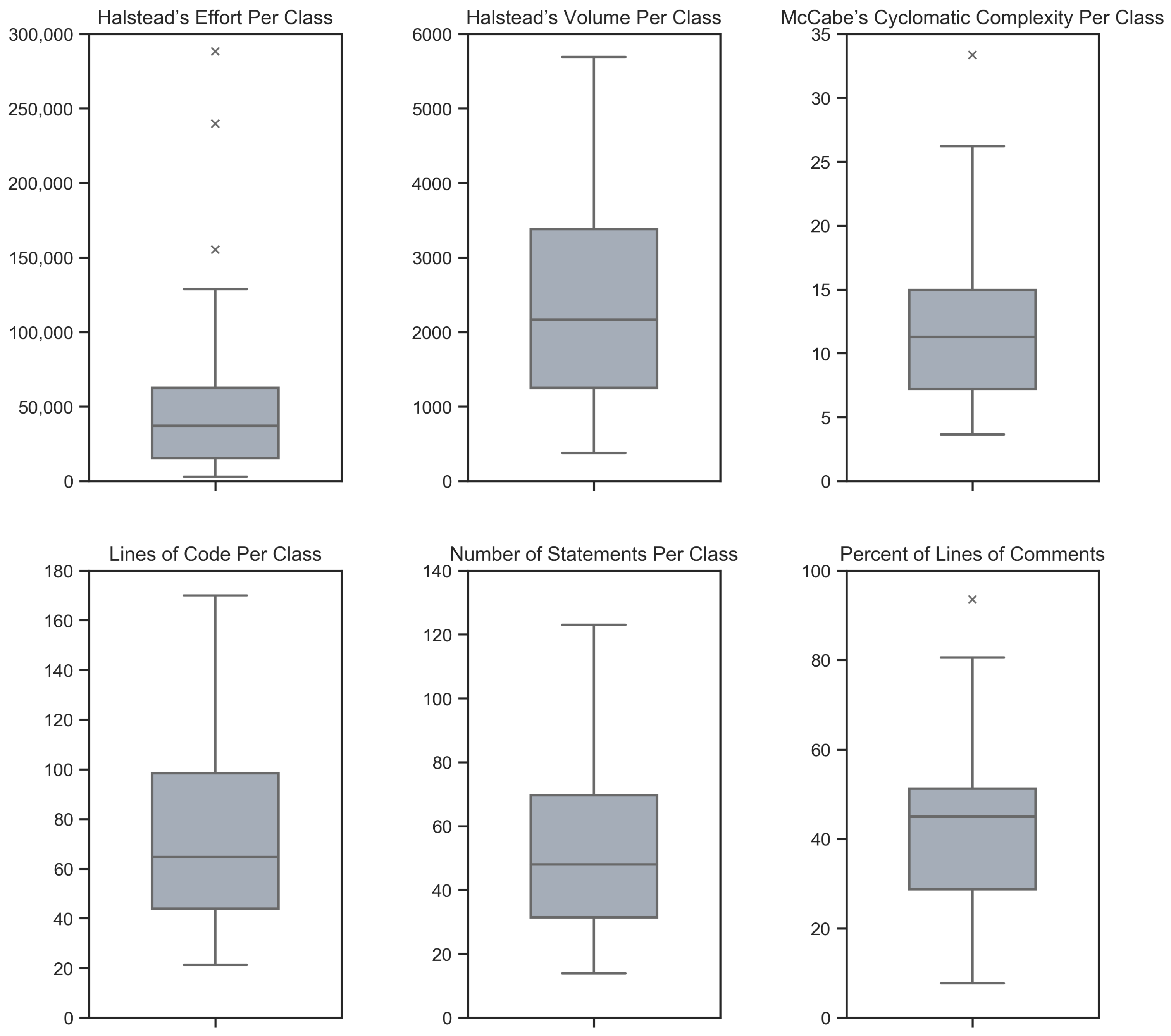
| Halstead’s Effort per Class | Halstead’s Volume per Class | McCabe’s Cyclomatic Complexity per Class | Lines of Code per Class | Number of Statements per Class | Percent of Lines of Comments | |
|---|---|---|---|---|---|---|
| Avg. | 54,201 | 2458 | 12.1 | 76.0 | 54.6 | 43.4 |
| Med. | 37,166 | 2164 | 11.3 | 64.6 | 47.9 | 44.9 |
| Std. | 58,992 | 1491 | 6.81 | 41.0 | 29.9 | 20.4 |
| Min. | 2957 | 377 | 3.64 | 21.3 | 13.9 | 7.64 |
| Max. | 288,226 | 5693 | 33.3 | 170 | 123 | 93.5 |
| Cohen’s d Effect Size | Interpretation of the Effect Magnitude |
|---|---|
| Very small effect | |
| Small effect | |
| Medium effect | |
| Large effect | |
| Very large effect | |
| Huge effect |
| Pearson’s Correlation | Kendall’s -b Correlation | Interpretation of the Correlation |
|---|---|---|
| Negligible correlation | ||
| Weak correlation | ||
| Moderate correlation | ||
| Strong correlation | ||
| Very strong correlation |
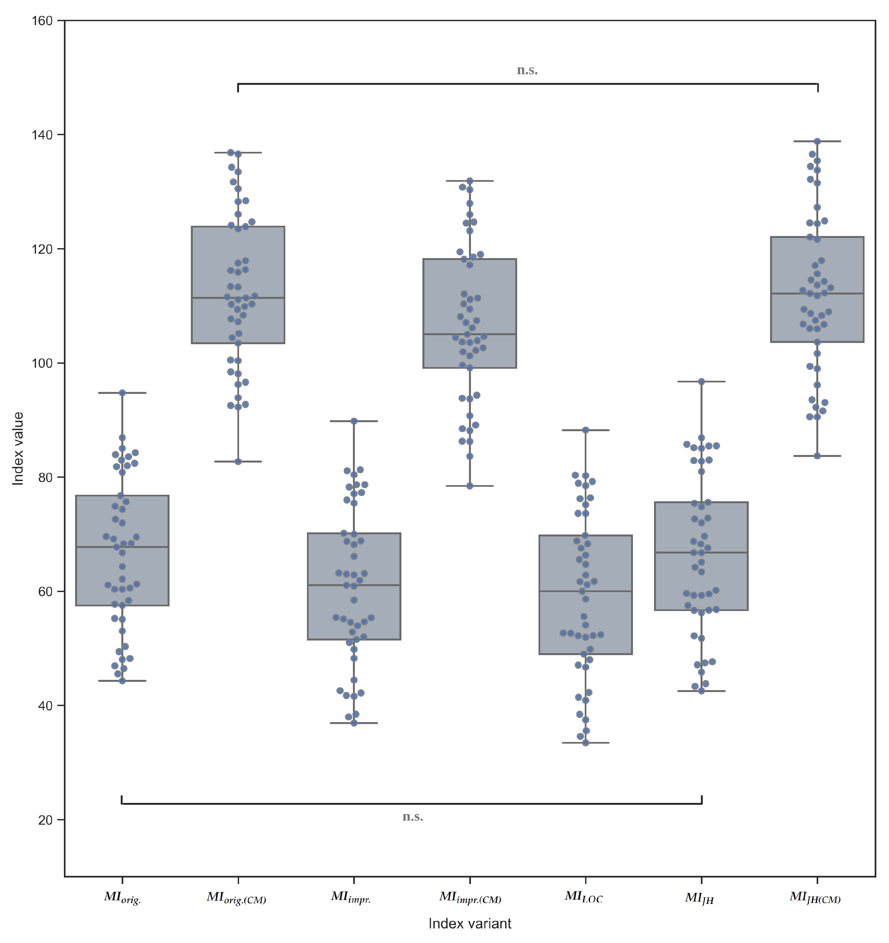
| MIorig. | MIorig.(CM) | MIimpr. | MIimpr.(CM) | MILOC | MIJH | MIJH(CM) | |
|---|---|---|---|---|---|---|---|
| Avg. | 66.66 | 112.41 | 60.90 | 106.64 | 59.23 | 66.37 | 112.11 |
| 95% CI | [62.64, 70.69] | [108.35, 116.47] | [56.73, 65.07] | [102.48, 110.8] | [54.87, 63.59] | [62.13, 70.61] | [107.87, 116.36] |
| Med. | 67.74 | 111.37 | 61.04 | 105 | 59.98 | 66.74 | 112.15 |
| Std. | 13.39 | 13.51 | 13.88 | 13.84 | 14.51 | 14.13 | 14.14 |
| Min. | 44.29 | 82.70 | 36.90 | 78.44 | 33.45 | 42.54 | 83.70 |
| Max. | 94.74 | 136.82 | 89.78 | 131.86 | 88.23 | 96.71 | 138.78 |
| Skew. | 0.06 | 0.03 | 0.06 | 0.04 | −0.01 | 0.10 | 0.08 |
| Kurt. | −1.00 | −0.69 | −0.93 | −0.72 | −0.97 | −0.90 | −0.68 |
| SW | W = 0.96, p = 0.147 | W = 0.98, p = 0.461 | W = 0.97, p = 0.207 | W = 0.97, p = 0.389 | W = 0.97, p = 0.256 | W = 0.96, p = 0.165 | W = 0.97, p = 0.352 |
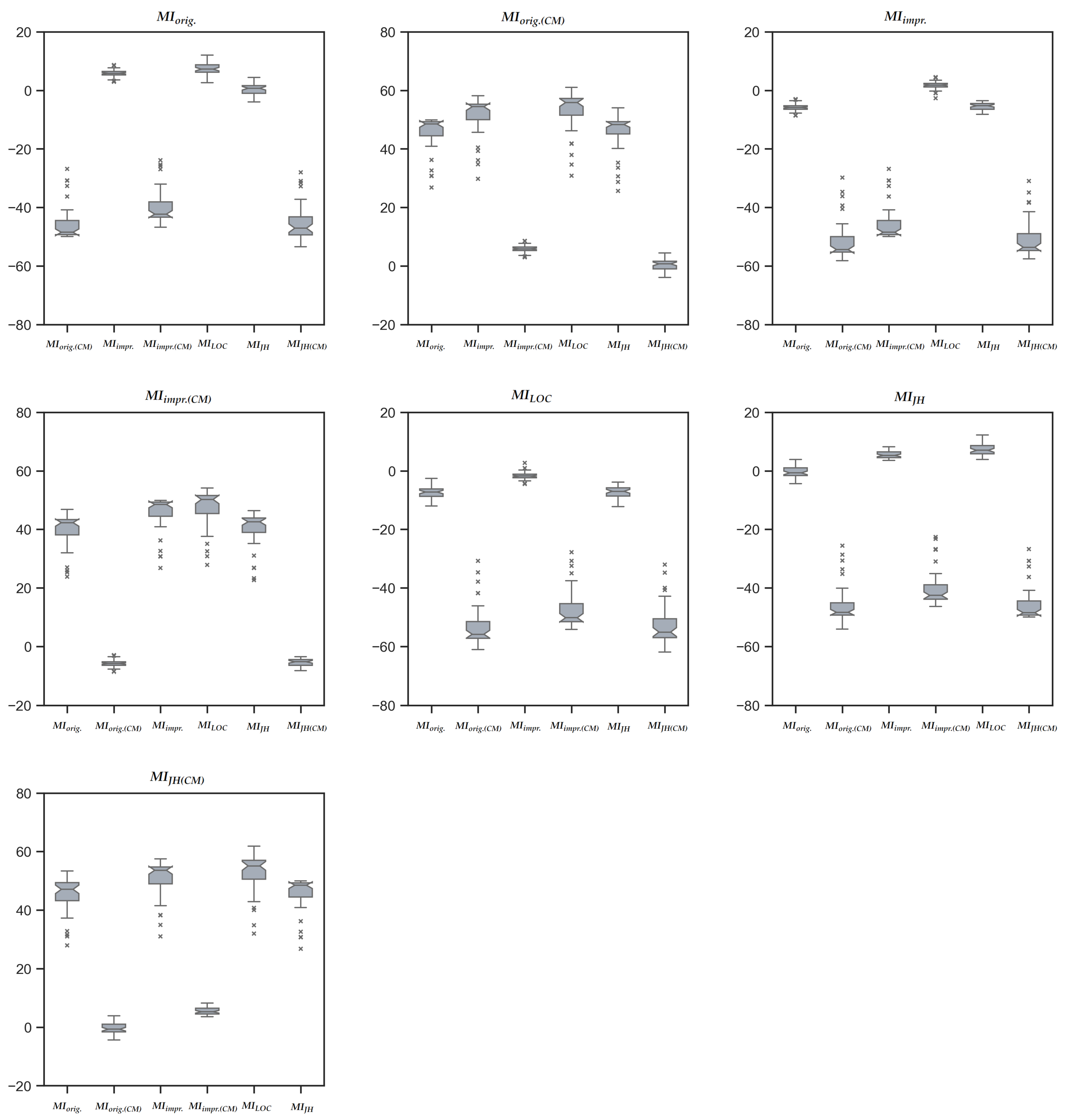
| Comparison Group | Reference Group | Shapiro–Wilk Normality Test | Avg.(±SE a/Med. b Difference | Test t a/Z b Value | Statistical Significance | Effect Size d a/rc b |
|---|---|---|---|---|---|---|
| MIorig. | MIorig.(CM) | W(45) = 0.71, p < 0.001 b | 48.50 | Z = −5.841 | p < 0.001 | rc = 1 |
| MIimpr. | W(45) = 0.95, p = 0.065 a | −5.77 ± 0.19 | t(44) = −30.54 | p < 0.001 | d = −4.55 | |
| MIimpr.(CM) | W(45) = 0.81, p < 0.001 b | 42.29 | Z = −5.841 | p < 0.001 | rc = 1 | |
| MILOC | W(45) = 0.99, p = 0.943 a | −7.43 ± 0.31 | t(44) = −23.88 | p < 0.001 | d = −3.56 | |
| MIJH | W(45) = 0.97, p = 0.363 a | −0.29 ± 0.27 | t(44) = −1.09 | p = 0.280 | d = −0.16 | |
| MIJH.(CM) | W(45) = 0.87, p < 0.001 b | 47.09 | Z = −5.841 | p < 0.001 | rc = 1 | |
| MIorig.(CM) | MIorig | W(45) = 0.71, p < 0.001 b | −48.50 | Z = −5.841 | p < 0.001 | rc = −1 |
| MIimpr. | W(45) = 0.74, p < 0.001 b | −54.40 | Z = −5.841 | p < 0.001 | rc = −1 | |
| MIimpr.(CM) | W(45) = 0.95, p = 0.065 a | −5.77 ± 0.19 | t(44) = −30.54 | p < 0.001 | d= −4.55 | |
| MILOC | W(45) = 0.82, p < 0.001 b | −55.84 | Z= −5.841 | p < 0.001 | rc= −1 | |
| MIJH | W(45) = 0.80, p < 0.001 b | −48.34 | Z = −5.841 | p < 0.001 | rc = −1 | |
| MIJH.(CM) | W(45) = 0.97, p = 0.363 a | −0.29 ± 0.27 | t(44) = −1.09 | p = 0.280 | d = −0.16 | |
| MIimpr. | MIorig | W(45) = 0.95, p = 0.065 a | 5.77 ± 0.19 | t(44) = 30.54 | p < 0.001 | d = 4.55 |
| MIorig.(CM) | W(45) = 0.74, p < 0.001 b | 54.40 | Z = −5.841 | p < 0.001 | rc = 1 | |
| MIimpr.(CM) | W(45) = 0.71, p < 0.001 b | 48.50 | Z = −5.841 | p < 0.001 | rc = 1 | |
| MILOC | W(45) = 0.95, p = 0.077 a | −1.67 ± 0.20 | t(44) = −8.42 | p < 0.001 | d = −1.26 | |
| MIJH | W(45) = 0.94, p = 0.023 b | 5.26 | Z = −5.841 | p < 0.001 | rc = 1 | |
| MIJH.(CM) | W(45) = 0.79, p < 0.001 b | 53.6 | Z = −5.841 | p < 0.001 | rc = 1 | |
| MIimpr.(CM) | MIorig | W(45) = 0.81, p < 0.001 b | −42.29 | Z = −5.841 | p < 0.001 | rc= −1 |
| MIorig.(CM) | W(45) = 0.95, p = 0.065 a | 5.77 ± 0.19 | t(44) = 30.54 | p < 0.001 | d = 4.55 | |
| MIimpr. | W(45) = 0.71, p < 0.001 b | −48.50 | Z = −5.841 | p < 0.001 | rc = −1 | |
| MILOC | W(45) = 0.79, p < 0.001 b | −50.20 | Z = −5.841 | p < 0.001 | rc = −1 | |
| MIJH | W(45) = 0.78, p < 0.001 b | −42.58 | Z = −5.841 | p < 0.001 | rc = −1 | |
| MIJH.(CM) | W(45) = 0.94, p = 0.023 b | 5.26 | Z = −5.841 | p < 0.001 | rc = 1 | |
| MILOC | MIorig | W(45) = 0.99, p = 0.943 a | 7.43 ± 0.31 | t(44) = 23.88 | p < 0.001 | d = 3.56 |
| MIorig.(CM) | W(45) = 0.82, p < 0.001 b | 55.84 | Z = −5.841 | p < 0.001 | rc = 1 | |
| MIimpr. | W(45) = 0.95, p = 0.077 a | 1.67 ± 0.20 | t(44) = 8.42 | p < 0.001 | d = 1.26 | |
| MIimpr.(CM) | W(45) = 0.79, p < 0.001 b | 50.20 | Z = −5.841 | p < 0.001 | rc = 1 | |
| MIJH | W(45) = 0.98, p = 0.576 a | 7.14 ± 0.29 | t(44) = 24.48 | p < 0.001 | d = 3.65 | |
| MIJH.(CM) | W(45) = 0.85, p < 0.001 b | 55.11 | Z = −5.841 | p < 0.001 | rc = 1 | |
| MIJH | MIorig | W(45) = 0.97, p = 0.363 a | 0.29 ± 0.27 | t(44) = 1.09 | p = 0.280 | d = 0.16 |
| MIorig.(CM) | W(45) = 0.80, p < 0.001 b | 48.34 | Z = −5.841 | p < 0.001 | rc = 1 | |
| MIimpr. | W(45) = 0.94, p = 0.023 b | −5.26 | Z = −5.841 | p < 0.001 | rc = −1 | |
| MIimpr.(CM) | W(45) = 0.78, p < 0.001 b | 42.58 | Z = −5.841 | p < 0.001 | rc = 1 | |
| MILOC | W(45) = 0.98, p = 0.576 a | −7.14 ± 0.29 | t(44) = −24.48 | p < 0.001 | d = −3.65 | |
| MIJH.(CM) | W(45) = 0.71, p < 0.001 b | 48.50 | Z = −5.841 | p < 0.001 | rc = 1 | |
| MIJH(CM) | MIorig | W(45) = 0.87, p < 0.001 b | −47.09 | Z = −5.841 | p < 0.001 | rc = −1 |
| MIorig.(CM) | W(45) = 0.97, p = 0.363 a | 0.29 ± 0.27 | t(44) = 1.09 | p = 0.280 | d = 0.16 | |
| MIimpr. | W(45) = 0.79, p < 0.001 b | −53.61 | Z = −5.841 | p < 0.001 | rc = −1 | |
| MIimpr.(CM) | W(45) = 0.94, p = 0.023 b | −5.26 | Z = −5.841 | p < 0.001 | rc = −1 | |
| MILOC | W(45) = 0.85, p < 0.001 b | −55.11 | Z = −5.841 | p < 0.001 | rc = −1 | |
| MIJH | W(45) = 0.71, p < 0.001 b | −48.50 | Z= −5.841 | p < 0.001 | rc= −1 |
| Case Study | MIorig. | MIorig.(CM) | MIimpr. | MIimpr.(CM) | MILOC | MIJH | MIJH(CM) |
|---|---|---|---|---|---|---|---|
| CS1. AssertJ | W = 0.151, p = 0.001 | W = 0.199, p < 0.001 | W = 0.189, p < 0.001 | W = 0.177, p < 0.001 | W = 0.159, p < 0.001 | W = 0.169, p < 0.001 | W = 0.255, p < 0.001 |
| CS2. Caffeine | W = 0.102, p = 0.186 | W = 0.131, p = 0.011 | W = 0.100, p = 0.200 | W = 0.137, p = 0.006 | W = 0.113, p = 0.050 | W = 0.091, p = 0.200 | W = 0.156, p < 0.001 |
| CS3. Joda-Time | W = 0.404, p < 0.001 | W = 0.395, p < 0.001 | W = 0.404, p < 0.001 | W = 0.399, p < 0.001 | W = 0.404, p < 0.001 | W = 0.404, p < 0.001 | W = 0.402, p < 0.001 |
| CS1. AssertJ | |||||||
|---|---|---|---|---|---|---|---|
| MIorig. | MIorig.(CM) | MIimpr. | MIimpr.(CM) | MILOC | MIJH | MIJH(CM) | |
| MIorig. | 1 | 0.919 | 0.942 | 0.870 | 0.805 | 0.729 | 0.724 |
| MIorig.(CM) | 0.919 | 1 | 0.873 | 0.943 | 0.745 | 0.663 | 0.789 |
| MIimpr. | 0.942 | 0.873 | 1 | 0.838 | 0.860 | 0.780 | 0.750 |
| MIimpr.(CM) | 0.870 | 0.943 | 0.838 | 1 | 0.716 | 0.630 | 0.813 |
| MILOC | 0.805 | 0.745 | 0.860 | 0.716 | 1 | 0.887 | 0.683 |
| MIJH | 0.729 | 0.663 | 0.780 | 0.630 | 0.887 | 1 | 0.667 |
| MIJH(CM) | 0.724 | 0.789 | 0.750 | 0.813 | 0.683 | 0.667 | 1 |
| CS2.Caffeine | |||||||
| MIorig. | MIorig.(CM) | MIimpr. | MIimpr.(CM) | MILOC | MIJH | MIJH(CM) | |
| MIorig. | 1 | 0.629 | 0.909 | 0.651 | 0.892 | 0.885 | 0.629 |
| MIorig.(CM) | 0.629 | 1 | 0.679 | 0.972 | 0.703 | 0.659 | 0.945 |
| MIimpr. | 0.909 | 0.679 | 1 | 0.700 | 0.948 | 0.864 | 0.663 |
| MIimpr.(CM) | 0.651 | 0.972 | 0.700 | 1 | 0.724 | 0.679 | 0.923 |
| MILOC | 0.892 | 0.703 | 0.948 | 0.724 | 1 | 0.864 | 0.685 |
| MIJH | 0.885 | 0.659 | 0.864 | 0.679 | 0.864 | 1 | 0.663 |
| MIJH(CM) | 0.629 | 0.945 | 0.663 | 0.923 | 0.685 | 0.663 | 1 |
| CS3.Joda-Time | |||||||
| MIorig. | MIorig.(CM) | MIimpr. | MIimpr.(CM) | MILOC | MIJH | MIJH(CM) | |
| MIorig. | 1 | 0.957 | 0.988 | 0.963 | 0.977 | 0.988 | 0.983 |
| MIorig.(CM) | 0.957 | 1 | 0.945 | 0.994 | 0.934 | 0.945 | 0.971 |
| MIimpr. | 0.988 | 0.945 | 1 | 0.951 | 0.984 | 0.988 | 0.971 |
| MIimpr.(CM) | 0.963 | 0.994 | 0.951 | 1 | 0.940 | 0.951 | 0.974 |
| MILOC | 0.977 | 0.934 | 0.984 | 0.940 | 1 | 0.980 | 0.963 |
| MIJH | 0.988 | 0.945 | 0.988 | 0.951 | 0.980 | 1 | 0.974 |
| MIJH(CM) | 0.983 | 0.971 | 0.971 | 0.974 | 0.963 | 0.974 | 1 |
| Case Study | MIorig. | MIorig.(CM) | MIimpr. | MIimpr.(CM) | MILOC | MIJH | MIJH(CM) |
|---|---|---|---|---|---|---|---|
| CS1. AssertJ | Z = −7.640, = −0.056, p < 0.001 | Z = −8.316, = −0.064, p < 0.001 | Z = −7.153, = −0.048, p < 0.001 | Z = −8.672, = −0.055, p < 0.001 | Z = −5.718, = −0.031, p < 0.001 | Z = −4.650, = −0.025, p < 0.001 | Z = −7.841, = −0.033, p < 0.001 |
| CS2. Caffeine | Z = −3.485, = −0.010, p < 0.001 | Z = −6.783, = −0.051, p < 0.001 | Z = −3.871, = −0.011, p < 0.001 | Z = −6.509, = −0.054, p < 0.001 | Z = −4.120, = −0.014, p < 0.001 | Z = −4.369, = −0.015, p < 0.001 | Z = −7.156, = −0.056, p < 0.001 |
| CS3. Joda-Time | Z = −9.302, = −0.030, p < 0.001 | Z = −9.276, = −0.032, p < 0.001 | Z = −9.302, = −0.032, p < 0.001 | Z = −9.276, = −0.034, p < 0.001 | Z = −9.234, = −0.037, p < 0.001 | Z = −9.334, = −0.024, p < 0.001 | Z = −9.324, = −0.027, p < 0.001 |
Disclaimer/Publisher’s Note: The statements, opinions and data contained in all publications are solely those of the individual author(s) and contributor(s) and not of MDPI and/or the editor(s). MDPI and/or the editor(s) disclaim responsibility for any injury to people or property resulting from any ideas, methods, instructions or products referred to in the content. |
© 2023 by the authors. Licensee MDPI, Basel, Switzerland. This article is an open access article distributed under the terms and conditions of the Creative Commons Attribution (CC BY) license (https://creativecommons.org/licenses/by/4.0/).
Share and Cite
Heričko, T.; Šumak, B. Exploring Maintainability Index Variants for Software Maintainability Measurement in Object-Oriented Systems. Appl. Sci. 2023, 13, 2972. https://doi.org/10.3390/app13052972
Heričko T, Šumak B. Exploring Maintainability Index Variants for Software Maintainability Measurement in Object-Oriented Systems. Applied Sciences. 2023; 13(5):2972. https://doi.org/10.3390/app13052972
Chicago/Turabian StyleHeričko, Tjaša, and Boštjan Šumak. 2023. "Exploring Maintainability Index Variants for Software Maintainability Measurement in Object-Oriented Systems" Applied Sciences 13, no. 5: 2972. https://doi.org/10.3390/app13052972