Research on Crack Width Measurement Based on Binocular Vision and Improved DeeplabV3+

Abstract

Crack width is the main manifestation of concrete material deterioration. To measure the crack information quickly and conveniently, a non-contact measurement method of concrete planar structure crack based on binocular vision is proposed. Firstly, an improved DeeplabV3+ semantic segmentation model is proposed, which uses L-MobileNetV2 as the backbone feature extraction network, adopts IDAM structure to extract high-level semantic information, introduces ECA attention mechanism, and optimizes the loss function of the model to achieve high-precision segmentation of crack areas. Secondly, the plane space coordinate equation of the concrete structure was constructed based on the principle of binocular vision and SIFT feature point matching, and the crack width was calculated by combining the segmented image. Finally, to verify the performance of the above method, a measurement test platform was built. The experimental results show that the RMSE of the crack measurement by using the algorithm is less than 0.2 mm, and the error rate is less than 4%, which has stable accuracy in different measurement angles. It solves the problem of fast and convenient measurement of the crack width of concrete planar structures in an outdoor environment.

1. Introduction

Concrete material is widely used in construction engineering, such as roads, bridges, walls, and so on. The crack width on the surface of the concrete structure directly reflects its degradation degree and bearing capacity. Regular detection of cracks plays an important role in the maintenance and operation of existing infrastructure and buildings.

Traditional crack measurement is mainly carried out by inspectors using crack scales or magnifying glasses, which is time-consuming, tedious, and subjective [1]. With the development of technology, crack detection systems based on fiber optic sensors, laser, stereo imaging, ultrasonic and other technologies have been developed [2,3], but these systems are often very expensive. For roads, bridges, and other large detection areas, many institutions are unable to use these methods for regular inspection of cracks in the concrete surface, usually only one inspection a year, leading to their inability to timely evaluate the safety situation, resulting in a lot of accidents due to the deterioration of the road, and bridge deck structure. Compared with the above technology, the measurement method based on visual inspection technology has the advantages of non-contact and low hardware cost [4,5]. Therefore, in recent years, the vision-based crack measurement method has gradually become a hot research topic. The overall process is divided into two steps: detection and coordinate transformation.

Traditional image crack detection algorithms include morphological methods, edge detection methods, and statistics-based methods [6], but these methods have low detection accuracy in noisy images. At present, crack detection methods using deep learning are widely used, and their detection methods mainly include two kinds: anchor-based object detection algorithm and semantic segmentation algorithm. Kang et al. [7] used Fast RCNN to extract the crack area in the panoramic image with an anchor box and processed the image in the area to obtain the length and width of the crack. However, the noise existing in the anchor box still affected the subsequent crack boundary extraction [8,9]. At present, many studies on crack segmentation based on semantic segmentation models such as FCN [10,11,12], U-Net [13,14,15,16,17], PSPNet [18], and Deeplab series [19,20] have emerged, which verify the effectiveness of semantic segmentation models for crack extraction. However, the segmentation accuracy of these models needs to be improved. High-precision segmentation of the crack edge is helpful to reduce the image processing steps before subsequent measurement, and improve the automation level and the final measurement accuracy. As the new peak of semantic segmentation, the DeeplabV3+ model has high accuracy in most datasets. But because of the imbalance of samples in the crack dataset and the sparsity of the model’s high semantic receptive field, the model often performs poorly in crack segmentation experiments.

After the crack edge is accurately extracted, most studies on crack measurement based on visual pixel position have used a camera in the past, which requires that the optical axis of the camera should be perpendicular to the crack surface. When the detection distance and angle change, it needs to be re-calibrated [21,22], which makes mobile deployment difficult. To this end, Zhao [23] used a single camera and a laser range finder to ensure real-time calibration of parameters, but the error will increase sharply when the angle between the camera and the object surface exceeds 50°. In contrast, binocular vision measurement establishes the spatial relationship between the camera and the object through left-right image matching and coordinate transformation and does not need to re-calibrate when the distance and angle between the camera and the object change [24,25,26]. However, due to the mismatching that often occurred in the current stereo-matching algorithm, the accuracy of the edge measurement is often not high.

Aiming at the problem that the current semantic model is not accurate enough for crack segmentation and the left and right images of binocular cameras are mismatched, resulting in large errors. In this paper, an improved DeeplabV3+ model is proposed to achieve more accurate crack segmentation. Secondly, the coordinates of the crack edge space points were obtained according to the feature point matching, and the precise measurement accuracy was obtained under different angles combined with the segmentation image.

2. Crack Region Segmentation Algorithm

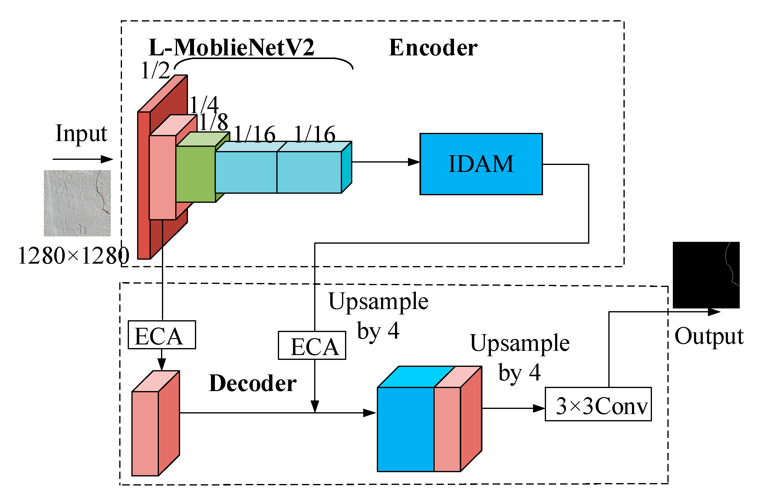
2.1. Improved DeeplabV3+ Algorithm

In this paper, we choose to improve on the DeeplabV3+ semantic segmentation model to achieve higher segmentation accuracy for crack regions. The improvements include the following four areas:

(1)

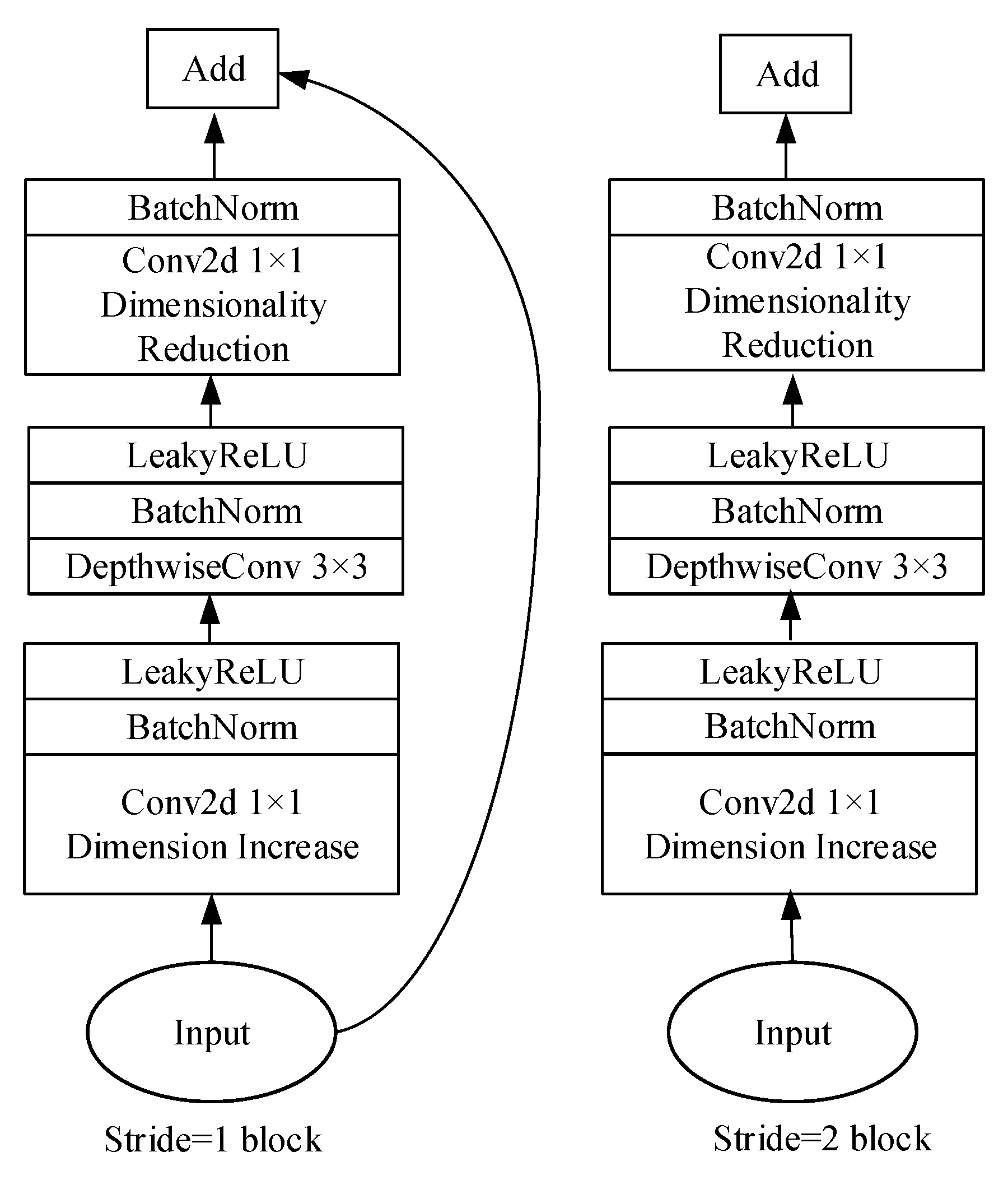
Modify the Xception feature extraction network to the L-MobileNetV2 network structure.

(2)

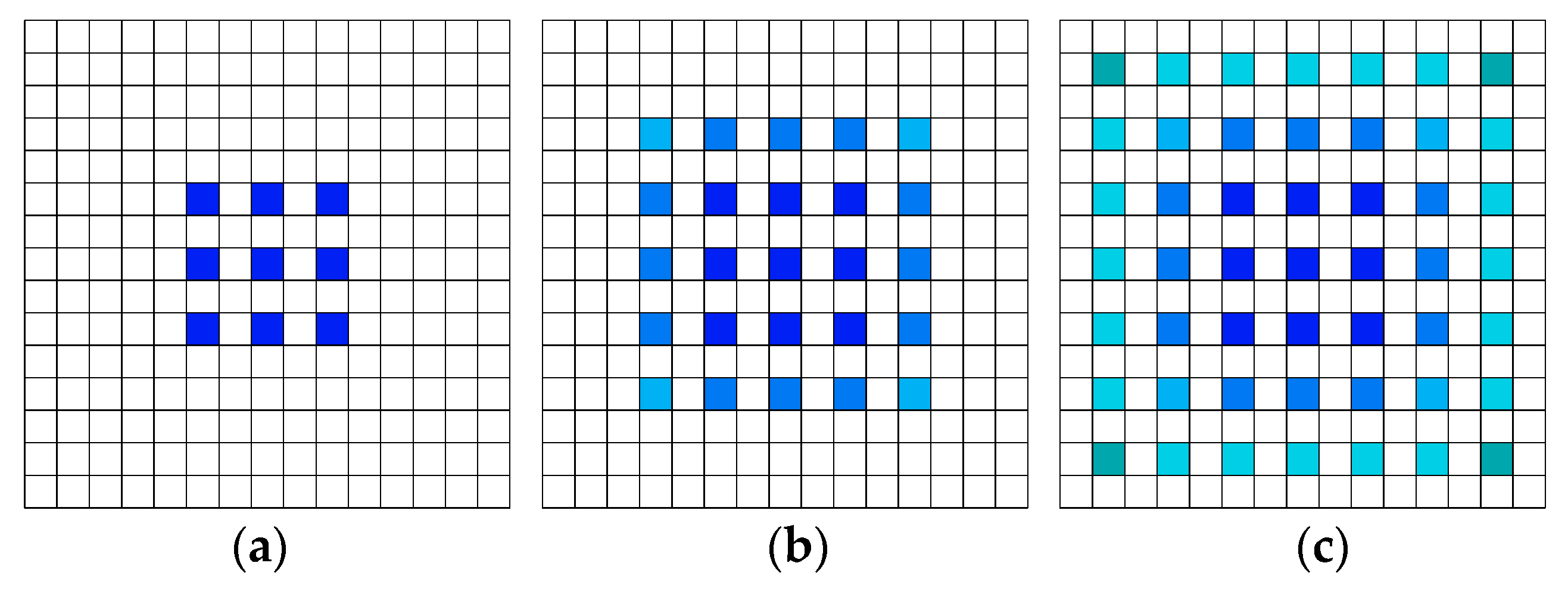
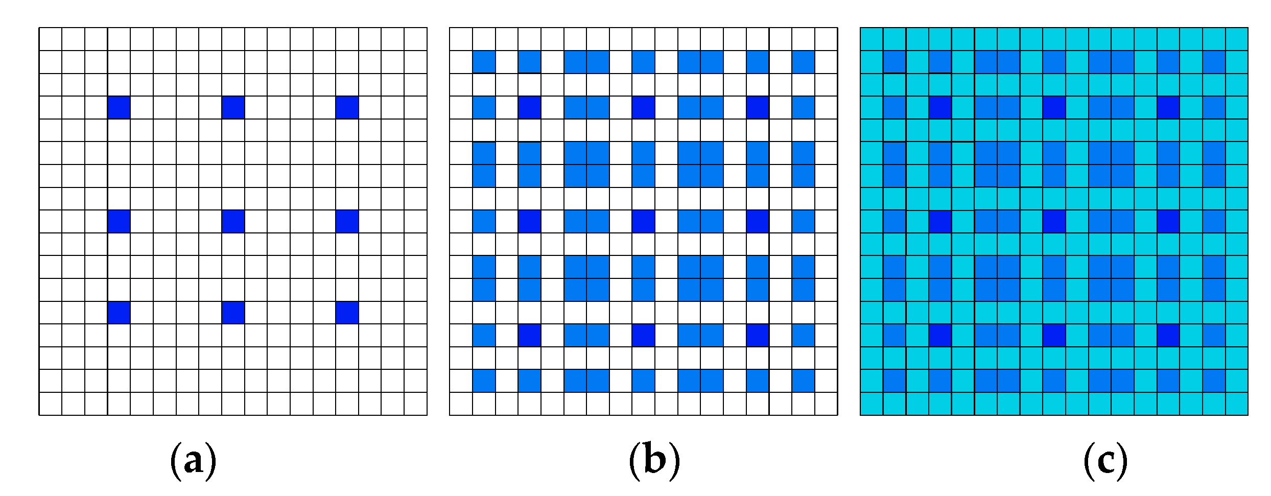
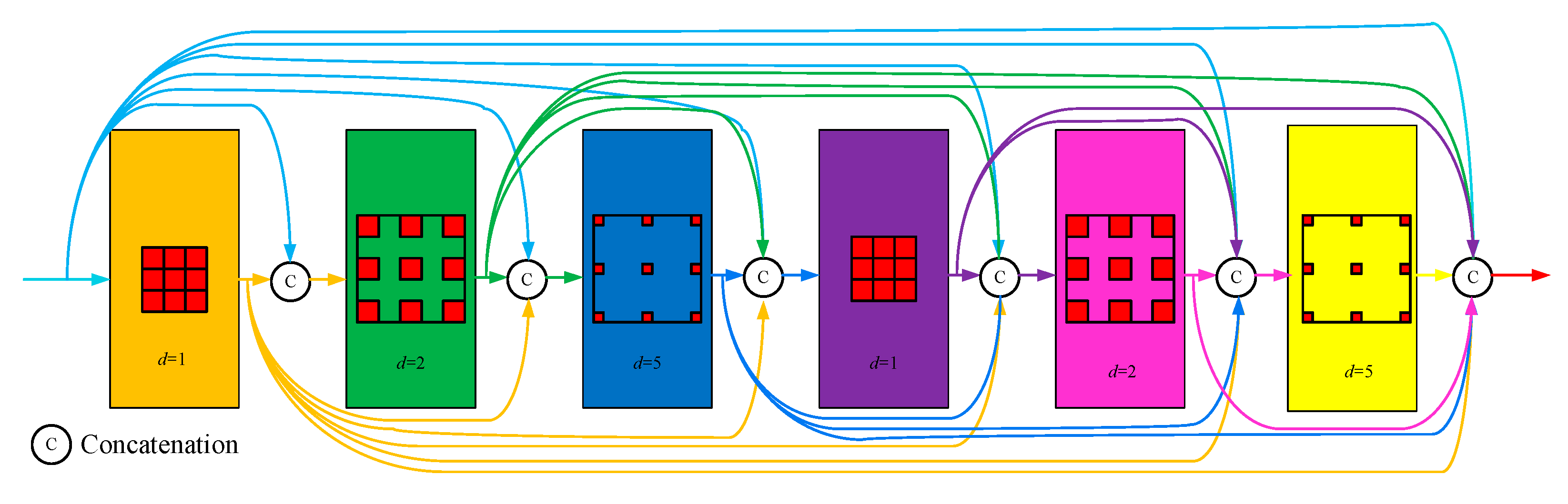
According to the HDC (Hybrid Dilated Convolution) strategy, an improved DenseASPP module (IDAM) is designed to replace the ASPP (Atrous Spatial Pyramid Pooling) structure in the original model.

(3)

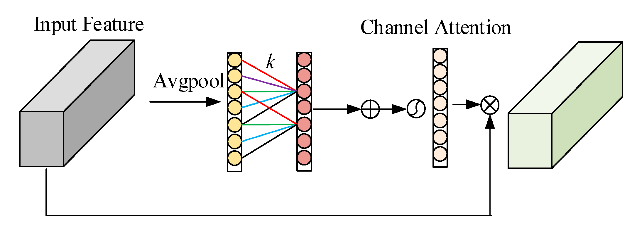
ECA (Efficient Channel Attention) mechanism is introduced to modulate the weight of channel information before splicing 1/4 shallow feature layers and 1/16 deep semantic information.

(4)

Introducing Focal loss and Dice loss functions to optimize the loss function.

The improved DeeplabV3+ model network structure is shown in Figure 1.

2.2. L-MobileNetV2

The original DeeplabV3+ model uses Xception as the backbone feature extraction network, but the Xception model has a large parameter scale and poor operation speed control. Therefore, this paper chooses the backbone network based on MobileNetV2 [27] to facilitate training and reduce detection time.

The ReLU activation function used in MobileNetV2 can alleviate the phenomenon of gradient dispersion. However, with the increase in network depth and the number of training rounds, some weights cannot be updated effectively due to the disappearance of the gradient, resulting in the phenomenon of neuron death. As a result, the average value of ReLU output is greater than 0, which is not conducive to the feature extraction ability of the network model. Therefore, this paper chooses to replace the activation function in MobileNetV2 with Leakey ReLU, which initializes neurons by giving negative output values a small slope, increases the extraction of negative value features, and avoids neuron death. Its mathematical expression is as follows.

$$y_i=\{\begin{array}{l}{x}_i,\hspace{1em}{x}_i\ge 0\\ \frac{x_i}{a_i},\hspace{0.17em}\hspace{0.17em}\hspace{0.17em}{x}_i<0\end{array}$$

(1)

where x_i represents the output of layer i, y_i represents the output after the nonlinear transformation of layer i, a_i is the hyperparameter in the Leakey ReLU activation function, and the default value is 100.

MobileNetV2 continues the depthwise separable convolution operation in the V1 version and introduces the inverted residual module and the linear bottleneck structure to increase the pair of features. The inverted residual module first uses 1 × 1 convolution to increase the dimension and then uses 3 × 3 convolution layer by layer to extract features across feature points and then uses 1 × 1 convolution to reduce the dimension. This process is the reverse of the residual extraction module of the ResNet network. The linear bottleneck structure is that the linear activation function is used in the convolution layer of the last layer of the inverted residual structure. Experiment [27] shows that this structure has a better feature recognition effect. The L-MobileNetV2 bottleneck residual module after the improved activation function is shown in Figure 2.

2.3. IDAM

The ASPP structure of the original DeeplabV3+ model uses the dilated convolution with expansion rates of 3, 6, 18, and 24 in parallel to extract the feature relationships of images under different receptive fields. However, when the dilated rate is greater than 24, the dilated convolution will gradually lose the feature extraction ability. Therefore, Yang et al. adopted dilated convolution with expansion rates of 3, 6, 12, 18, and 24 to replace the parallel feature extraction structure of ASPP by dense connection, and proposed a DenseASPP model [28], which obtained more and larger receptive fields. However, this method still has the problem of the checkerboard effect, that is, it is assumed that the dilated convolution with convolution kernel size 3 and expansion rate 2 is used to perform three consecutive operations on the image, and the covering points are marked with blue. The extracted pixels are shown in Figure 3. As can be seen from the white squares in the figure, the correlation between local information is destroyed and the information is seriously lost.

To this end, the HDC strategy is adopted in this paper, that is, dilated convolutions with different expansion rates are used alternately and continuously to reduce the influence of the checkerboard effect [29]. Suppose that when there are N dilated convolutional layers with kernel size ksize, the dilation rate is {d₁,…, d_i, …, d_n}, define the maximum distance between two non-zero points as follows.

$$M_i=MAX[M_{i+1}-2d_i,M_{i+1}-2(M_{i+1}-d_i),d_i]$$

(2)

where M_n = d_n, HDC strategy requires M₂ ≤ ksize. When ksize = 3 and d = {1,2,5}, M₂ = MAX [1,−1,2] = 2 ≤ 3, HDC strategy is satisfied. The convolution extraction result is shown in Figure 4, which shows that this connection strategy can effectively use image information and weaken the checkerboard effect.

To obtain enough and large enough receptive fields, the convolution kernel with an expansion rate of {1,2,5} is designed to be used twice in this paper. The IDAM model structure is shown in Figure 5:

Bring the current structure into the receptive field calculation formula:

$$\{\begin{array}{l}RF=(d-1)\times (ksize-1)+ksize\\ R{F}_n=R{F}_{n-1}+k_n-1\end{array}$$

(3)

In the formula, RF_n represents the receptive field of the n-layer dilated convolution, k_n is the size of the n-layer dilated convolution, and the maximum receptive field size of IDAM is [2 × 2 × (1 + 2 + 5) + 1] = 33. It is sufficient to process the 1/16 (80 × 80 pixels) depth feature map input in the trunk network. Compared with the four receptive field combinations of ASPP structure, according to the permutation combination, the number of extracted feature combinations of IDAM can be calculated as follows:

$$N_{IDAM}={\displaystyle \sum _{m=1}^{n=6}{C}_n^m=63}$$

(4)

It can be seen that the IDAM model structure obtains more combined high-level semantic features.

2.4. ECA Attention Mechanism

In the original DeeplabV3+ model, channels were stacked directly between the 1/4 shallow feature layer and the deep feature layer through the ASPP structure, and the importance of semantic information obtained by each channel was the same by default. However, with the increase of network depth and the expansion of the receptive field, semantic information would gradually decrease and enrich. The importance of each channel feature is also different. IDAM structure used in this paper has more channels than ASPP, so it is necessary to modulate the weight of each channel.

Based on SE (Squeeze-and-Excitation) attention mechanism, the efficient channel attention mechanism [30] uses 1d convolution to replace the fully connected layer after average pooling to compress the features of each channel, which not only reduces the number of parameters, but also avoids the introduction of redundant channel dependencies. After that, the Sigmoid function is used to compress the weights to between 0 and 1. Finally, the input feature map and the processed weights are multiplied to form the features after modulating the channel weights, as shown in Figure 6.

In the figure, k is the optimal range of channel information interaction, that is, the convolution kernel size of 1d convolution, which is calculated as Equation (5):

$$k={\left|\frac{{\log }_2(C)}{\mathsf{\gamma }}+\frac{b}{\mathsf{\gamma }}\right|}_{odd}$$

(5)

where, C is the number of characteristic channels, and γ and b are generally set to 2 and 1.

The final channel attention ω is calculated as follows:

$$\omega =\sigma (C1D_{\mathrm{k}}\left(\mathrm{AvgPool}\right(\mathrm{F}\left)\right)$$

(6)

where F is the input feature, C1D_k represents the 1d convolution with convolution kernel k, and σ represents the Sigmoid function.

2.5. Loss Function Modification

In the obtained crack images, the pixel area occupied by the vast majority of cracks is smaller than the background area. This situation will lead to the imbalance of positive and negative samples in the training process of the algorithm, cause the weight shift, and lead to a poor crack segmentation effect. Based on this situation, this paper uses the combination of Dice loss and Focal loss to replace the cross-entropy loss function to solve the problem of extremely unbalanced samples in the data set, where the expression of Dice loss is as follows:

$$Dice loss=1-\frac{2{\displaystyle {\sum }_{i=1}^N{y}_i{y^{\prime }}_i}}{{\displaystyle {\sum }_{i=1}^N{y}_i}+{\displaystyle {\sum }_{i=1}^N{y^{\prime }}_i}}$$

(7)

where, y_i and y′_i represent the label value and the predicted value of pixel i respectively, and N is the total number of pixels.

The Focal loss is expressed as follows.

$$Focal\hspace{0.17em}loss=-\alpha {(1-p_t)}^{\beta }\log (p_t)$$

(8)

where, α is used to adjust the ratio of positive and negative sample loss, and the weight of the background region in the loss function of the model can be reduced by setting the value of α, which is set as 0.5 in this paper. β is an adjustable factor, which is used to improve the emphasis of the algorithm on the training of difficult samples for crack extraction. In this paper, 2 is taken, and p_t represents the probability that the predicted pixel is a crack.

Finally, the loss function in the DeeplabV3+ model is improved as follows.

$$Loss=Dice loss+Focal\hspace{0.17em}loss$$

(9)

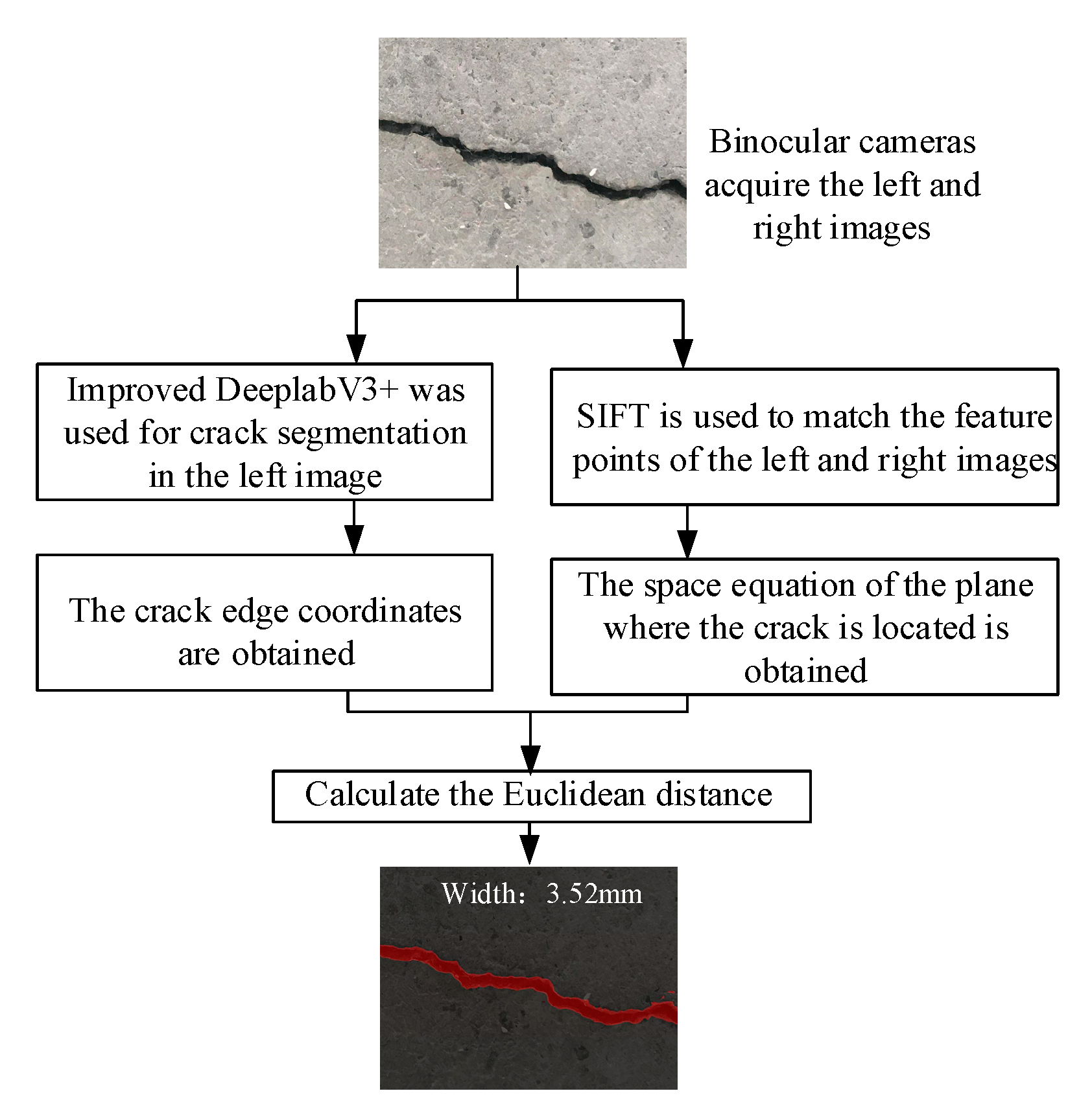
3. Visual Method for Measuring Crack Width in Concrete

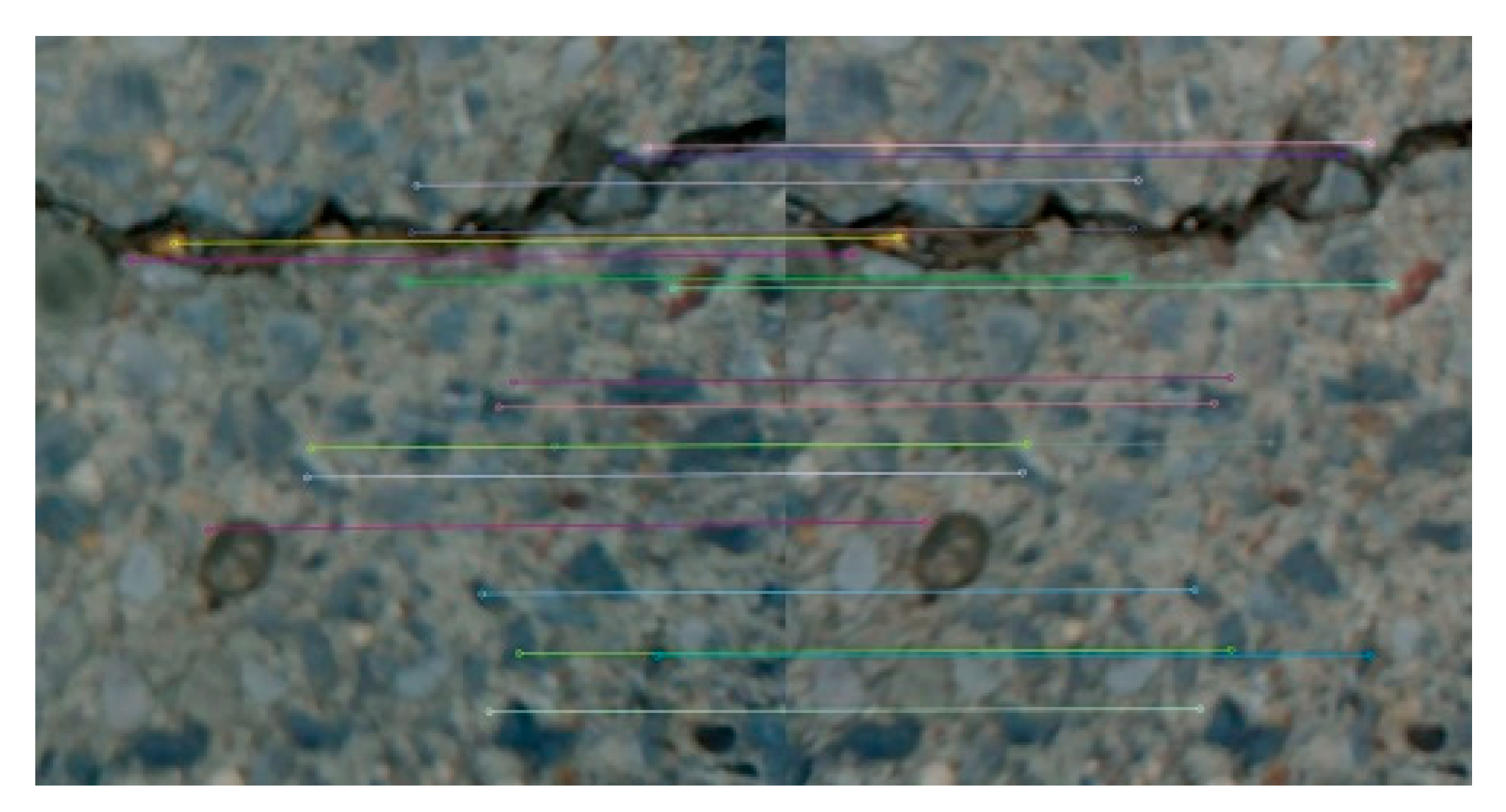
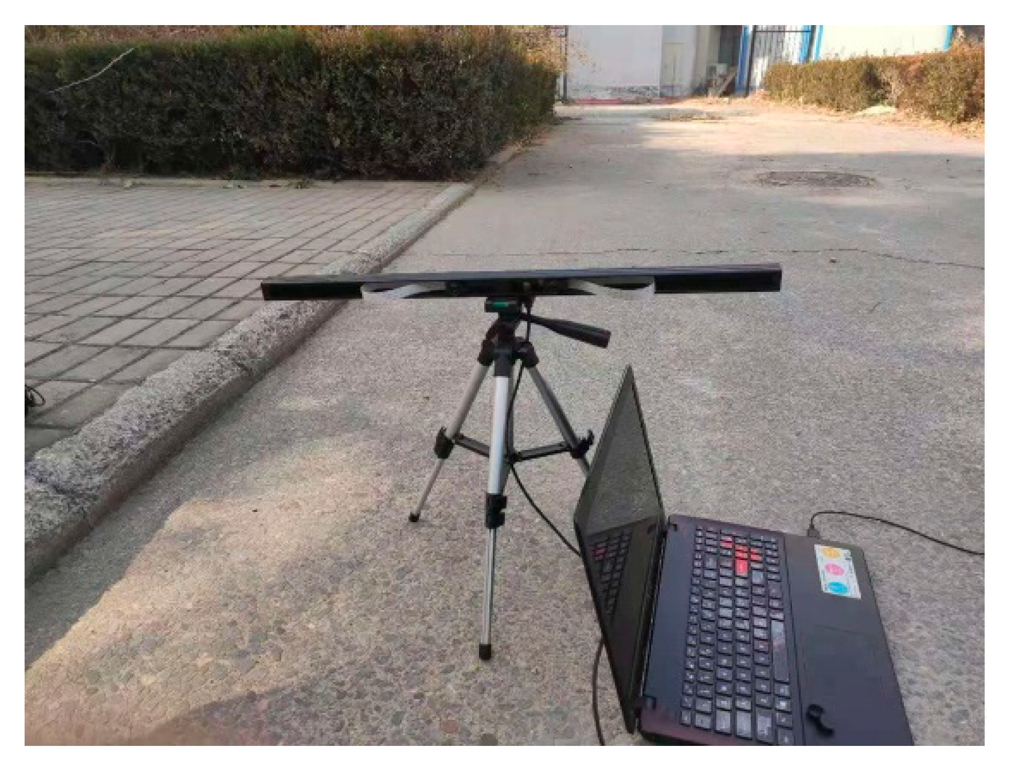
3.1. Binocular Vision Spatial Coordinate Acquisition Algorithm

Binocular vision obtains the spatial information of objects by matching the left and right camera images. Global matching and semi-global matching algorithms are commonly used, but these methods will produce a large number of mismatching regions in the matching process, resulting in holes. In this paper, an algorithm based on only three matching feature points to establish the space equation for crack measurement is designed for the case that the cracks of concrete are mostly in the plane region.

The measurement principle of binocular vision is based on the parallax theory, that is, if P is a point in space, the spatial coordinates are (X, Y, Z), p_L and p_R are the imaging points of the target P on the left and right cameras, and the image coordinates are (x_l, y_l), (x_r, y_r) respectively, then the calculation method of the spatial coordinates of P is as follows.

$$\{\begin{array}{l}X=d\cdot x_l/x_l-x_r\\ Y=d\cdot y_l/x_l-x_r\\ Z=d\cdot f/x_l-x_r\end{array}$$

(10)

where f is the focal length of the camera and d is the baseline length of the binocular camera.

Since the SIFT feature point matching algorithm is robust to noise and illumination, this paper relies on it to match the feature points of the left and right crack images. As shown in Figure 7, it can be seen that the matching accuracy of the left and right image feature points of this method is high.

The three points with the highest matching similarity of feature points are selected as the concrete plane space equation, as shown in Figure 8, O represents the optical center of the left camera, O_LX_LY_L is the imaging plane of the left camera, O_wX_wY_w is the spatial structure plane, p is a point on the crack edge of the spatial plane represented by the blue curve. Suppose that the coordinates of three non-collinear spatial points are p₁(X₁,Y_1,Z₁), p₂(X₂,Y_2,Z₂), and p₃(X₃,Y_3,Z₃).

Therefore, the normal vector n of the structural plane where the crack is located can be solved by the following equation:

$$\{\begin{array}{l}\overrightarrow{p_1{p}_2}=(X_2-X_1,X_2-Y_1,Z_2-Z_1)\\ \overrightarrow{p_1{p}_3}=(X_3-X_1,Y_3-Y_1,Z_3-Z_1)\\ \overrightarrow{n}=\overrightarrow{p_1{p}_2}\times \overrightarrow{p_1{p}_3}\end{array}$$

(11)

Then the structural plane equation is expressed as follows.

$$(X-X_1,Y-Y_1,Z-Z_1)\cdot \overrightarrow{n}=0$$

(12)

Combined with Equation (10), the corresponding relationship between each pixel in the left image and the spatial coordinates can be finally obtained.

3.2. Crack Parameter Acquisition Algorithm

In the routine inspection and maintenance of concrete structures, the maximum crack width is usually used to evaluate the damage to the structure. In this paper, firstly, the centerline position of the crack in the image is obtained according to the skeleton extraction algorithm, and the crack edge area is divided according to the skeleton. The maximum crack width is taken as the shortest distance from any point on one edge of the crack to the other side of the crack, and its expression is as follows:

$$\begin{array}{l}{w}_i=\min (\sqrt{{(X_i-X_j)}^2+{(Y_i-Y_j)}^2+{(Z_i-Z_j)}^2})\\ \hspace{1em}\hspace{1em}i,j=1,2,3\dots ,n\end{array}$$

(13)

3.3. Measurement Process of Crack Parameters

In this paper, using the above crack detection and binocular vision algorithm, combined with the experimental platform in Chapter 4, a crack parameter measurement method is proposed. Firstly, the concrete plane with cracks is captured by a binocular camera, and the left camera image is input into the improved DeeplabV3+ algorithm to segment the crack area, and the image coordinates of the crack boundary are input into the List. Then, the SIFT algorithm was used to match the feature points of the left and right images, and the coordinate transformation relationship between the left image pixels and the space plane was calculated by combining the calibrated internal and external parameters of the camera. Finally, each point in List was traversed according to Equation (13), and the spatial Euclidean distance was calculated to obtain the maximum width of the crack. The above process is shown in Figure 9.

4. Experiment and Analysis

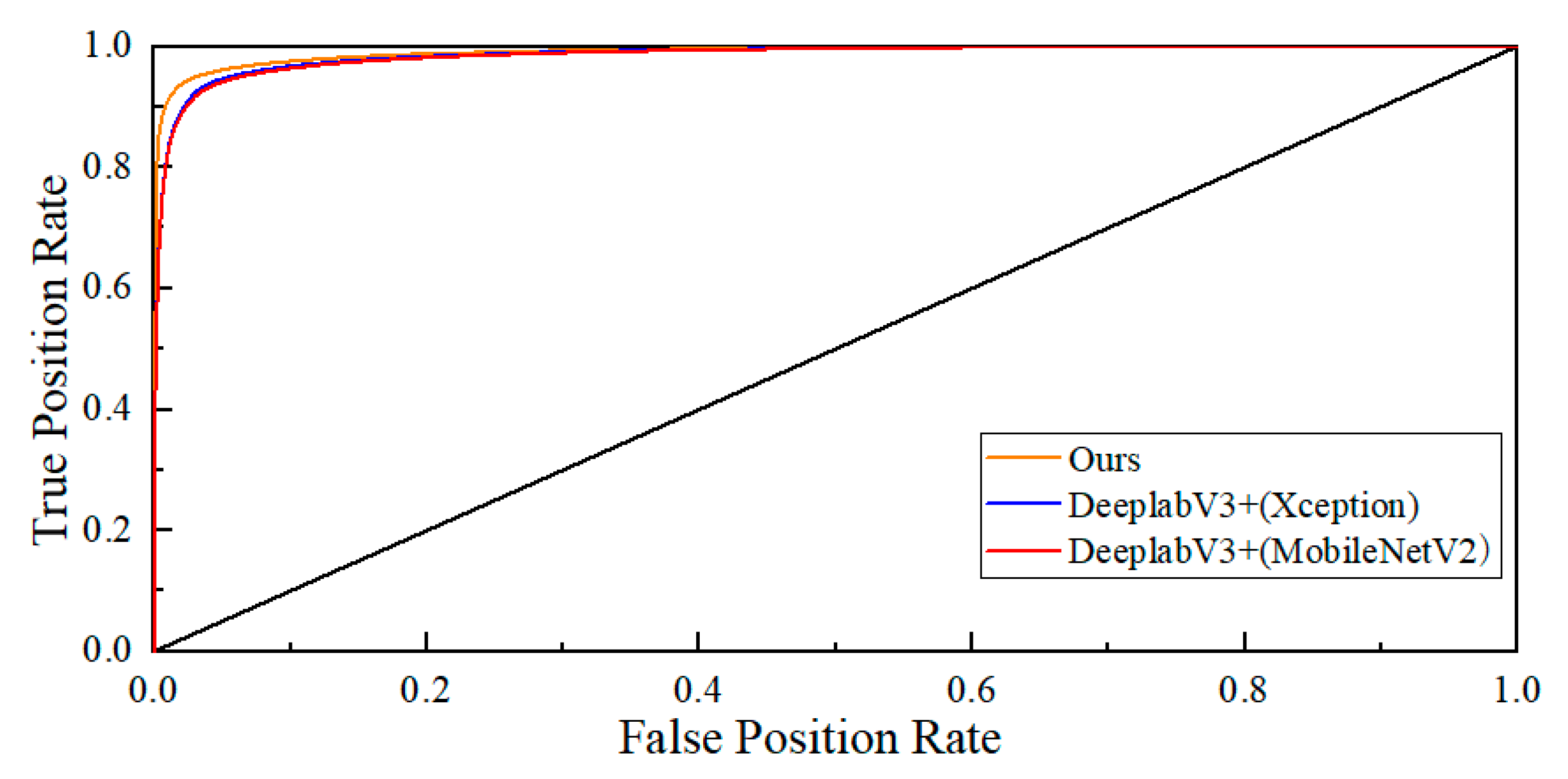
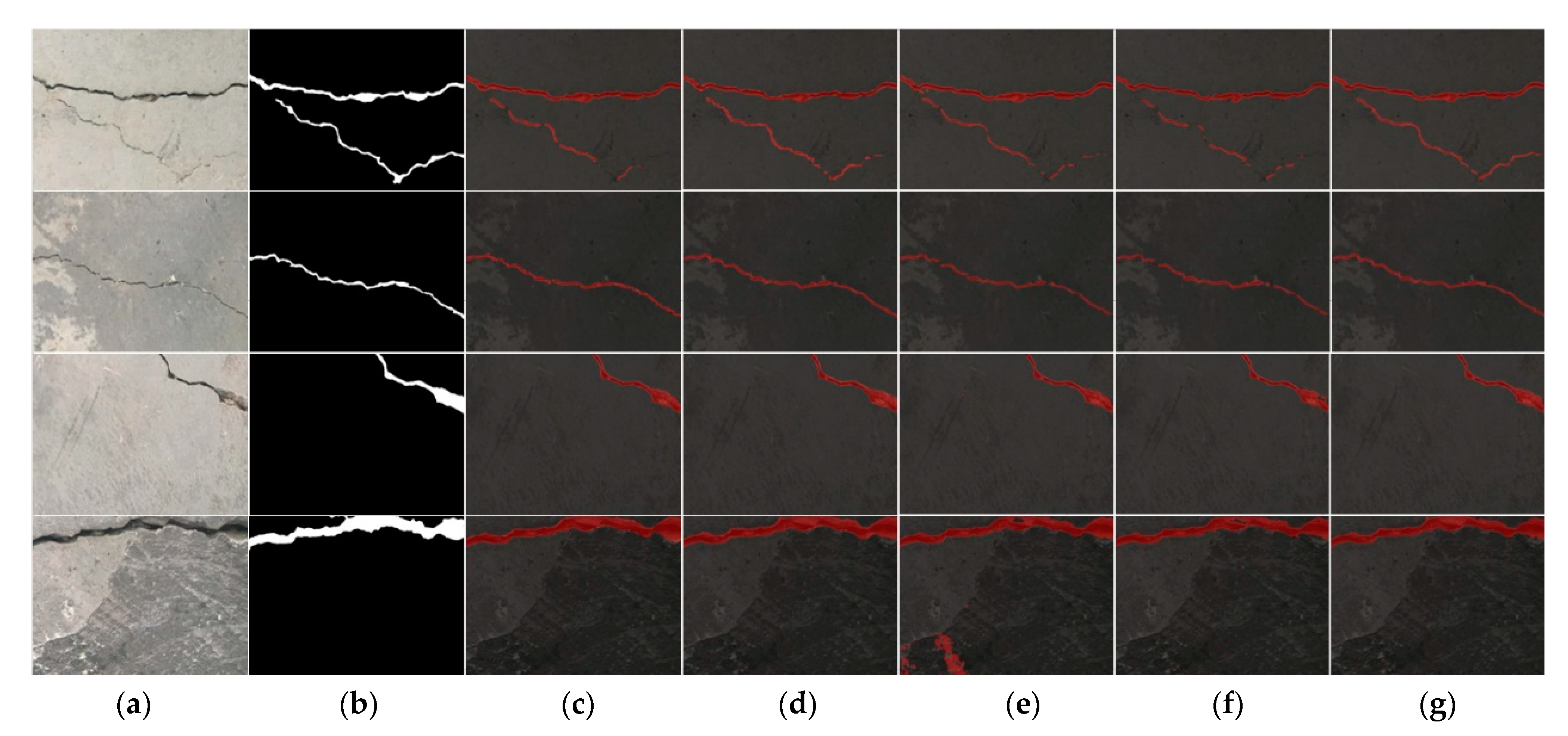
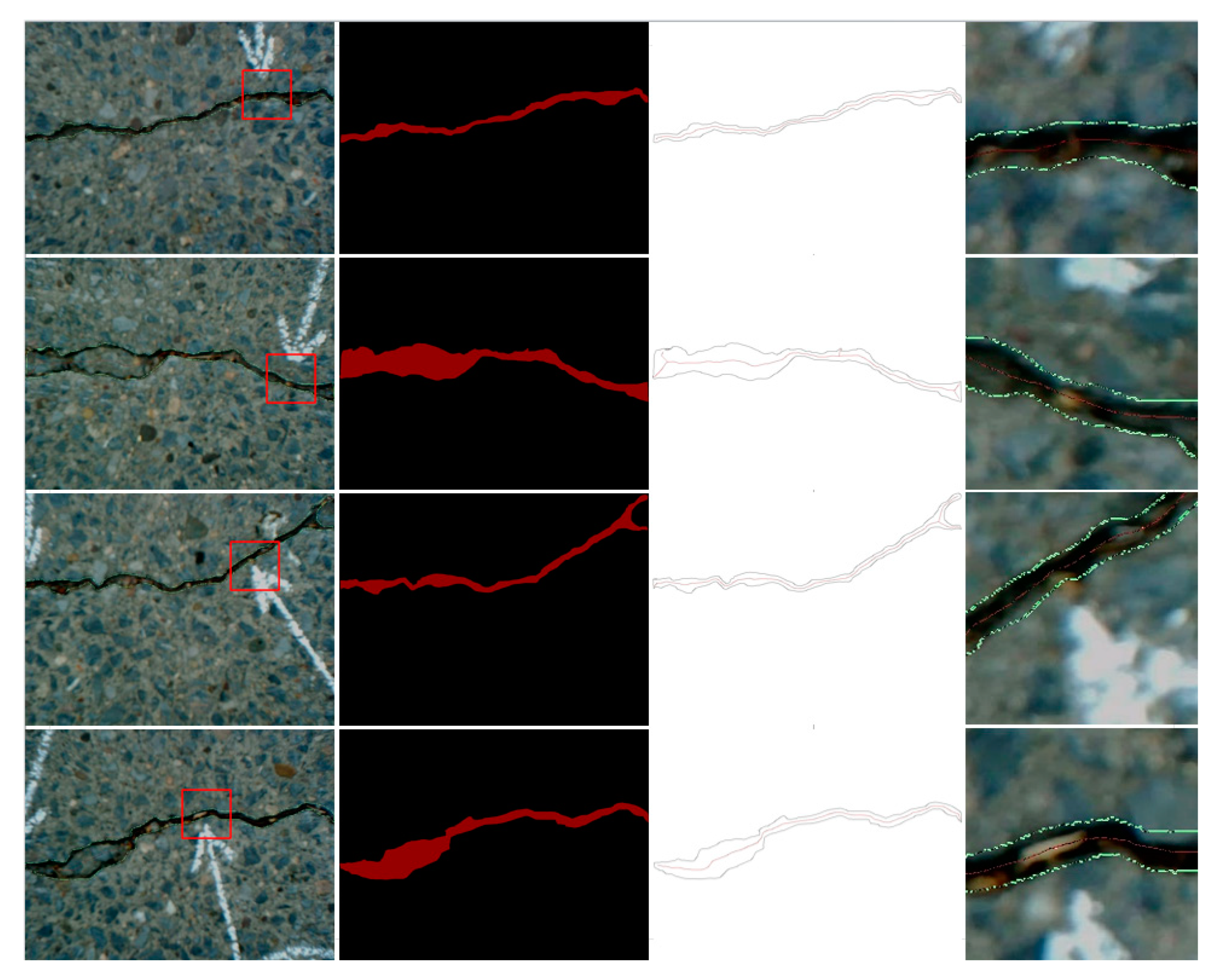
4.1. Improved DeeplabV3+ Algorithm Verification Experiment

The data set in this paper is 1466 high-resolution crack images obtained from Internet search and field shooting and enhanced by data. The training set, verification set, and test set are divided in a ratio of 8:1:1. Crack segmentation model training was based on Python language, Pytorch framework, and PyCharm integrated development platform, and the experimental GPU was GeForce RTX 3060.

In the training process, the model is divided into two parts. First, the backbone network is trained by freezing 60 epochs, and then it is trained by thawing 140 epochs to accelerate the training speed of the model. The batch size of the frozen part is 8, and the batch size of the unfrozen part is 4. Cosine annealing is used to reduce the learning rate. The change in loss value in the training process is shown in Figure 10.

To verify the effectiveness of the crack segmentation model proposed in this paper, the improved DeeplabV3+ model and the current mainstream segmentation models are respectively used to train the crack data set made in this paper. Different models use the same training set, verification set, and test set. The performance of each model is evaluated by model parameter size, Mean Intersection over Union (MIoU), Mean Pixel Accuracy (MPA), and Pixel Accuracy (PA). At the same time, to prove the rationality of the improved method in this paper, the DeeplabV3+ model with Xception and MobileNetV2 as the backbone feature extraction network is also added to participate in the comparison, as shown in

Table 1. Performance comparison of different segmentation models.

Network Model	MIoU	MPA	PA	Parameter Size
PSPNet	85.90%	90.74%	99.08%	2.376M
HRNet	84.96%	89.91%	98.92%	9.637M
U-Net	87.02%	90.26%	99.12%	24.891M
DeeplabV3+(Xception)	88.70%	93.67%	99.18%	54.709M
DeeplabV3+(MobileNetV2)	88.79%	92.28%	99.23%	5.813M
Ours	92.26%	95.54%	99.45%	16.833M

. To further compare the ability of these models to identify cracks, their ROC curves were fitted using a B-spline curve by adjusting the confidence threshold, as shown in Figure 11.

Table 1 shows that the DeeplabV3+ model is higher than other models in the Accuracy indicators of MIoU, MPA, and Accuracy. Combined with Figure 11, we can see that the predictive power of the original DeeplabV3+ model with Xception as the backbone network is similar to the model with MobileNetV2. However, the original DeeplabV3+ model parameter size is about 9.4 times that of the latter. The parameter size of the improved DeeplabV3+ model proposed in this paper is about 1/3 that of the original model, and its ROC curve is higher than the original model. Compared with the original model, the MIoU, MPA, and PA of the improved model are increased by 3.56%, 1.87%, and 0.27%. The segmentation results of different models are shown in Figure 12.

As can be seen from Figure 12, PSPNet, U-Net, and the original DeeplabV3+ models are prone to generate breakpoints when segmenting cracks, resulting in discontinuous cracks. U-Net model is easy to identify holes on the concrete surface as cracks and has a high mismatching rate. Although HRNet generated fewer breakpoints in the face of small cracks, it can be seen from the third and fourth-row images that the model segmented the crack edge relatively wide. From the comparison of the first and second-row images, it can be seen that the proposed method can effectively extract continuous narrow cracks with fewer fractures. By comparing the labeled images with the segmentation images of different models, it can be seen that the proposed method is the most accurate for extracting the crack region.

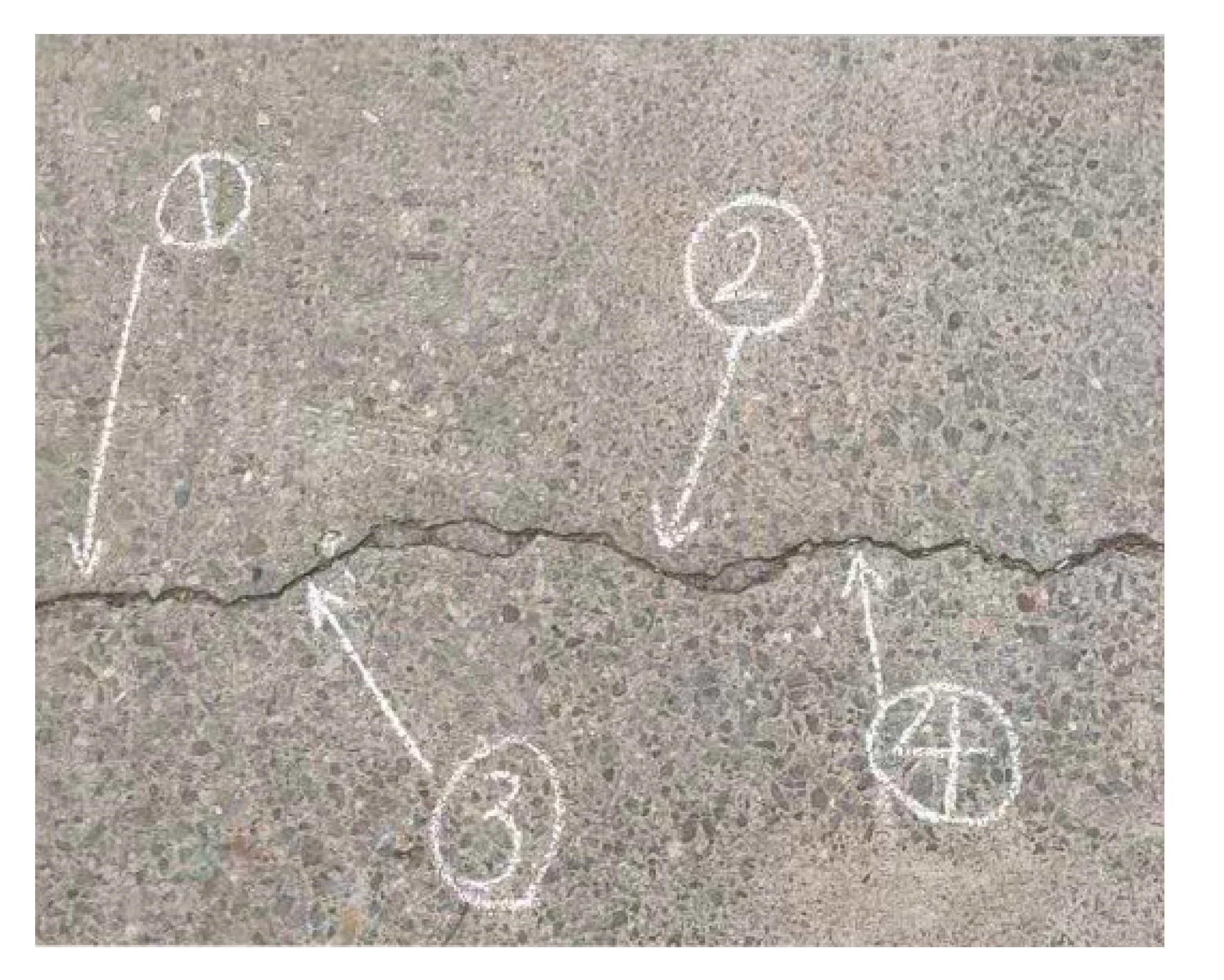
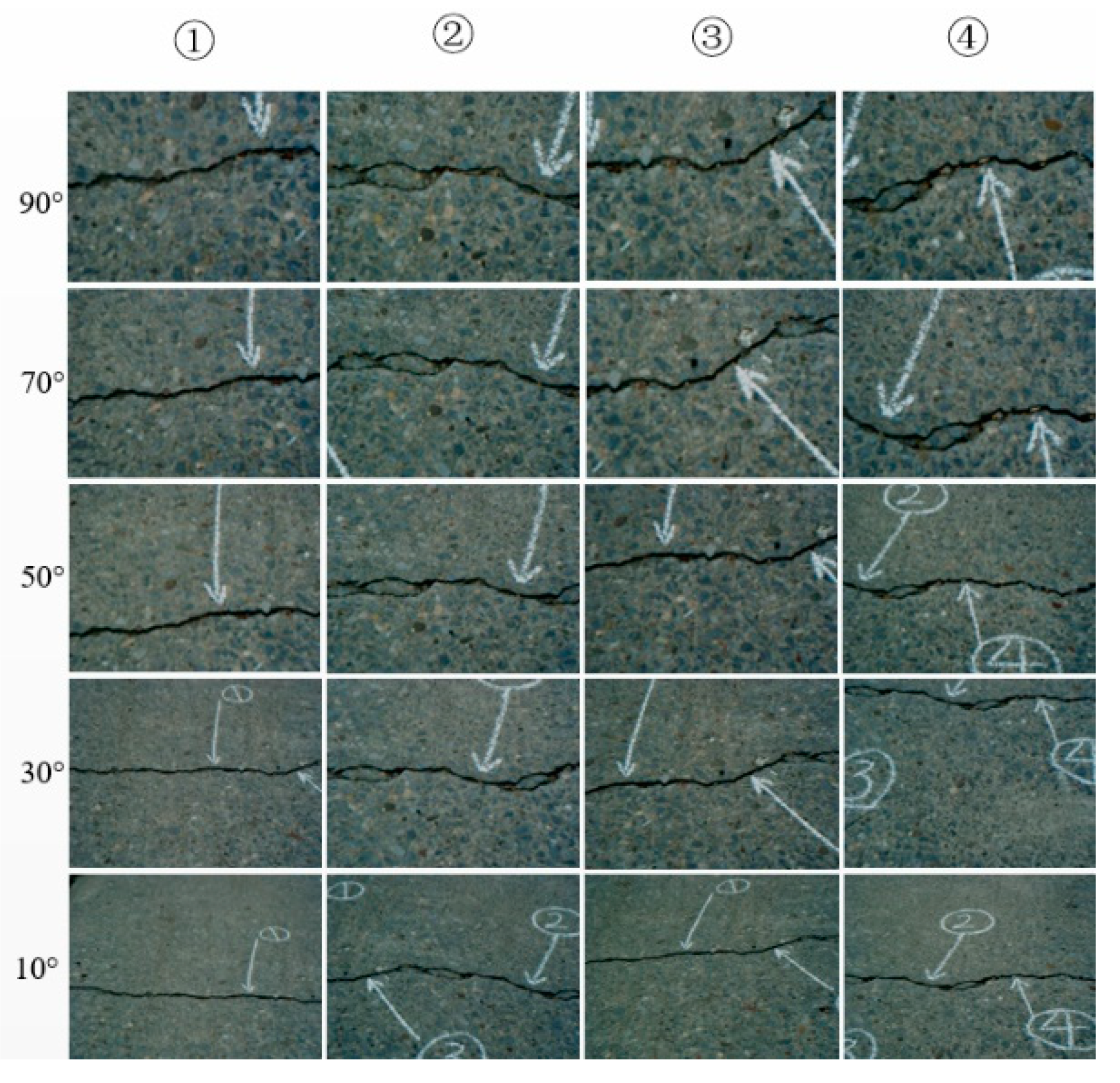
4.2. Crack Measurement Experiment

In this section, the concrete crack width measurement method proposed in this paper is experimentally verified. The AYALEY adjustable baseline binocular camera is used in the experiment, and its maximum resolution is 1280 × 960, as shown in Figure 13. Before measurement, the camera calibration toolbox in MATLAB is used to calculate the internal and external parameters of the camera.

The experiment chooses to measure the crack of concrete pavement, and Figure 14 shows the four positions selected for the measurement.

The central axis of the camera was made perpendicular to the concrete pavement for shooting, and the crack width was obtained by segmentation, edge extraction, and skeleton extraction of the four crack images respectively, as shown in Figure 15. The fourth column is the edge and skeleton extraction effect in the first red box, which shows that the crack edge extracted by the proposed algorithm is more accurate.

To verify the accuracy of the proposed crack width measurement method, the measurement comparison experiment is carried out, as shown in

Table 2. Crack width measurement error.

ID	True Value/mm	Results of Method 1/mm	Error Value/mm	Rate of Error/%	Results of Method 2/mm	Error Value/mm	Rate of Error/%	Results of Method 3/mm	Error Value/mm	Rate of Error/%
1	5.412	6.025	+0.613	11.33	5.876	+0.464	8.57	5.586	+0.174	3.22
2	4.210	4.412	+0.202	4.80	4.366	+0.156	3.71	4.085	−0.125	2.97
3	3.567	3.775	+0.208	5.83	3.238	−0.329	9.22	3.696	+0.129	3.62
4	6.189	5.023	−1.166	18.84	5.848	−0.341	5.51	6.321	+0.132	2.13

. Methods 1, 2, and 3 represent the original DeeplabV3+ algorithm combined with the semi-global matching method, the original DeeplabV3+ algorithm combined with the proposed spatial coordinate acquisition method, and the improved DeeplabV3+ method combined with the proposed spatial coordinate acquisition method, respectively. HICHANCE-CK101 crack width measuring instrument (Measurement accuracy: 0.01 mm) was used to calculate the true value of the crack width by the average of three measurements.

It can be seen from the measurement results in Table 2 that the absolute value of the error measured by method 1 to method 3 in this paper is gradually reduced, which verifies the effectiveness of the improved DeeplabV3+ algorithm and the space coordinate conversion algorithm proposed in this paper. Both of them can reduce the measurement error of the crack width, and the error rate of method 3 is less than 4% and the error value is less than 0.2 mm. To further prove the characteristics of easy deployment and stable measurement of this method, by fine-tuning the distance, the optical axis of the camera is adjusted to 90, 70, 50, 30, and 10 degrees from the concrete plane respectively. In this process, the left and right cameras were kept level, and the above 4 cracks were photographed and measured, as shown in Figure 16.

The error values measured by different angles of the four crack locations using the proposed measurement method are shown in

Table 3. Measurement errors at different angles.

ID	Measurement Error Value/mm
	10°	30°	50°	70°	90°
1	0.205	0.190	−0.188	−0.164	0.174
2	0.198	−0.176	0.171	0.152	−0.125
3	−0.210	0.184	0.165	−0.144	0.129
4	0.182	−0.187	0.126	0.152	0.132
RMSE	0.199	0.184	0.164	0.153	0.141

.

As can be seen from Table 3, with the reduction of the angle between the optical axis and the concrete plane, the measurement error of the crack width increases, and the RMSE of the crack measurement rises from 0.141 under the angle of 90° to 0.199 under the angle of 10°, but, in general, the error value is still small and the fluctuation is relatively gentle, which verifies the stability and effectiveness of the proposed method under different angles.

5. Conclusions

In this paper, the improved DeeplabV3+ model is used to extract the crack area in the panoramic image, and then obtain the edge of the crack in the segmentation map. The SIFT algorithm is used to match the three feature points of the original left and right images, and the conversion relationship between the image coordinates and the spatial coordinates is calculated to obtain the crack width information. Experiments on concrete pavement show that the method can measure the crack width on a concrete plane accurately. The main conclusions of this study are as follows:

(1)

The improved DeeplabV3+ model using the L-MobileNetV2 backbone network, IDAM module, ECA attention mechanism, and modified loss function can segment the crack area in the image more accurately than the current mainstream segmentation models. The MIoU, MPA, and PA of the model are 92.26%, 95.54%, and 99.45%, respectively.

(2)

Experimental results show that the method proposed in this paper has good measurement accuracy on the surface of the concrete structure. The error value of crack width measurement is less than 0.2 mm, and the error rate is less than 4%. Changing the angle between the camera optical axis and the concrete plane to measure the crack under 90 degrees to 10 degrees, it is found that the measured crack width RMSE increases with the decrease of the angle, but is not higher than 0.2 mm.

(3)

The proposed method is easy to deploy and improves crack detection efficiency. In the future, it can be integrated into a mobile automation platform to replace manual work and realize the regular detection of cracks on concrete pavements, bridges, and other surfaces. At the same time, without changing the resolution, the theoretical error of binocular vision measurement will increase rapidly with the increase in distance, and the current system cannot guarantee the accuracy of long-distance measurement.

References

1. Mohan, A.; Poobal, S. Crack detection using image processing: A critical review and analysis. Alex. Eng. J. 2018, 57, 787–798. [Google Scholar] [CrossRef]
2. Van Steen, C.; Nasser, H.; Verstrynge, E.; Wevers, M. Acoustic emission source characterisation of chloride-induced corrosion damage in reinforced concrete. Struct. Health Monit. 2022, 21, 1266–1286. [Google Scholar] [CrossRef]
3. Ye, Y.; Hu, S.; Fan, X.; Lu, J. Effect of adhesive failure on measurement of concrete cracks using fiber Bragg grating sensors. Opt. Fiber Technol. 2022, 71, 102934. [Google Scholar] [CrossRef]
4. Ma, Y.; Wu, Y.; Li, Q.; Zhou, Y.; Yu, D. ROV-based binocular vision system for underwater structure crack detection and width measurement. Multimed. Tools Appl. 2022, 1–25. [Google Scholar] [CrossRef]
5. Tang, Y.; Huang, Z.; Chen, Z.; Chen, M.; Zhou, H.; Zhang, H.; Sun, J. Novel visual crack width measurement based on backbone double-scale features for improved detection automation. Eng. Struct. 2023, 274, 115158. [Google Scholar] [CrossRef]
6. Tong, Z.; Gao, J.; Han, Z.; Wang, Z. Recognition of asphalt pavement crack length using deep convolutional neural networks. Road Mater. Pavement Des. 2018, 19, 1334–1349. [Google Scholar] [CrossRef]
7. Kang, D.; Benipal, S.S.; Gopal, D.L.; Cha, Y.J. Hybrid pixel-level concrete crack segmentation and quantification across complex backgrounds using deep learning. Autom. Constr. 2020, 118, 103291. [Google Scholar] [CrossRef]
8. Shahrokhinasab, E.; Hosseinzadeh, N.; Monirabbasi, A.; Torkaman, S. Performance of image-based crack detection systems in concrete structures. J. Soft Comput. Civ. Eng. 2020, 4, 127–139. [Google Scholar]
9. Lin, C.S.; Chen, S.H.; Chang, C.M.; Shen, T.W. Crack detection on a retaining wall with an innovative, ensemble learning method in a dynamic imaging system. Sensors 2019, 19, 4784. [Google Scholar] [CrossRef] [Green Version]
10. Chen, F.C.; Jahanshahi, M.R. NB-FCN: Real-time accurate crack detection in inspection videos using deep fully convolutional network and parametric data fusion. IEEE Trans. Instrum. Meas. 2019, 69, 5325–5334. [Google Scholar] [CrossRef]
11. Zhang, J.; Lu, C.; Wang, J.; Wang, L.; Yue, X.G. Concrete cracks detection based on FCN with dilated convolution. Appl. Sci. 2019, 9, 2686. [Google Scholar] [CrossRef] [Green Version]
12. Dung, C.V. Autonomous concrete crack detection using deep fully convolutional neural network. Autom. Constr. 2019, 99, 52–58. [Google Scholar] [CrossRef]
13. Lau, S.L.; Chong, E.K.; Yang, X.; Wang, X. Automated pavement crack segmentation using u-net-based convolutional neural network. IEEE Access 2020, 8, 114892–114899. [Google Scholar] [CrossRef]
14. Hsieh, Y.A.; Tsai, Y.J. Machine learning for crack detection: Review and model performance comparison. J. Comput. Civ. Eng. 2020, 34, 04020038. [Google Scholar] [CrossRef]
15. Su, H.; Wang, X.; Han, T.; Wang, Z.; Zhao, Z.; Zhang, P. Research on a U-Net Bridge Crack Identification and Feature-Calculation Methods Based on a CBAM Attention Mechanism. Buildings 2020, 12, 1561. [Google Scholar] [CrossRef]
16. Liu, Z.; Cao, Y.; Wang, Y.; Wang, W. Computer vision-based concrete crack detection using U-net fully convolutional networks. Autom. Constr. 2019, 104, 129–139. [Google Scholar] [CrossRef]
17. Li, G.; Ma, B.; He, S.; Ren, X.; Liu, Q. Automatic tunnel crack detection based on u-net and a convolutional neural network with alternately updated clique. Sensors 2020, 20, 717. [Google Scholar] [CrossRef] [Green Version]
18. Wang, J.J.; Liu, Y.F.; Nie, X.; Mo, Y.L. Deep convolutional neural networks for semantic segmentation of cracks. Struct. Control Health Monit. 2022, 29, e2850. [Google Scholar] [CrossRef]
19. Sun, X.; Xie, Y.; Jiang, L.; Cao, Y.; Liu, B. DMA-Net: DeepLab With Multi-Scale Attention for Pavement Crack Segmentation. IEEE Trans. Intell. Transp. Syst. 2022, 23, 18392–18403. [Google Scholar] [CrossRef]
20. Li, Z.; Zhu, H.; Huang, M. A deep learning-based fine crack segmentation network on full-scale steel bridge images with complicated backgrounds. IEEE Access 2021, 9, 114989–114997. [Google Scholar] [CrossRef]
21. Ni, F.; Zhang, J.; Chen, Z. Zernike-moment measurement of thin-crack width in images enabled by dual-scale deep learning. Comput. -Aided Civ. Infrastruct. Eng. 2019, 34, 367–384. [Google Scholar] [CrossRef]
22. Ji, X.; Miao, Z.; Kromanis, R. Vision-based measurements of deformations and cracks for RC structure tests. Eng. Struct. 2020, 212, 110508. [Google Scholar] [CrossRef]
23. Zhao, S.; Kang, F.; Li, J. Non-Contact Crack Visual Measurement System Combining Improved U-Net Algorithm and Canny Edge Detection Method with Laser Rangefinder and Camera. Appl. Sci. 2022, 12, 10651. [Google Scholar] [CrossRef]
24. Shan, B.; Zheng, S.; Ou, J. A stereovision-based crack width detection approach for concrete surface assessment. KSCE J. Civ. Eng. 2016, 20, 803–812. [Google Scholar] [CrossRef]
25. Chen, J.K.; Long, H.H.; Zhao, J.K. Research of the algorithm calculating the length of bridge crack based on stereo vision. In Proceedings of the 2017 4th International Conference on Systems and Informatics (ICSAI), Hangzhou, China, 11–13 November 2017. [Google Scholar]
26. Liu, B. Long-Distance Recognition of Crack Width in Building Wall Based on Binocular Vision. In Proceedings of the 2021 3rd International Conference on Artificial Intelligence and Advanced Manufacture, New York, NY, USA, 23–25 October 2021. [Google Scholar]
27. Sandler, M.; Howard, A.; Zhu, M.; Zhmoginov, A.; Chen, L.C. Mobilenetv2: Inverted residuals and linear bottlenecks. In Proceedings of the IEEE conference on computer vision and pattern recognition, Salt Lake City, UT, USA, 18–22 June 2018. [Google Scholar]
28. Yang, M.; Yu, K.; Zhang, C.; Li, Z.; Yang, K. Denseaspp for semantic segmentation in street scenes. In Proceedings of the IEEE conference on computer vision and pattern recognition, Salt Lake City, UT, USA, 18–22 June 2018. [Google Scholar]
29. Wang, P.; Chen, P.; Yuan, Y.; Liu, D.; Huang, Z.; Hou, X.; Cottrell, G. Understanding convolution for semantic segmentation. In Proceedings of the 2018 IEEE winter conference on applications of computer vision (WACV), Lake Tahoe, CA, USA, 12–15 March 2018. [Google Scholar]
30. Wang, Q.; Wu, B.; Zhu, P.; Li, P.; Zuo, W.; Hu, Q. ECA-Net: Efficient channel attention for deep convolutional neural networks. In Proceedings of the IEEE Conference on Computer Vision and Pattern Recognition, Seattle, WA, USA, 16–19 June 2020. [Google Scholar]
Figure 1. Improved DeeplabV3+ model.
Applsci 13 02752 g001
Figure 2. Schematic diagram of the bottleneck residual block.
Applsci 13 02752 g002
Figure 3. The checkerboard effect. (a) The first; (b) the second; (c) the third.
Applsci 13 02752 g003
Figure 4. Schematic representation of the receptive field with dilation rate {1,2,5}. (a) d = 5; (b) d = 2; (c) d = 1.
Applsci 13 02752 g004
Figure 5. IDAM structure.
Applsci 13 02752 g005
Figure 6. Efficient Channel Attention.
Applsci 13 02752 g006
Figure 7. Feature point matching of left and right crack images.
Applsci 13 02752 g007
Figure 8. Crack edge space projection.
Applsci 13 02752 g008
Figure 9. Flow chart of crack measurement.
Applsci 13 02752 g009
Figure 10. Training loss.
Applsci 13 02752 g010
Figure 11. ROC curve.
Applsci 13 02752 g011
Figure 12. Model crack segmentation effect of different networks. (a) Original image; (b) labeled image; (c) PSPNet; (d) HRNet; (e) U-Net; (f) DeeplabV3+; (g) Ours.
Applsci 13 02752 g012
Figure 13. Experimental equipment.
Applsci 13 02752 g013
Figure 14. The measured selected position ( , , , and represent the locations of four crack measurements).
Applsci 13 02752 g014
Figure 15. Concrete crack edge segmentation measurement example.
Applsci 13 02752 g015
Figure 16. Concrete cracks at different angles ( , , , and represent different crack positions, and 90°, 70°, 50°, 30°, and 10° represent different measurement angles).
Applsci 13 02752 g016