1. Introduction
As of 2020, the building sector is responsible for 35% of the total energy consumption and 38% of the emitted greenhouse gases (GHGs; [
1]). In order to achieve our climate goals, significant steps must be made to reduce the energy consumed in the building sector. This reflects on both new construction and the transformation of the current building stock.
The European Commission (EC) has recently proposed a revision to the Energy Performance of Buildings Directive [
2], with the zero-emission buildings initiative taking a step forward from the nearly-zero-emission buildings one, being a requirement in all EU member countries for all new buildings to be constructed after 2030. Furthermore, in the most recent update of the Directive [
3], the EC requires EU countries to develop national long-term renovation strategies that facilitate the cost-effective transformation of their building stock into nearly-zero energy buildings by 2050. Despite these actions and the fact that energy efficiency (EE) has recently improved overall, IEA reports suggest that these achievements remain far from net zero milestones, as the energy intensity of the building sector still needs to drop nearly five times more quickly over the next ten years than it did in the past five to be in line with the Net Zero Emissions by 2050 Scenario [
4]. This means that the energy consumed per square meter in 2030 must become 45% less than in 2020.
In this context, it becomes evident that EE measures will be crucial towards reducing energy use in buildings and GHG emissions, while maintaining economic growth globally [
5,
6]. However, given that retrofits and deep renovations are costly, also involving some sort of uncertainty, it must be ensured that the EE plans and activities to be funded will be able to reduce energy intensity with the optimal allocation of financial resources. Several studies have focused in that direction, trying to determine which EE measures should be financed, mostly by assessing their overall impact from a financier point of view [
6,
7,
8,
9]. However, in addition to the financing perspective, there is also the environmental dimension to the EE investment problem, which involves a high level of uncertainty in the estimation of energy savings of an EE renovation action.
Simulation tools and physical models are commonly used to estimate the energy savings achieved by renovation actions. However, the drawbacks of such models include their high cost and complexity, also requiring a large amount of data and expert knowledge to implement. As an alternative, data-driven models employing machine learning (ML) or deep learning techniques can estimate energy savings based on previous, similar renovation actions. These models are particularly useful when historical data are available, as they can identify patterns and correlations that may be overlooked by physical models.
In this paper, we argue that quantifying the expected savings of various types of EE measures is mandatory for objectively evaluating their potential impact, and we suggest that new technological advances in the field of ML and open data can be exploited to effectively support the decisions of the stakeholders involved in the financing process. To that end, we provide an ML-based methodological framework for a priori predicting the energy savings of EE renovation actions that exploits a mixture of state-of-the-art bagging and boosting prediction algorithms and a database of already funded EE measures. The contributions of our study are summarized as follows:
Instead of relying on simulation tools or physical models to estimate the potential impact of EE measures, we propose a data-driven estimation approach that builds on advanced ML ensembling algorithms, namely random forecast, extreme gradient boosting, and light gradient boosting machine.
In contrast to similar frameworks that evaluate EE measures from a financing perspective, focusing on the return of the investment among other financial indicators, our approach focuses on estimating the energy that can be saved given the particular characteristics of the examined EE action (such as the type and projected cost of investment, as well as the country and sector of implementation) that contribute to assessing the environmental dimension of the problem.
We showcase the proposed framework using an open database that includes insights for many EE investment projects. By doing so, we empirically evaluate the performance of our approach and motivate the exploitation and enrichment of such databases that can significantly enhance the monitoring and benchmarking of EE measures.
The rest of the paper is organized as follows.
Section 2 provides a brief literature review on the quantification of EE measures.
Section 3 describes the proposed ML-based framework.
Section 4 presents an empirical evaluation of the proposed methodology, providing details on the data used, the accuracy measures considered, as well as a discussion of our results. Concluding remarks are provided in
Section 5.
2. Problem Setting and Related Work
The quantification methods of estimated savings of an EE measure can generally be split in two main categories, namely the a priori (or ex ante) and the a posteriori (or ex post) estimation methods.
On the one hand, the a posteriori estimation constitutes the Measurement & Verification (M&V) protocols, in which baseline models are used to determine the energy savings by comparing the energy consumed in the building before and after the implementation of an EE measure. There are several protocols and standards for the M&V process, such as the International Measurement and Verification Protocol [
10], the Uniform Methods Project [
11] introduced by the US Department of Energy, and the ASHRAE Guideline 14 for measurement of Energy, Demand, and Water Savings [
12]. The effort put into modelling in the design phase is not, by itself, a guarantee of optimal measured performance. Optimistic assumptions and simplifications are often made in the design phase and, as a result, validating the simulated results and calibrating the model based on long-term monitoring data becomes critical [
13]. The implementation of M&V protocols has been traditionally based on regression models, but recently more and more studies have focused on exploiting novel models and algorithms to further increase accuracy [
14,
15].
On the other hand, a priori estimation aims to predict the energy savings before the actual implementation of the EE measure. The ability to have an accurate estimation of the energy savings before an EE measure is critical in order to support investment decisions and drive cost-effective actions overall, as energy consumption attributes of buildings are more important than financial and social ones for their investment evaluation [
16]. This is further elaborated, as it is documented that the inability to accurately evaluate the impact of EE measures in buildings through robust methodologies can slow their adoption [
17].
Focusing on a priori estimation, data driven methods are becoming more popular due to the increased availability of data from sub-metering measurements in buildings [
18] and to the evolution of data-driven techniques and ML algorithms that can process all these data and turn them into valuable insights [
19]. Thus, several studies have been proposed to support the identification of the optimal EE measures in building typologies and their subsystems, using either simulated [
20,
21,
22] or real [
23,
24] data and exploiting different types of models, such as neural networks [
24,
25,
26], support vector machines [
20,
23], or ensembling models [
22]. Although they do not directly predict the expected savings, the above-mentioned methods could be used in a priori approaches for estimating the energy savings of an EE measure.
Moreover, several studies have focused on proposing data-driven frameworks to directly calculate energy savings before the actual implementation of an EE measure. A fallen rule list classifier to predict the reaction of buildings in several types of EE measures has been proposed by [
27], to increase the impact of energy audits by reducing the cost and complexity of energy retrofit processes. The study focused on over 1000 buildings in New York City and analyzed audit records of the buildings to identify opportunities for EE measures across a range of system categories (heating, cooling, domestic hot water, ventilation, lighting, and building envelope details). Another study developed by [
28] in the Norwegian retail food market tested the accuracy of two statistical learning models, Broken Lines and Tao Vanilla Benchmarking method, to estimate energy savings in five retail stores through retrofitting. The granularity of the estimations was performed on an hourly level (Tao Vanilla method) and a weekly level (Broken Lines model), with the latter being easier to analyze in terms of the effects in energy consumption caused by weather conditions. In addition, a generalized methodology to optimize urban scale energy retrofit decisions for residential buildings using data-driven approaches has been proposed by [
29]. By taking into consideration energy performance certificate data, optimal urban retrofit actions for a set of buildings have been suggested, supporting the development of a knowledge-base, as there are limited or non-existent data at the urban level for energy modelling. Clustering techniques, utilizing the abundance of data for the identification of cost-effective retrofit measures, have also led to promising results. A method proposed by [
30] consists of the determination of the effect matrix of the retrofit action and then compares the results of hierarchical (unweighted pair group method with arithmetic mean and shortest distance) with the type-age classification. Finally, a whole building retrofit solution has been proposed and formulated as a nonlinear mixed-integer programming problem by [
31]. A genetic algorithm is used to solve this problem, taking into account both the envelope components and the indoor appliances. This method is used in order to upgrade the buildings’ systems and sub-systems with the aim of increasing the EPC score of the building through renovation actions.
As indicated in the previous paragraphs, estimating the energy savings of an EE measure is a complex task, involving additional costs that can significantly impact the planned EE action through the years. Thus, it is of major importance to provide frameworks and methodologies that support an accurate a priori estimation of the energy savings in order to achieve the environmental targets and reduce both the energy intensity and the GHG emissions generated by buildings.
3. Theoretical Modeling
In this section we present the algorithms used for the application of ML in the above-stated regression problem. In general, several families of ML models can be used for solving regression problems, such as linear regression, decision trees, and neural networks (NNs). The proper selection of the algorithm, which depends on the nature of the examined application and the particularities of the available data, is crucial as it can significantly affect the accuracy of the final predictions. In this study, the basis of all utilized models is a decision tree.
Before presenting the utilized algorithms in detail, it is essential to justify the use of tree-based models over other standard alternatives, such as linear regression and NNs [
32,
33]. First, linear regression models mostly apply to problems where data relationships are linear, thus rendering them unsuitable for the examined application. Second, NNs, and particularly deep networks, are data-hungry in nature, typically requiring more data than decision trees, both to be trained and tuned. Thus, in our case, the relatively small number of available EE renovation action records becomes a limiting factor towards the adoption of such networks. On the contrary, decision trees can effectively handle data with non-linear relationships, require less data to be properly trained, and involve a significantly smaller number of parameters that are easier to estimate [
32,
34].
In the following subsections, the algorithms used, namely random forest (RF), extreme gradient boosting (XGBoost), and light gradient boosting machine (LightGBM), are described. These tree-based algorithms exploit ensembling techniques like bagging and boosting to improve generalization and provide more accurate predictions.
3.1. Random Forest
RF is a supervised learning algorithm used for regression and classification tasks [
33]. The basis of the RF algorithm is ensemble learning, a bagging-based learning technique that combines (averages) the individual predictions made by multiple, relatively simple ML models to produce a final prediction that is typically more accurate than the single predictions [
35,
36]. The term RF stems from the two key characteristics of the algorithm, namely data and feature randomization, achieved through a technique called bootstrapping (“random”), and the combination of multiple decision trees (“forest”). Both characteristics will be presented in detail in the following paragraphs.
The RF algorithm is one of the most indicative examples of bagging (or bootstrap aggregating), a widely used ensemble learning method that aims to train a series of models on the training data set and then to blend the predictions of these models to generate the final predictions [
37]. In regression tasks, the aggregation of the individual predictions can be made with several averaging techniques, such as the mean value or the weighted average [
38], while in classification tasks, the most popular method is the majority voting scheme, where the final prediction is the class that has been selected by the majority of the individual models [
39].
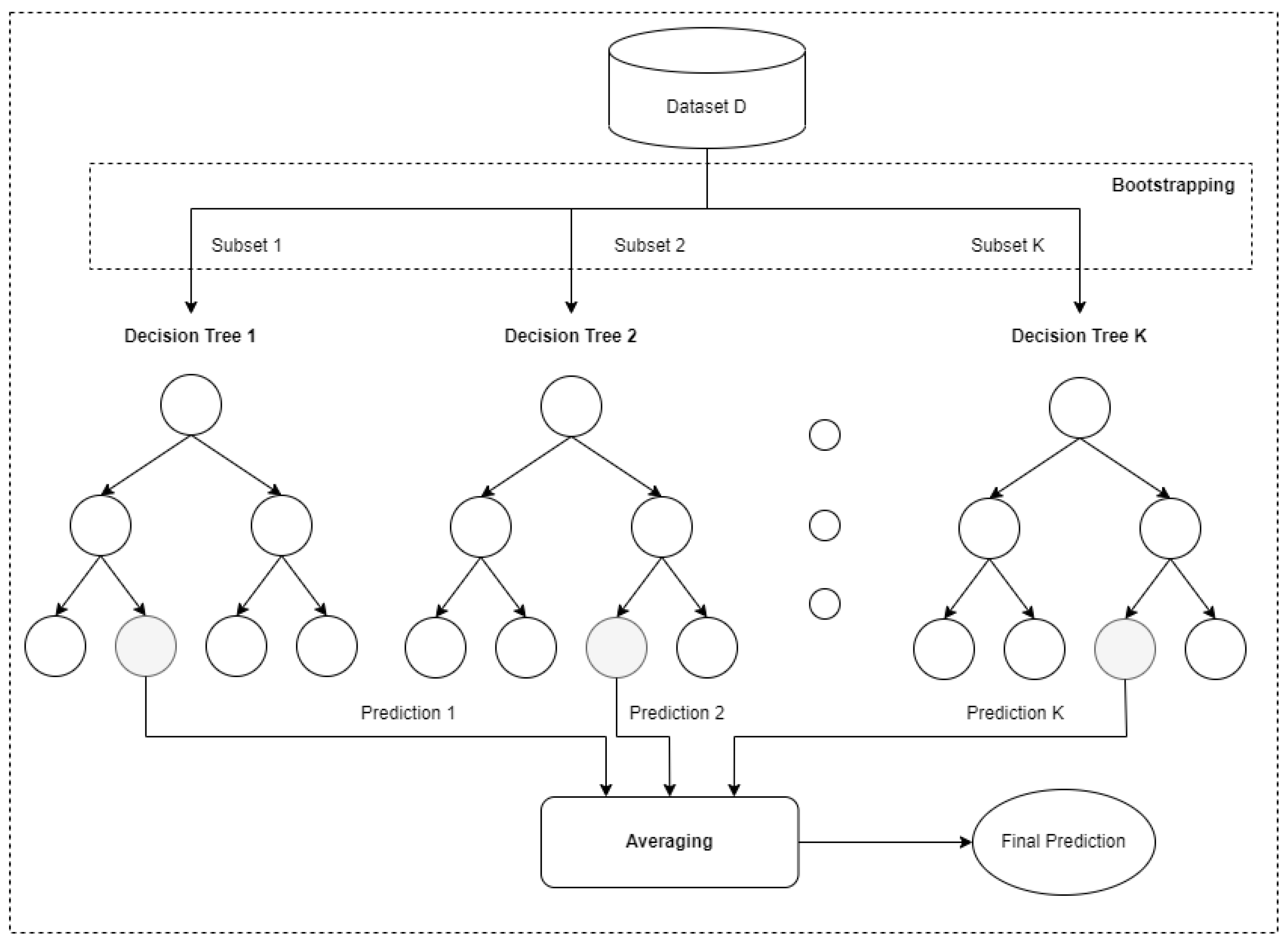
The structure of the RF algorithm for a regression task is presented in
Figure 1. More specifically, given a data set
D including
N samples, each composed of
F features, the algorithm trains a number of
K decision trees with the following process. The RF algorithm forms
K subsets of samples from the original data set
D and uses them to fit
K decision trees. Typically, each subset consists of
features (randomly selected from the original set of features) and
N samples (randomly drawn from the original data set with replacement). Note that, according to the bootstrapping process, some of the original samples may not be selected at all in any of the constructed subsets, while others may be selected multiple times. The main reason for using bootstrapping is the reduction of variance among the predictions of the trees and the mitigation of the negative effect that outliers and particular features may have in the training process.
RF models have many advantages that have led to their extensive use for a wide variety of tasks. First, it has been shown that RF regression models are very accurate when it comes to features with non-linear relationships and noisy data sets [
40,
41]. Moreover, being a tree-based method, RF models typically require little or even no data pre-processing (e.g., normalization or standardization). However, according to [
42], a major drawback of these models is the lack of interpretability. Despite the fact that RF offers better predictive accuracy in comparison to single decision trees, they sacrifice the inherent interpretability of the latter that allows for verification that the developed model has captured realistic insights from the training data [
43]. In addition to interpretability issues, the RF algorithm also involves more parameters than single decision trees, thus requiring more effort to be properly tuned. In this study, the Scikit-learn (Sklearn) implementation of the RF algorithm has been used [
44]. The most important parameters that have been fine-tuned are the following:
Number of estimators: Number of decision trees used to provide the individual predictions.
Maximum depth: Maximum possible depth for each decision tree. A deeper tree has the capacity to fit more complicated functions, but overly deep trees may result in overfitting.
Maximum features: Maximum size of the random subsets of features that the decision tree takes into consideration for determining a split to a node of the tree.
Bootstrap: A Boolean parameter that controls whether the model will apply bootstrapping or not.
3.2. Extreme Gradient Boosting
Gradient boosting (GB) is another type of ensemble learning algorithm used for both regression and classification tasks [
45]. The aim of GB, similar to other boosting techniques, is to construct a “strong learner” model by iteratively combining several “weak learner” models, each constructed so that the prediction error of the previous model is decreased (in each stage of the algorithm, a decision tree—regressor or classifier according to the task—is fit on the negative gradient of the loss function.) [
46]. Since the new models built are specialized in tackling the particular issues of the previous ones, the overall performance of the final model is effectively improved. Once all individual trees have been added to the ensemble, the final model is used to predict new samples.
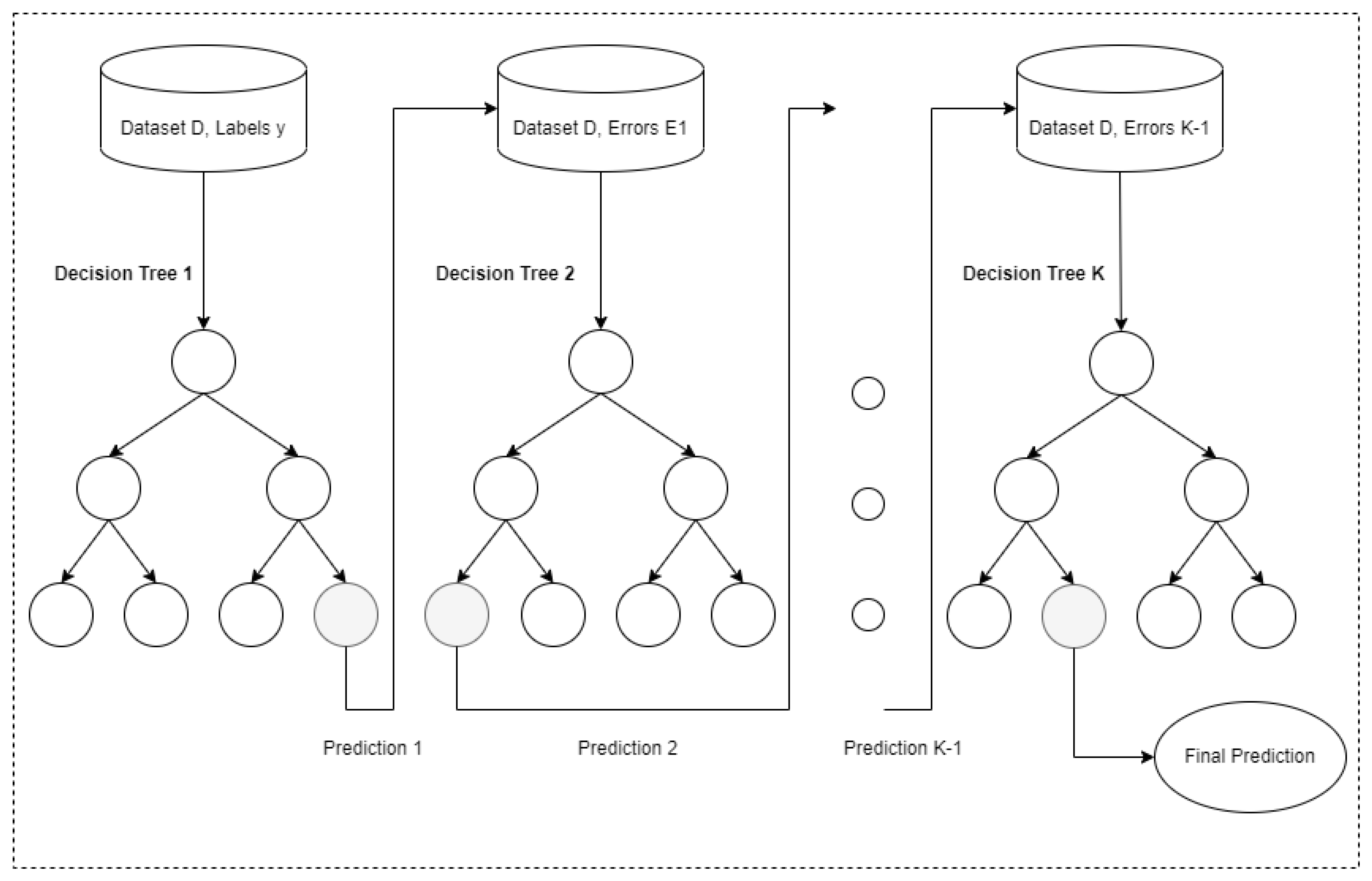
The overall architecture of the GB algorithm is presented in
Figure 2. The GB ensemble model is composed of
K decision trees. The first decision tree is trained using the input feature matrix
X and the original label
y. After the predictions of the tree have been generated, the residual errors
are calculated. The second decision tree is then trained using the
errors as labels instead of the original
y ones. The next trees are trained following the same process in an iterative fashion. Finally, when the last individual tree is trained, the training process terminates, and the complete set of trees is used for making future predictions.
In this context, XGBoost belongs to the family of GB methods but differs from them in the sense that it uses advanced regularization, namely
and
values, to enhance the generalization capabilities of the developed models. XGBoost is based on an efficient implementation of the GB algorithm, delivering higher computational performance in comparison to traditional GB models and offering reduced training times through parallelization across clusters [
47]. Note that XGBoost, like RF, also constructs ensembles from decision tree models; the main difference is that in XGBoost, the trees are added sequentially to the ensemble model and fitted in an attempt to minimize the prediction errors of the previous models (this is also the main difference between bagging and boosting). Finally, the name “gradient boosting” is due to the gradient descent optimization algorithm used to minimize the error.
XGBoost has several advantages that have established it as one of the most sovereign models for GB. As mentioned in the previous paragraph, it has a customized way of pruning the decision trees that form the ensemble, resulting in faster training and better ability to process high volume data sets [
48]. Among its optimizations, XGBoost uses an approximate greedy algorithm of weighted quantiles during the process of splitting the nodes of the trees instead of comparing all different possible splits. XGBoost also divides data to smaller segments to enable parallel processing of samples [
49], while it exploits the cache memory to save gradients and enable faster calculations [
50]. The above-mentioned features have led to its wide adoption during the last decade for classification and regression tasks in many applications.
Similar to the case of RF, XGBoost is also based on a set of hyper-parameters that are crucial for achieving high-accuracy predictions. These hyper-parameters are related not only to the GB process, including elements such as the number of trees that should be used during training, but also to the structure of each individual tree and adjusting parameters, such as the depth of the tree and the minimum loss reduction required to make a further partition on a leaf node of the tree. For the purpose of this study, the original library of the XGBoost implementation has been exploited [
47]. The most important parameters that have been fine-tuned are the following:
Number of estimators: Number of estimators (weak learners) that will be trained incrementally. A larger number of trees often results in better accuracy but may lead to overfitting, also increasing training time.
Maximum depth: Longest possible path from a root to a leaf. In general, it has been shown that the larger the tree depth, the higher the probability of over-fitting, same as in the RF algorithm.
Learning rate: This parameter is multiplied by the weight of each tree, controlling the degree the weights are updated. Lower learning rates result in smaller updates and, therefore, slower and more detailed training. On the other hand, high values may lead to divergent behavior in the loss function.
Complexity control: This parameter, also referred to as a Lagrangian multiplier, is a regularization parameter that takes values between 0 and infinity. The higher its value, the higher the regularization degree.
3.3. Light Gradient Boosting Machine
LightGBM [
51] is another GB framework, similar to XGBoost in the sense that it is based on the GB algorithm and uses decision trees as weak learners. LightGBM was originally implemented by Microsoft, focusing on performance, scalability, and optimal memory usage, and it has been widely exploited for ranking, classification, and regression ML tasks [
52].
Although LightGBM is similar to XGBoost in terms of supporting parallel processing capabilities, similar loss functions, and regularization parameters, it differs significantly in the way that decision trees are constructed. Most GB algorithms perform a depth-wise growth of the decision trees that are developed. On the contrary, LightGBM has adopted a leaf-wise method for growing the trees, selecting the leaf that has the best possible loss decrease regardless of its level of depth [
53]. This method usually results in lower loss managing to better fit to the training data. Another structural difference between the two frameworks is that LightGBM uses a different method for determining the optimal split point of the decision trees [
54]. Most GB algorithms, including XGBoost, search the optimal split point on the sorted feature values. However, LightGBM uses a histogram-based learning algorithm, which is more efficient and demands less memory.
The efficiency of LightGBM is mainly due to the use of two state-of-the-art techniques, namely gradient-based one-side sampling and exclusive feature bundling, which are combined together to form an powerful model training framework with increased accuracy compared to most GB algorithms. On the one hand, gradient-based one-side sampling is a sampling technique that is used to select samples based on their gradients. This technique aims to exploit the fact that instances with smaller gradient are better trained compared to instances with larger gradients that are considered under-trained. Thus, sampling instances with larger gradients are highly beneficial to quicker information gain. On the other hand, according to [
51], exclusive feature bundling is a novel technique that aims to reduce the number of features by regrouping mutually exclusive features into bundles, treating them as a single feature. This technique has been proven particularly effective when the feature space is sparse and several features are almost exclusive, i.e., they are usually zero at the same time. A clear example of such feature spaces are tasks that involve many categorical variables that are transformed through one-hot encoding.
The most important features that have been considered for fine-tuning the LightGBM model, implemented using the official LightGBM library for Python [
51], are the following:
Number of estimators: Number of boosted decision trees fit during the training process.
Maximum depth: Similar to RF and XGBoost, this hyper-parameter is used to limit the depth of the grown decision tree. Because of LightGBM’s lead-wise structure, fine-tuning this parameter is critical to avoid overfitting.
Number of leaves: This hyper-parameter affects the complexity of the tree model. When the number of leaves is set to , then the tree has the same number of leaves as a depth-wise tree, which is highly discouraged. On the other hand, if the number of leaves is not restricted, the model is prone to overfitting.
Learning Rate: Similar to XGBoost, this hyper-parameter affects the learning rate of the boosting process.
4. Case Study
This section is dedicated to demonstrating the experimental application of the proposed methodological framework, specifically its ability to assess the energy savings achieved by a set of real-life renovation projects. To this end, the dataset utilized in the experiment is described in detail, followed by an introduction to the experimental setup and accuracy measures employed. The results of the application are then presented, along with insightful observations gleaned from the data.
4.1. Data Set
The case study of the proposed methodology has been performed using EE investment data from various sources, such as the De-risking Energy Efficiency Platform (DEEP) database. DEEP is an open, online database including insights for many EE investment projects aspiring to enhance performance monitoring and benchmarking. Through such indicators and statistics, these databases offer stakeholders the opportunity to better understand the real benefits and risks of EE investments though market evidence and track records of thousands of EE projects from both buildings and the industry. The available data include the type and category of the EE project, the country and sector on which the project has been applied (building or industry), the projected (a priori) net annual savings, the cost of the investment, as well as several financial indicators such as the payback period, the internal rate of return, and the net present value of the investment. Moreover, the fact that the data used are open and follow the FAIR (findable, accessible, interoperable, and reusable) principles provides many benefits to the scientific community, including increased transparency, reproducibility, and collaboration, ultimately leading to better solutions to complex problems [
55].
The selection of the most suitable features for predicting the energy savings of EE renovation projects was based on previous studies [
16,
56,
57] but also performed with respect to the available data. Therefore, the selected input features are the following:
Project sector, namely whether the investment refers to a building or the industry.
Investment cost, measured in Euros.
Projected net annual savings, measured in Euros, as estimated at the time the investment was made.
Country where the EE project was applied.
Investment category, indicating the main target of the EE renovation project in terms of energy usage or building fabric (e.g., heating, cooling, lighting, pumps, or building fabric).
Investment type, indicating the nature of the EE renovation project in more detail compared to the investment category (e.g., technical versus operational optimization when it comes to pump or lighting optimization).
The data set consists of a fully anonymized sample of 4183 EE investments from 9 countries (Belgium, Bulgaria, Denmark, France, Germany, Latvia, Sweden, the United Kingdom, and the United States). This set of investments has been carefully selected, excluding EE projects with missing data in one or multiple features. From the total number of 4183 EE projects with available data, 412 projects have been ruled out as outliers, and the remaining 3771 form the final data set. The existence of outliers was pointed out by the use of distribution box plots, and the method followed to identify potential outliers in this specific dataset is based on the extraction of the top and bottom percentiles using the ratio of cost to energy savings. More specifically, any data point that falls outside of the range defined by the 5th and 95th percentiles of the datasets have been considered as outliers, in order to rule out unrealistic records subject to human error in the process of collecting the information. The most demanding pre-processing step, though, has been the formulation of investment categories and investment types in a mutually exclusive and collectively exhaustive way. As seen in
Table 1, there are a total of 8 EE investment categories, consisting of 27 discrete investment types.
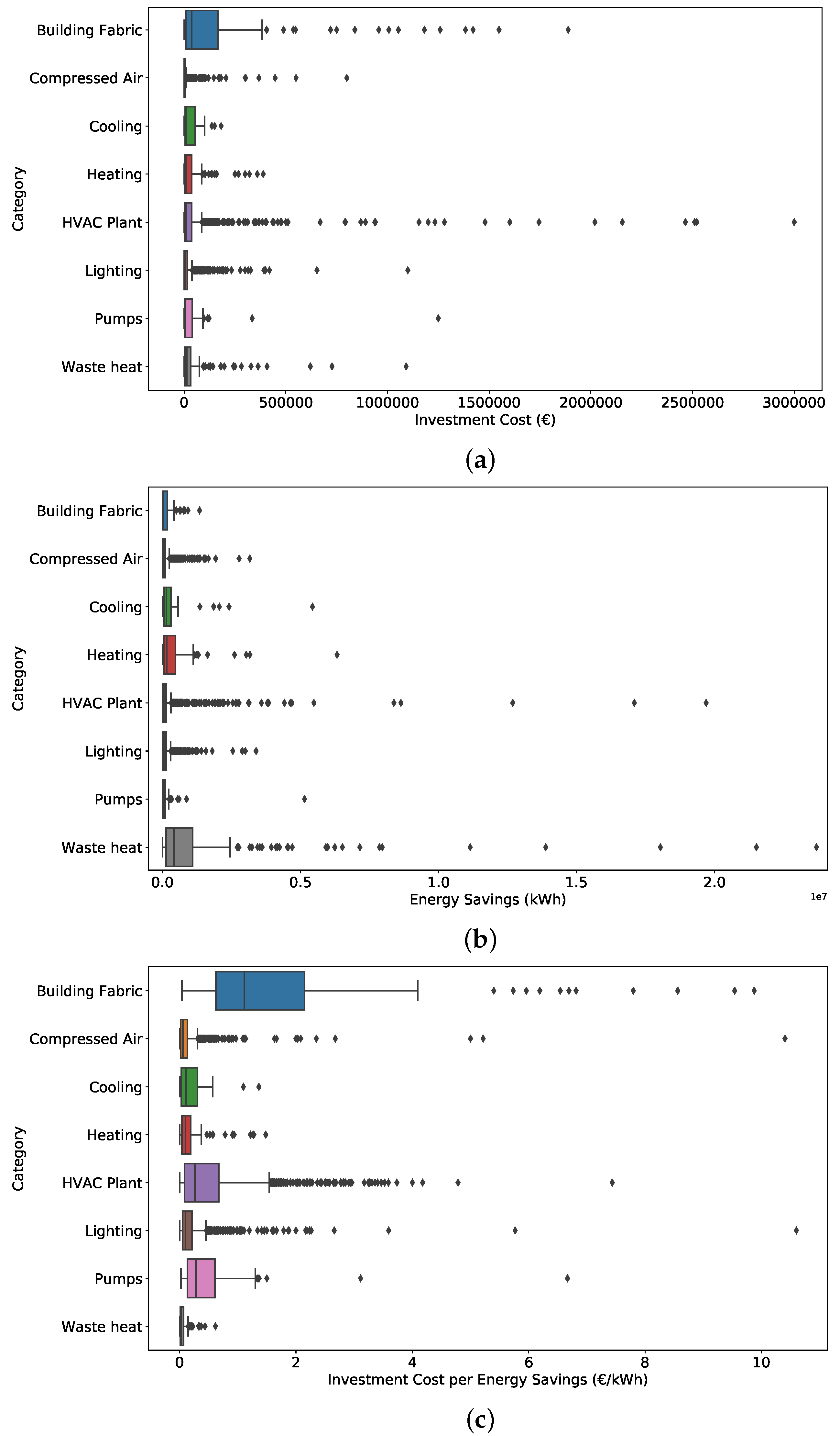
Given the inherent structural and technical differences of each type of investment, a high degree of variability is expected among the considered categories (or even types of of investment), both in terms of investment cost and energy savings achieved by the respective EE actions. A representative visualization of these differences among the investment categories is presented in
Figure 3. The box plots of
Figure 3 provide a summary of each feature, including the minimum score, first quartile, median, third quartile, and maximum score. It should be noted that the individual points that are located outside the whiskers of the box plot are possible outliers (an observation that is numerically distant from the rest of the data). In
Figure 3a, we observe that the most costly investment categories are the building fabric measures and the HVAC plant, while on the other hand the heating, lighting, and compressed air actions can be considered among the least expensive ones. In terms of energy savings, it is observed that building fabric measures are among the lowest performing categories despite the high investment cost they involve. On the contrary, waste heat actions bring on significant energy savings, as seen in
Figure 3b. Finally, in
Figure 3c, we present the index of investment efficiency defined as the ratio of investment cost per energy savings (EUR/kWh). Effectively, this index indicates which categories are more effective in the sense that they result in great energy savings when compared to the corresponding cost of investment. According to this index, and as expected from our previous observations, building fabric measures is the least efficient category, while several investments in HVAC plants, lighting, and pumps have also low efficiency. On the other hand, compressed air, heating, and waste heat investments can be ranked among the most effective categories of measures.
4.2. Experimental Setup
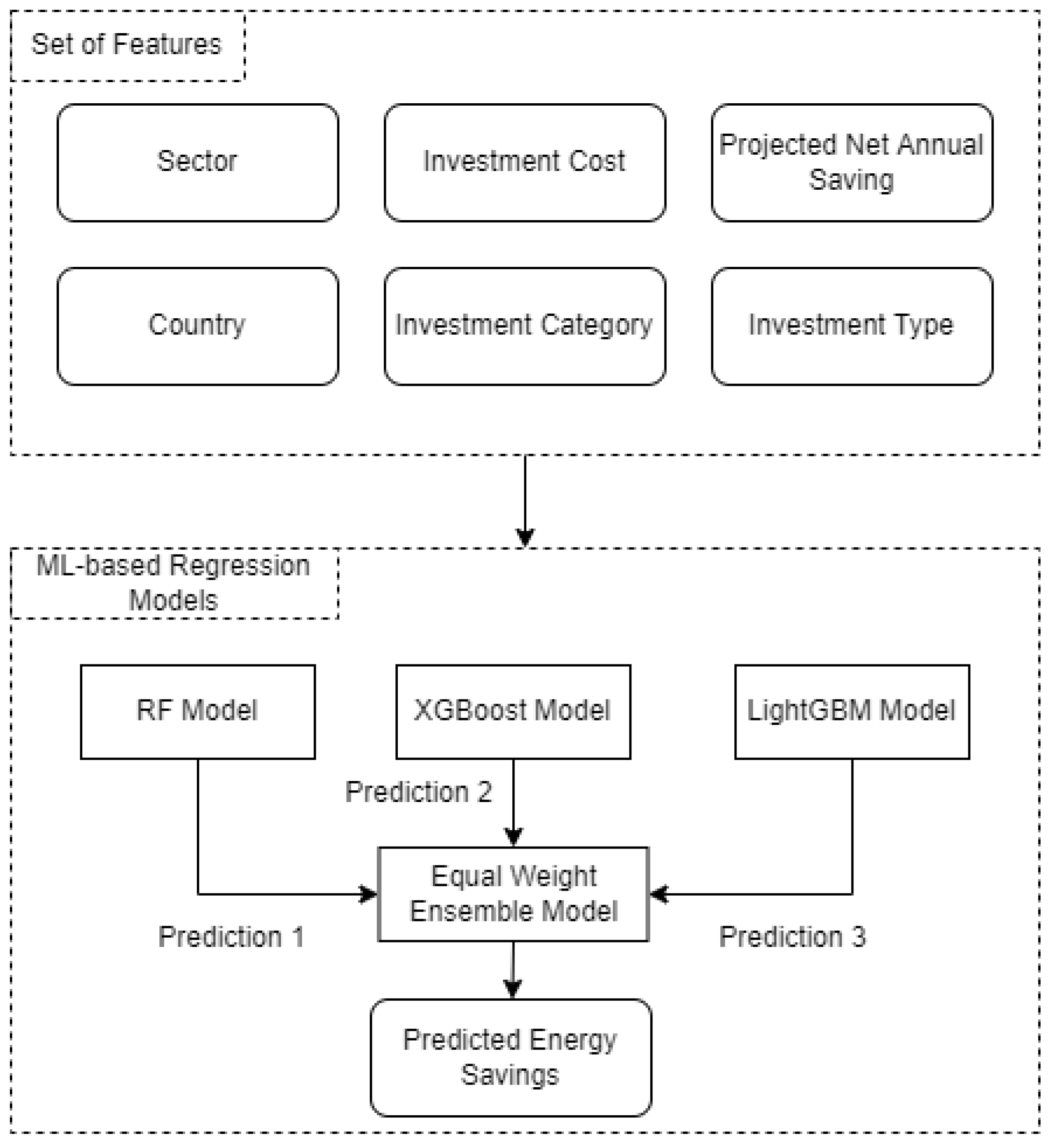
In this subsection, we present the setup of the experimental application regarding the evaluation of the proposed ML-based framework for estimating energy savings of EE renovation actions. The structure of the experimental application is summarized in
Figure 4. As can be seen, the input of the methodology consists of the six features presented in
Section 4.1. Some of these features are used without being further processed. However, the categorical variables, namely the sector, country, investment category, and investment type, have been categorically encoded with the label encoder function. For example, for the sector feature, the category “Building” has been encoded with the value of 0, while the category “Industry” has the value of 1. Following this, the final data set is split into training and test sets with random sampling, keeping 80% of the data set for the training, and the remaining 20% for the evaluation of the proposed framework.
The core of the ML framework proposed in this study involve the tree-based algorithms presented in
Section 3. These algorithms are based on decision trees and exploit some of the most successful ensembling techniques like bagging and boosting. Thus, we have employed the RF, the XGBoost, and the LightGBM models to predict the energy savings of EE renovation actions. Moreover, we have applied an extra ensembling level in order to blend the predictions of the three tree-based models with the objective to mitigate model and parameter uncertainty [
58]. In this respect, after the three models generate their predictions, their values are averaged using equal weights to obtain the final forecast, i.e., energy savings for the examined EE renovation actions. Effectively, this extra level of ensembling reduces the spread or dispersion of the predictions and further improves forecasting performance (for an encyclopedic review on the benefits of ensembling in forecasting, please refer to section 2.6 of [
55]).
The final step of the experimental setup involves the determination of the hyper-parameters for the selected regression models. For each of the models, the optimal hyper-parameter values were determined using part (20%) of the data available for training as a validation set. In order to make sure that the ML models will be robust for all investment categories, the validation set consisted of samples that represented different categories, measures, and countries of the original data set. The mean absolute and squared errors were used to identify the optimal hyper-parameter values for each model. The optimization of the hyper-parameter values was conducted using grid search. The results of the hyper-parameter fine-tuning process for each model are summarized in
Table 2 along with the respective search space and selected values.
4.3. Accuracy Measures
The selection of the most appropriate accuracy measures is a necessary step for the evaluation of any regression model. In this study, we evaluate the accuracy of the four models (the three models presented in
Section 3 and the ensemble model) based on the mean absolute error (
MAE), the mean absolute percentage error (
MAPE), the root mean squared error (
RMSE), and the coefficient of determination (
) between the forecasts and the real values [
59].
MAE is the average of all absolute errors between the real and the predicted value, thus being relatively robust to outliers and easy to interpret, as it is expressed at the same scale as the actual observations. On the other hand,
RMSE gives a relatively higher weight to larger errors and therefore helps in the detection of large mispredictions by the models. Both measures are very useful for the interpretation of the results, but when it comes to comparing different investment categories (which have different scales of energy savings), the use of scale-independent measures is necessary.
MAPE is such a measure that incorporates scale-independence and high interpretability. Moreover, since the data set does not include any zero values that affect the ability to calculate
MAPE, this measure is highly beneficial for comparing the accuracy of the models on different investment categories. Finally,
is a statistical measure that shows the proportion of variance the predictions explain over the target variable, being an indicator of how well the data fit the regression models. The formulas for computing the above-mentioned measures are presented as follows:
where
y and
are the real and the predicted value of the energy savings for the examined EE investment in the test set, respectively,
is the average value of the real observations, and
n is the total number of the samples included in the evaluation.
4.4. Results and Discussion
The proposed ML methodology has been evaluated on a test set consisting of 754 EE investments, i.e., 20% of the whole data set. The test set includes samples from all the investment categories considered in order to evaluate the robustness of the models in different types of EE projects. The results of the experimental application are presented in
Table 3. Our results indicate that all three tree-based models can effectively take into account the inherent difficulties of such a complex prediction task as the problem of estimating the energy savings of various renovation actions of different categories applied in different countries. Among the three tree-based models, XGBoost performs best in terms of
MAE (25,613 kWh) and
MAPE (32.6%), while LightGBM and RF achieve a slightly higher
score of 78.7%. On the other hand, although RF has the highest
MAE and
MAPE error scores among the three models, it is better in terms of
RMSE (50,459 kWh), indicating that the RF model has less significant errors compared to the other models.
Our results indicate that models based on boosting (XGBoost and LightGBM) are generally better in terms of measures that do not penalize large errors, while RF, which based on bagging, performs better in measures like RMSE that highly value large mispredictions. In this context, the proposed equal weight (EW) ensemble model outperforms all three models in all error indexes. More specifically, the EW ensemble model achieves an RMSE index of 49,806 kWh, an MAE index of 25,339 kWh, an MAPE index of 32.2%, and an score of 79.2%. These results confirm that the proposed ensembling model has higher predictive accuracy compared to the individual models, managing to improve the generalization error of the individual tree-based models it builds on.
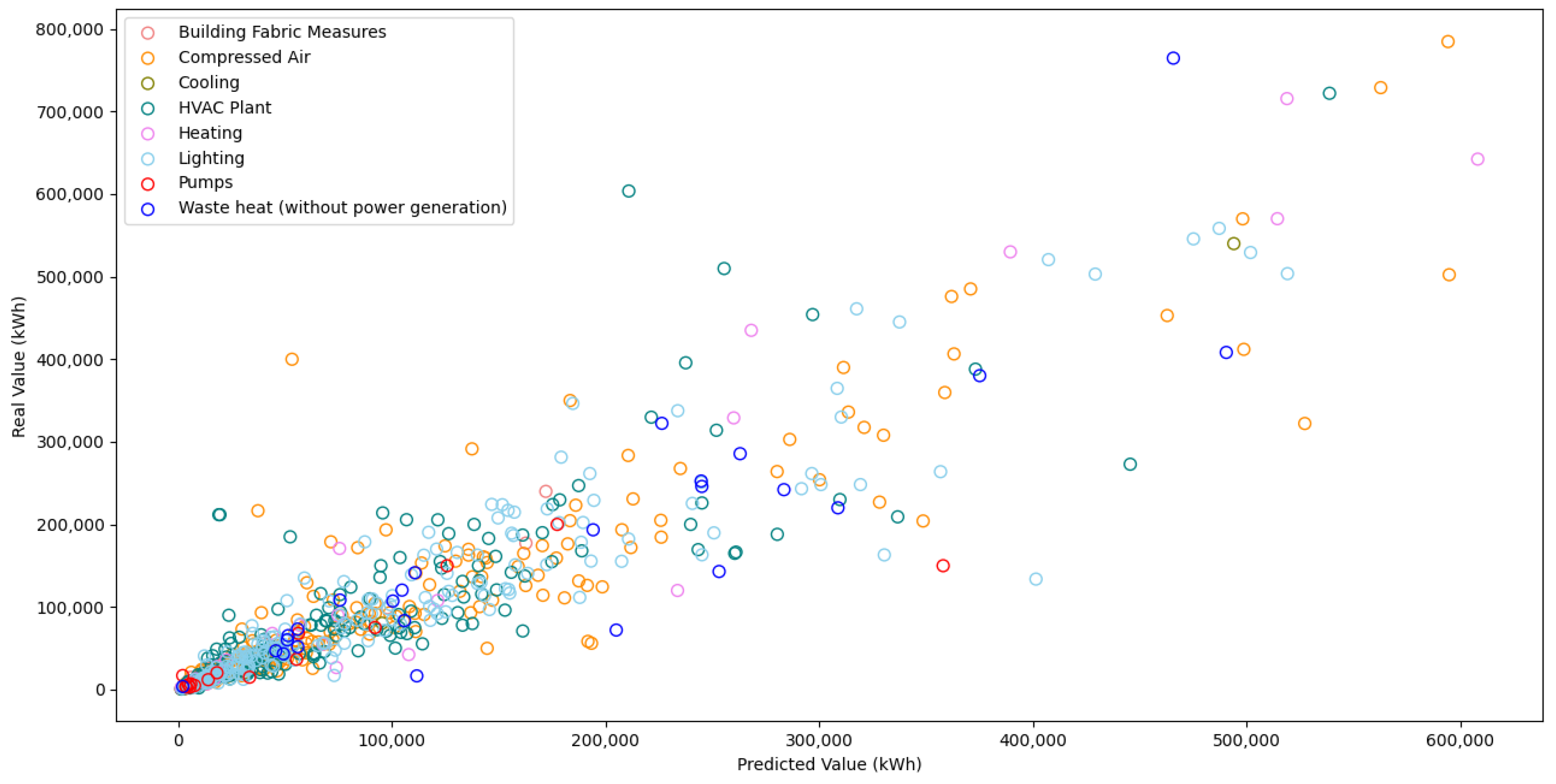
Finally, a very significant aspect of the empirical evaluation is to measure the predictive ability of the ensemble model in different investment categories. A scatter plot of the real values against the predicted values for the EW ensemble model is shown in
Figure 5, where different colors are used to indicate the category of each EE project. As one may assume, some renovation categories (e.g., lighting) are expected to be easier to predict in general, while others (e.g., heating) are more demanding due to the inherent variability of the energy consumption, a fact that is visually confirmed by
Figure 5 (the farther the dots are placed from the diagonal of the scatter plot, the larger the prediction error is). In this respect,
Table 4 presents the
MAPE and
measures of the EW ensemble model per investment category. These measures have been selected for comparing different categories because they are scale-independent, contrary to
RMSE and
MAE that are not suitable for evaluating accuracy across groups of data with different scales. We find that the ensemble model performs relatively better for the cooling, lighting, and compressed air categories, producing less accurate results for the waste heat and pumps categories. This can be attributed to the nature of the former types of measures, incorporating a low degree of variability regarding the achieved energy savings.
5. Conclusions
In this study, we proposed an ML-based framework for predicting the energy savings of various types of EE renovations. The basis of our framework consists of three widely-used tree-based ensembling algorithms, namely RF, XGBoost, and LightGBM. The single predictions generated by the tree-based models are then blended using another level of ensembling that applies equal weights to further mitigate prediction uncertainty and improve forecasting performance.
The predictive accuracy of the base models and their ensemble has been empirically evaluated through an experimental application using a database of EE renovation investments. Our results indicate that, according to four accuracy measures considered, the ensemble model can generate more accurate forecasts than the three individual ML models. Moreover, we find that some types of EE measures may be easier to predict than others, an insight that can be exploited by stakeholders when estimating the risk of their investments. Nevertheless, no EE categories with extremely bad predictions were identified.
This study forms a basis towards accurately estimating the potential savings of EE renovations. However, there is definitely much space for improvement. Firstly, future research can combine physical modeling and data-driven modeling techniques to overcome the limitations of each approach, taking advantage of the strengths of both to develop more accurate and comprehensive methods for estimating energy savings. Another very promising direction of future research is the organization of a structured process to collect and verify data regarding EE measures. This could result in a uniform, open database, including a significantly larger number of EE renovations, as well as more types and categories of actions applied in a more diverse set of countries with different climate characteristics. Such a collection process would also enable the acquisition of a more detailed set of features for each project, including but not limited to information that refers to the floor area, year of construction, occupancy, operating hours, and type of building, which could contribute to improved forecasting performance. Finally, given that no prediction can be perfect, future work could try to link forecast error with the potential uncertainty of EE investments to support decisions in EE financing. Moving one step further, the development of a predictions-as-a-service, web-based tool incorporating the above-mentioned enhancements would definitely add value in the decision making process of various stakeholders in the field of EE financing.
Author Contributions
Conceptualization, E.S. (Elissaios Sarmas), E.S. (Evangelos Spiliotis), N.D., V.M. and H.D.; methodology, E.S. (Elissaios Sarmas), E.S. (Evangelos Spiliotis), N.D., V.M. and H.D.; software, E.S. (Elissaios Sarmas) and E.S. (Evangelos Spiliotis); validation, E.S. (Elissaios Sarmas) and E.S. (Evangelos Spiliotis); formal analysis, E.S. (Elissaios Sarmas), E.S. (Evangelos Spiliotis), N.D., V.M. and H.D.; investigation, E.S. (Elissaios Sarmas), E.S. (Evangelos Spiliotis), N.D., V.M. and H.D.; resources, V.M. and H.D.; data curation, E.S. (Elissaios Sarmas) and E.S. (Evangelos Spiliotis); writing—original draft preparation, E.S. (Elissaios Sarmas), E.S. (Evangelos Spiliotis), N.D., V.M. and H.D.; writing—review and editing, E.S. (Elissaios Sarmas), E.S. (Evangelos Spiliotis), N.D., V.M. and H.D.; visualization, E.S. (Elissaios Sarmas) and E.S. (Evangelos Spiliotis); supervision, E.S. (Evangelos Spiliotis), V.M. and H.D.; project administration, V.M. and H.D.; funding acquisition, V.M. and H.D. All authors have read and agreed to the published version of the manuscript.
Funding
The work presented is based on research conducted within the framework of the project “Modular Big Data Applications for Holistic Energy Services in Buildings (MATRYCS)”, of the European Union’s Horizon 2020 research and innovation programme under grant agreement no. 1010000158 (
https://matrycs.eu/, accessed on 20 February 2023). The content of the paper is the sole responsibility of its authors and does not necessary reflect the views of the EC.
Data Availability Statement
The data used in the present study were retrieved from the De-risking Energy Efficiency Platform (DEEP) database (
https://deep.eefig.eu/, accessed on 20 February 2023).
Conflicts of Interest
The authors declare no conflict of interest. The funders had no role in the design of the study.
Abbreviations
The following abbreviations are used in this manuscript:
| DEEP | De-risking Energy Efficiency Platform |
| EC | European Commission |
| EE | Energy efficiency |
| EW | Equal Weight |
| GB | Gradient Boosting |
| LightGBM | Light Gradient Boosting Machine |
| MAE | Mean Absolute Error |
| MAPE | Mean Absolute Percentage Error |
| ML | Machine Learning |
| M&V | Measurement & Verification |
| NNs | Neural Network |
| RF | Random Forest |
| RMSE | Root Mean Squared Error |
| XGBoost | Extreme Gradient Boosting |
References
- Hamilton, I.; Kennard, H.; Rapf, O.; Kockat, J.; Zuhaib, S.; Abergel, T.; Oppermann, M.; Otto, M.; Loran, S.; Steurer, N.; et al. Global Status Report for Buildings and Construction: Towards a Zero-Emission; United Nations Environment Programme, Efficient and Resilient Buildings and Construction Sector: Nairobi, Kenya, 2020. [Google Scholar]
- European Commission. Directive 2010/31/EU of the European Parliament and of the Council Dated May 19, 2010 about the Overall Energy Efficiency of Buildings. 2018. Available online: https://eur-lex.europa.eu/legal-content/EN/TXT/?uri=CELEX%3A02010L0031-20100708 (accessed on 20 February 2023).
- European Commission. Directive 2010/31/EU of the European Parliament and of the Council of 19 May 2010 on the Energy Performance of Buildings. 2021. Available online: https://eur-lex.europa.eu/LexUriServ/LexUriServ.do?uri=OJ:L:2010:153:0013:0035:EN:PDF (accessed on 20 February 2023).
- IEA. Tracking Buildings 2021. Available online: https://www.iea.org/reports/buildings (accessed on 20 February 2023).
- Rosenow, J.; Eyre, N. Reinventing energy efficiency for net zero. Energy Res. Soc. Sci. 2022, 90, 102602. [Google Scholar] [CrossRef]
- Sarmas, E.; Marinakis, V.; Doukas, H. A data-driven multicriteria decision making tool for assessing investments in energy efficiency. Oper. Res. 2022, 5597–5616. [Google Scholar] [CrossRef]
- Sarmas, E.; Spiliotis, E.; Marinakis, V.; Koutselis, T.; Doukas, H. A meta-learning classification model for supporting decisions on energy efficiency investments. Energy Build. 2022, 258, 111836. [Google Scholar] [CrossRef]
- He, Y.; Liao, N.; Bi, J.; Guo, L. Investment decision-making optimization of energy efficiency retrofit measures in multiple buildings under financing budgetary restraint. J. Clean. Prod. 2019, 215, 1078–1094. [Google Scholar] [CrossRef]
- Liu, Y.; Liu, T.; Ye, S.; Liu, Y. Cost-benefit analysis for Energy Efficiency Retrofit of existing buildings: A case study in China. J. Clean. Prod. 2018, 177, 493–506. [Google Scholar] [CrossRef]
- DOE, U. International Performance Measurement & Verification Protocol. Available online: https://www.nrel.gov/docs/fy02osti/31505.pdf (accessed on 20 February 2023).
- NREL. The Uniform Methods Project: Methods for Determining Energy Efficiency Savings for Specific Measures. Available online: https://www.nrel.gov/docs/fy18osti/70472.pdf (accessed on 20 February 2023).
- ASHRAE. Measurement of Energy, Demand, and Water Savings; ASHRAE Guideline; ASHRAE: Atlanta, GA, USA, 2014; Volume 4, pp. 1–150. [Google Scholar]
- Manfren, M.; Nastasi, B. Parametric performance analysis and energy model calibration workflow integration—A scalable approach for buildings. Energies 2020, 13, 621. [Google Scholar] [CrossRef] [Green Version]
- Gallagher, C.V.; Leahy, K.; O’Donovan, P.; Bruton, K.; O’Sullivan, D.T. Development and application of a machine learning supported methodology for measurement and verification (M&V) 2.0. Energy Build. 2018, 167, 8–22. [Google Scholar]
- Sarmas, E.; Dimitropoulos, N.; Marinakis, V.; Zucika, A.; Doukas, H. Monitoring the impact of energy conservation measures with Artificial Neural Networks. In Proceedings of the ECEEE 2022 Summer Study Proceedings Agents of Change (ECEEE), Online, 6–11 June 2022. [Google Scholar]
- Doukas, H.; Xidonas, P.; Mastromichalakis, N. How successful are energy efficiency investments? A comparative analysis for classification & performance prediction. Comput. Econ. 2022, 59, 579–598. [Google Scholar]
- Grillone, B.; Danov, S.; Sumper, A.; Cipriano, J.; Mor, G. A review of deterministic and data-driven methods to quantify energy efficiency savings and to predict retrofitting scenarios in buildings. Renew. Sustain. Energy Rev. 2020, 131, 110027. [Google Scholar] [CrossRef]
- Marinakis, V. Big data for energy management and energy-efficient buildings. Energies 2020, 13, 1555. [Google Scholar] [CrossRef] [Green Version]
- Manfren, M.; James, P.A.; Tronchin, L. Data-driven building energy modelling—An analysis of the potential for generalisation through interpretable machine learning. Renew. Sustain. Energy Rev. 2022, 167, 112686. [Google Scholar] [CrossRef]
- Chou, J.S.; Bui, D.K. Modeling heating and cooling loads by artificial intelligence for energy-efficient building design. Energy Build. 2014, 82, 437–446. [Google Scholar] [CrossRef]
- Singaravel, S.; Suykens, J.; Geyer, P. Deep-learning neural-network architectures and methods: Using component-based models in building-design energy prediction. Adv. Eng. Inform. 2018, 38, 81–90. [Google Scholar] [CrossRef]
- Al-Rakhami, M.; Gumaei, A.; Alsanad, A.; Alamri, A.; Hassan, M.M. An ensemble learning approach for accurate energy load prediction in residential buildings. IEEE Access 2019, 7, 48328–48338. [Google Scholar] [CrossRef]
- Ngo, N.T. Early predicting cooling loads for energy-efficient design in office buildings by machine learning. Energy Build. 2019, 182, 264–273. [Google Scholar] [CrossRef]
- Paterson, G.; Mumovic, D.; Das, P.; Kimpian, J. Energy use predictions with machine learning during architectural concept design. Sci. Technol. Built Environ. 2017, 23, 1036–1048. [Google Scholar] [CrossRef]
- Geyer, P.; Singaravel, S. Component-based machine learning for performance prediction in building design. Appl. Energy 2018, 228, 1439–1453. [Google Scholar] [CrossRef]
- Naji, S.; Keivani, A.; Shamshirband, S.; Alengaram, U.J.; Jumaat, M.Z.; Mansor, Z.; Lee, M. Estimating building energy consumption using extreme learning machine method. Energy 2016, 97, 506–516. [Google Scholar] [CrossRef]
- Marasco, D.E.; Kontokosta, C.E. Applications of machine learning methods to identifying and predicting building retrofit opportunities. Energy Build. 2016, 128, 431–441. [Google Scholar] [CrossRef] [Green Version]
- Severinsen, A.; Myrland, Ø. Statistical learning to estimate energy savings from retrofitting in the Norwegian food retail market. Renew. Sustain. Energy Rev. 2022, 167, 112691. [Google Scholar] [CrossRef]
- Ali, U.; Shamsi, M.H.; Bohacek, M.; Hoare, C.; Purcell, K.; Mangina, E.; O’Donnell, J. A data-driven approach to optimize urban scale energy retrofit decisions for residential buildings. Appl. Energy 2020, 267, 114861. [Google Scholar] [CrossRef]
- Geyer, P.; Schlüter, A.; Cisar, S. Application of clustering for the development of retrofit strategies for large building stocks. Adv. Eng. Inform. 2017, 31, 32–47. [Google Scholar] [CrossRef]
- Poortinga, W.; Jiang, S.; Grey, C.; Tweed, C. Impacts of energy-efficiency investments on internal conditions in low-income households. Build. Res. Inf. 2018, 46, 653–667. [Google Scholar] [CrossRef] [Green Version]
- Januschowski, T.; Wang, Y.; Torkkola, K.; Erkkilä, T.; Hasson, H.; Gasthaus, J. Forecasting with trees. Int. J. Forecast. 2021, 38, 1473–1481. [Google Scholar] [CrossRef]
- Breiman, L. Random forests. Mach. Learn. 2001, 45, 5–32. [Google Scholar] [CrossRef] [Green Version]
- Spiliotis, E. Decision Trees for Time-Series Forecasting. Foresight Int. J. Appl. Forecast. 2022, 64, 30–44. [Google Scholar]
- Geurts, P.; Ernst, D.; Wehenkel, L. Extremely randomized trees. Mach. Learn. 2006, 63, 3–42. [Google Scholar] [CrossRef] [Green Version]
- Sagi, O.; Rokach, L. Ensemble learning: A survey. Wiley Interdiscip. Rev. Data Min. Knowl. Discov. 2018, 8, e1249. [Google Scholar] [CrossRef]
- Breiman, L. Bagging predictors. Mach. Learn. 1996, 24, 123–140. [Google Scholar] [CrossRef] [Green Version]
- Prasad, A.M.; Iverson, L.R.; Liaw, A. Newer classification and regression tree techniques: Bagging and random forests for ecological prediction. Ecosystems 2006, 9, 181–199. [Google Scholar] [CrossRef]
- Strobl, C.; Malley, J.; Tutz, G. An introduction to recursive partitioning: Rationale, application, and characteristics of classification and regression trees, bagging, and random forests. Psychol. Methods 2009, 14, 323. [Google Scholar] [CrossRef] [PubMed] [Green Version]
- Cheng, L.; De Vos, J.; Zhao, P.; Yang, M.; Witlox, F. Examining non-linear built environment effects on elderly’s walking: A random forest approach. Transp. Res. Part Transp. Environ. 2020, 88, 102552. [Google Scholar] [CrossRef]
- Anifowose, F.A.; Labadin, J.; Abdulraheem, A. Ensemble model of non-linear feature selection-based extreme learning machine for improved natural gas reservoir characterization. J. Nat. Gas Sci. Eng. 2015, 26, 1561–1572. [Google Scholar] [CrossRef]
- Aria, M.; Cuccurullo, C.; Gnasso, A. A comparison among interpretative proposals for Random Forests. Mach. Learn. Appl. 2021, 6, 100094. [Google Scholar] [CrossRef]
- Freitas, A.A. Comprehensible classification models: A position paper. ACM SIGKDD Explor. Newsl. 2014, 15, 1–10. [Google Scholar] [CrossRef]
- Pedregosa, F.; Varoquaux, G.; Gramfort, A.; Michel, V.; Thirion, B.; Grisel, O.; Blondel, M.; Prettenhofer, P.; Weiss, R.; Dubourg, V.; et al. Scikit-learn: Machine Learning in Python. J. Mach. Learn. Res. 2011, 12, 2825–2830. [Google Scholar]
- Natekin, A.; Knoll, A. Gradient boosting machines, a tutorial. Front. Neurorobot. 2013, 7, 21. [Google Scholar] [CrossRef] [Green Version]
- Schapire, R.E. The boosting approach to machine learning: An overview. In Nonlinear Estimation and Classification; Springer: New York, NY, USA, 2003; pp. 149–171. [Google Scholar]
- Chen, T.; Guestrin, C. XGBoost: A Scalable Tree Boosting System. In Proceedings of the 22nd ACM SIGKDD International Conference on Knowledge Discovery and Data Mining, KDD ’16, San Francisco, CA, USA, 13–17 August 2016; ACM: New York, NY, USA, 2016; pp. 785–794. [Google Scholar] [CrossRef] [Green Version]
- Wade, C. Hands-On Gradient Boosting with XGBoost and Scikit-Learn: Perform Accessible Machine Learning and Extreme Gradient Boosting with Python; Packt Publishing Ltd.: Birmingham, UK, 2020. [Google Scholar]
- Wen, Z.; Shi, J.; He, B.; Chen, J.; Ramamohanarao, K.; Li, Q. Exploiting GPUs for efficient gradient boosting decision tree training. IEEE Trans. Parallel Distrib. Syst. 2019, 30, 2706–2717. [Google Scholar] [CrossRef]
- Mitchell, R.; Frank, E. Accelerating the XGBoost algorithm using GPU computing. PeerJ Comput. Sci. 2017, 3, e127. [Google Scholar] [CrossRef] [Green Version]
- Ke, G.; Meng, Q.; Finley, T.; Wang, T.; Chen, W.; Ma, W.; Ye, Q.; Liu, T.Y. Lightgbm: A highly efficient gradient boosting decision tree. In Proceedings of the Advances in Neural Information Processing Systems 30 (NIPS 2017), Long Beach, CA, USA, 4–9 December 2017; Volume 30. [Google Scholar]
- Makridakis, S.; Spiliotis, E.; Assimakopoulos, V. M5 accuracy competition: Results, findings, and conclusions. Int. J. Forecast. 2022, 38, 1346–1364. [Google Scholar] [CrossRef]
- Jin, D.; Lu, Y.; Qin, J.; Cheng, Z.; Mao, Z. SwiftIDS: Real-time intrusion detection system based on LightGBM and parallel intrusion detection mechanism. Comput. Secur. 2020, 97, 101984. [Google Scholar] [CrossRef]
- Al Daoud, E. Comparison between XGBoost, LightGBM and CatBoost using a home credit dataset. Int. J. Comput. Inf. Eng. 2019, 13, 6–10. [Google Scholar]
- Petropoulos, F.; Apiletti, D.; Assimakopoulos, V.; Babai, M.Z.; Barrow, D.K.; Ben Taieb, S.; Bergmeir, C.; Bessa, R.J.; Bijak, J.; Boylan, J.E.; et al. Forecasting: Theory and practice. Int. J. Forecast. 2022, 38, 705–871. [Google Scholar] [CrossRef]
- Isa, M.; Rahman, M.M.G.M.A.; Sipan, I.; Hwa, T.K. Factors affecting green office building investment in Malaysia. Procedia-Soc. Behav. Sci. 2013, 105, 138–148. [Google Scholar] [CrossRef] [Green Version]
- Aguirre, M.; Ibikunle, G. Determinants of renewable energy growth: A global sample analysis. Energy Policy 2014, 69, 374–384. [Google Scholar] [CrossRef] [Green Version]
- Petropoulos, F.; Hyndman, R.J.; Bergmeir, C. Exploring the sources of uncertainty: Why does bagging for time series forecasting work? Eur. J. Oper. Res. 2018, 268, 545–554. [Google Scholar] [CrossRef]
- Koutsandreas, D.; Spiliotis, E.; Petropoulos, F.; Assimakopoulos, V. On the selection of forecasting accuracy measures. J. Oper. Res. Soc. 2022, 73, 937–954. [Google Scholar] [CrossRef]
| Disclaimer/Publisher’s Note: The statements, opinions and data contained in all publications are solely those of the individual author(s) and contributor(s) and not of MDPI and/or the editor(s). MDPI and/or the editor(s) disclaim responsibility for any injury to people or property resulting from any ideas, methods, instructions or products referred to in the content. |
© 2023 by the authors. Licensee MDPI, Basel, Switzerland. This article is an open access article distributed under the terms and conditions of the Creative Commons Attribution (CC BY) license (https://creativecommons.org/licenses/by/4.0/).


 ,
, 


