Review

A Comprehensive Review of Conventional, Machine Leaning, and Deep Learning Models for Groundwater Level (GWL) Forecasting

1
Department of Environmental & IT Engineering, Chungnam National University, Daejeon 34134, Republic of Korea
2
Department of Computer Engineering, Chungnam National University, Daejeon 34134, Republic of Korea
3
SafeTechResearch, Inc., Daejeon 34134, Republic of Korea
4
Department of Computer Science, College of Computer Science and Information Technology, Jazan University, Jazan 45142, Saudi Arabia
*
Author to whom correspondence should be addressed.
Appl. Sci. 2023, 13(4), 2743; https://doi.org/10.3390/app13042743
Submission received: 19 January 2023 / Revised: 14 February 2023 / Accepted: 17 February 2023 / Published: 20 February 2023

Abstract

:
Groundwater level (GWL) refers to the depth of the water table or the level of water below the Earth’s surface in underground formations. It is an important factor in managing and sustaining the groundwater resources that are used for drinking water, irrigation, and other purposes. Groundwater level prediction is a critical aspect of water resource management and requires accurate and efficient modelling techniques. This study reviews the most commonly used conventional numerical, machine learning, and deep learning models for predicting GWL. Significant advancements have been made in terms of prediction efficiency over the last two decades. However, while researchers have primarily focused on predicting monthly, weekly, daily, and hourly GWL, water managers and strategists require multi-year GWL simulations to take effective steps towards ensuring the sustainable supply of groundwater. In this paper, we consider a collection of state-of-the-art theories to develop and design a novel methodology and improve modelling efficiency in this field of evaluation. We examined 109 research articles published from 2008 to 2022 that investigated different modelling techniques. Finally, we concluded that machine learning and deep learning approaches are efficient for modelling GWL. Moreover, we provide possible future research directions and recommendations to enhance the accuracy of GWL prediction models and improve relevant understanding.

1. Introduction

Groundwater level (GWL) assessment is crucial to maintain groundwater resources, as one-third of the world’s water requirements are met through this resource [1]. It is used for domestic water supply and meets irrigation needs and industrial requirements in some parts of the world. Excessive and unplanned extraction leads to the depletion of this important resource and results in a severe issue globally, particularly in surface-water-shortage countries. So, in this regard, researchers have developed different models and techniques to simulate GWL. Modeling groundwater ranges from conceptual to numerical methods and artificial intelligence (AI) models. In numerical techniques, MODFLOW was extensively used until the previous decade to simulate GWL. However, its prediction accuracy was mainly dependent on the availability of extensive hydrogeological data and the physical characteristics of the aquifer [2]. To minimize the shortcomings of numerical methods, researchers have extensively employed artificial intelligence (AI) models over the last decade [3]. AI models do not require the physical properties of the aquifers in the GWL simulation, making them appealing to use. AI models include the most superficial artificial neural networks (ANNs), often called multilayer perceptrons (MLPs), with two or more hidden layers. ANNs having one hidden layer known as feed-forward neural networks (FFNNs) have been the most used model in the early days of AI-based research in hydrological studies [4]. Since the GWL time-series data are quite nonlinear and nonstationary, the capability of ANNs is confined to a limited set of variables. Therefore, the adaptive neuro-fuzzy inference system (ANFIS) was developed to analyze complex systems using a backpropagation algorithm and fuzzy logic [5]. It has been reported that AI (machine learning) models used to simulate GWL have shown better results than the traditional physical and numerical models because the latter needs comprehensive details of the physical properties associated with the aquifers to make a prediction [6].
However, classical machine learning models cannot learn long-term dependencies because they do not have the architecture to maintain prior information to make future predictions. To resolve this problem, researchers investigated recurrent neural networks, including RNS, GRUs, and LSTMs, and wavelet transform pre-processing data analysis to study the temporal dependencies between the multiscale input variables very well [6]. However, the prediction efficiency of the monthly, weekly, daily, and hourly basis simulations improved significantly. However, less improvement in prediction accuracy and work in the literature has been reported on yearly GWL simulation despite knowing that water management requires multi-year assessments to formulate long-term strategies to keep the balance between the supply and demand of the groundwater. Shahid et al. [7] proposed advanced studies for water treatment technologies and removing emerging contaminants. The water we consume in homes, commercial settings, or industry goes underground and damages the pure underground water. Wastewater treatment is also playing an essential role in water purification. A novel technology called “Reverse osmosis technology” is widely used on a massive scale for groundwater treatment [8]. Another experimental study on CO2 utilization in water treatment systems is based on the membrane for reducing the capability of ionic precipitation on the membrane surface and successive level expansion [9].
The comparison discussed in this review aims to evaluate the performance [10] of different machine learning (ML) [11,12,13,14] and deep learning models in predicting groundwater level (GWL) [15,16,17,18]. The groundwater level is an essential indicator of the availability of freshwater resources and is closely related to various hydrological and ecological processes. Therefore, accurate groundwater level prediction is crucial for sustainable water management and resource allocation. Machine learning is a branch of artificial intelligence that focuses on developing algorithms to learn patterns from data and make predictions based on that knowledge. There are various types of machine learning models, including decision trees [19,20,21], random forests [22,23,24,25], support vector machines (SVM) [26], and artificial neural networks (ANN). On the other hand, deep learning is a subset of machine learning that focuses on developing artificial neural networks with multiple hidden layers. These deep neural networks can learn complex patterns and relationships in data, making them particularly useful for tasks such as image recognition, natural language processing, and prediction modeling.
Consequently, different machine learning and deep learning models are applied to predict groundwater levels and their performance is compared. The comparison is based on various evaluation metrics, such as accuracy, precision, recall [27,28], and mean absolute error (MAE), R2 [29]. The comparison results provide insight into the strengths and weaknesses of different models and can help researchers and practitioners choose the most appropriate model for their specific application. Overall, comparing groundwater level prediction modeling using different machine learning and deep learning models provides valuable information for researchers and practitioners working in hydrology and water resources management.
In this paper, a collection of new theories for developing and designing a novel methodology and improving modeling efficiency are also considered in the appropriate field of evaluation. They examine modeling techniques used in all the reviewed studies; it was estimated that the machine learning and deep learning approaches are efficient enough for modeling GWL. The primary purpose of this paper is to focus on the following research question: how is GWL predicted? The recent research refers to the different stages of groundwater level prediction. In every step, the methods discussed in the reviewed studies are analyzed and compared based on their benefits and drawbacks. A new model is proposed in this study to simulate yearly GWL using wavelet Bidirectional-LSTM (W-Bi-LSTM).
The structure of the paper is as follows: Section 2 goes over the methodology of the research, Section 3 presents the groundwater and surface water data sources and availability. Section 4 illustrates the conventional, ML-, and deep-learning-based groundwater level prediction techniques. Section 5 briefly discusses the performance evaluation of different models and Section 6 represents the future research direction and discussion. Finally, Section 7 ends the paper with a conclusion.

2. Methodology of the Research

In the first stage of this research, a comprehensive review of GWL forecasting has been explored and analyzed. A few major scientific research databases, Web of Science, Scopus, etc., were decided to organize the research. The papers with the word “survey” or “review” in the keyword or abstract are reviewed. The majority of the papers were examined on GWL and selected to cite. The only available research papers on GWL prediction were studied and were chosen for our research. Once these research papers are analyzed, numerous studies are published every year. Osman et al. [30] surveyed 78 articles, and Tao et al. [31] surveyed 318 articles. As far as we know, no comprehensive study on GWL prediction is available using deep learning. These two review articles were published this year and are growing in popularity as more new research is published.
Data processing and the separation of training and testing are not included in the analysis. As the global climate continues to change, recent studies of the GWL model have used new kinds of data and applied different methods. For this reason, it is essential to consider the latest algorithms and methods, including deep learning algorithms and hybrid algorithms, along with the proprietary processing methods applied. After the analysis of available databases was concluded, the search equation was identified as the latest and very significant equation for GWL prediction. We explore the available databases to update the latest trends and analyses.
After examining the online searched databases, more than 731 papers suit the search strategy. A total of 182 of these papers were rejected, and 549 other papers were excluded from this review because their main objective was not GWL prediction. After studying the most relevant papers, the analysis was then conducted. Figure 1 shows the arithmetic conceptualization of GWL research using an AI-based model during 2008–2022. Several papers were chosen based on specific measures.
The main objectives of this research are
  • To discuss the conventional methodology for GWL.
  • To explore the current GWL methodologies.
  • Deep-learning-based models for GWL.
  • Machine -learning-perspectives-based groundwater modeling.
We used different searching keywords to find relevant studies: Set 1: “GWL” [32], “Ground-Water-level” [33]; and “Groundwater Level prediction” [34]; set 2: “Prediction”, “forecasting”, “Deep Learning”, “analysis”, “estimation”. We used the keyword AND between set1 and set2, and the OR operator was used between keywords in a set. Figure 2 illustrates the relevant and irrelevant papers selection process. Once read through the database, 731 papers met the search criteria. One hundred and eighty-two (182) duplicates were excluded from this analysis. After reviewing the titles and journals, 440 were excluded from the review because they did not go through the GWL criteria. After a thorough reading of these articles, 109 articles were finally analyzed.
All relevant papers were selected where the GWL, the data collection time, and the research project variables were tested. Many studies have used technological and water variables to model GWL. However, some studies have considered other factors to measure GWL, such as tree rings diameter, climatic conditions, area, change in population, duration, elevation, land use data, paved area, and so on. The research results are classified and analyzed in the next section based on the variables used for GWL modeling. Groundwater is a primary source of water for living things around the globe. Large urban areas generate enormous demands for water and food. India, Iran, and China are the main countries in the GWL study. Of the 20 countries surveyed, about half of the studies took place in India, Iran, and China. Other studies are centered on data collected from Azerbaijan, Greece, Bangladesh, Taiwan, Serbia, Slovenia, South Korea, the USA, and Canada.

3. Groundwater and Surface Water Data Sources and Availability

The modeling process in the groundwater–surface water (GW-SW) system is essential in understanding the interactions between these two water sources and how they impact each other. This process requires adjusting the hyperparameters of the system to ensure the simulations produced are reliable and accurate. However, data availability can sometimes pose a challenge in modeling, particularly in small areas or basins where data may be limited. Despite this, the use of GW and SW models has increased significantly in recent years due to the availability of a growing number of regional and global datasets. Global model products and open data, which contain a large amount of environmental information, have become easily accessible and, combined with the advancement of remote sensing data, provide a strong foundation for developing some water models. One of the advantages of these models is the ability to obtain critical structural aspects such as watershed boundaries, surface flow direction, and slope. This information can be taken from managing products of a digital elevation model (DEM) with the help of GIS spatial analysis. A MERIT DEM is a popular product in this field, it is a worldwide map with a resolution of approximately 90 m. The development took place using current spatial DEMs. Numerous error components, such as stripe noise, speckle noise, tree height bias, and absolute bias, have been removed to provide an unbiased representation of terrain elevation [35].
In conclusion, the modelling process in the GW-SW system is essential for understanding the interactions between these two water sources. Although data availability can sometimes pose a challenge, the use of GW and SW prototypes has dramatically increased in recent years due to the availability of open data and global model products, which provide a solid foundation for building water models. The processing of DEM products allows for the easy extraction of critical morphological features, such as surface flow direction, watershed boundaries, and slope, making it an indispensable tool in this field.
In any situation, a DEM with a finer resolution designed for a specific region or nation can also be obtained from light detection and ranging (LiDAR) products or by spatially interpolating point elevations. Soil properties of spatial division, such as texture (proportion of clay, sand, and silt), organic matter, porosity, bulk density, and hydraulic conductivity, can greatly affect the modeling results, particularly in the surface water (SW) component. These properties play a crucial role in determining soil quality and infiltration capacity [36]. The coherent world soil catalog provides a global distribution of soil characteristics [37]. Additionally, the World Soil Information Service (WOSIS) offers access to over 196,000 soil columns [38]. The given dataset contains information about soil that is standardized and ideal for mapping soil and the Earth’s system modeling. Hydrological modeling can be affected by the lack of climate data, so many databases have been created to offer first-class meteorological data. One of these databases is the Climate Forecast System Reanalysis (CFSR) [39], which extends global meteorological information for 36 years at a resolution of less than 1 degree, allowing for detailed historical data analysis. Furthermore, the CORDEX program under the World Climate Research Program (www.euro-cordex.net) provides a platform for the compilation of comprehensive climate data at the continental level, both for historical and future predictions. These data are commonly utilized in water modeling [40,41]. Obtaining information about subsurface elements, such as hydraulic conductivity and porosity, typically requires permeability tests, which can be both expensive and time-consuming. The other solution is the version 2.0 of Global Hydrogeology Maps (GLHYMPS) of porosity and permeability [42]. The “Copernicus Land Monitoring System” provides information about the spatial distribution and changes in land cover on a continental scale through its Corine product for Land Cover (CLC), covering the period from 1990 to 2018. In order to obtain accurate results, a multi-constraint measurement is frequently necessary. The use of appropriate data and their availability for model validation and measurement is still the crucial issue that determines the effectiveness of the model. To validate and calibrate surface models, various findings have assessed the effectiveness of the moderate resolution imaging spectroradiometer (MODIS) product with encouraging outcomes. Data related to soil water content, snow cover, Normalized Vegetation Index (NDVI), and evapotranspiration can be obtained using the AppEEARS interface [43].
In addition to these open datasets, a number of modeling products have become available over the past decade. Two of the global hydrological models that have been developed are PCR-GLOBWB v2.0 [44] and WaterGAP v2.2d [45], which aim to quantify human use of surface water and groundwater, along with storage, water flows, and resources on a global level. They also provide the capability to output the post-process, such as groundwater spatiotemporal recharge and volume of river flow. However, their main limitation is the low spatial resolution. It is important to note that while these globally available datasets can be useful, it is critical to be cautious when using them as they may contain errors and inconsistencies that can result in inaccuracies in simulations. Estimating the share of groundwater through a simulation of flood hydrographs using two different time-based rainfall distributions is presented in [46]. Table 1 shows the various datasets available for use in modeling parameters and their prediction possibilities. Table 2 shows the various datasets available for use in modeling parameters and their corresponding links.

4. Groundwater Level Prediction Techniques

Forecasting is achieved using the latest and past collected data to forecast the future. This review is focusing on the evaluation of the GWL as a regression problem, and researchers investigated different types: the SVM, ANN, DT, ANFIS, GP, hybrid, and genetic models. A novel type (O) was created by introducing new algorithms that do not fit any of the former categories. ANN [47] methods are the most frequently used technique in GWL forecasting, and the number of ANN-based studies increases every year. Figure 3 shows the groundwater prediction process.

4.1. Physically Based Numerical Method—MODFLOW

Physically based numerical models remain the best methods to study the characteristics of groundwater. This is because they require comprehensive details of the physical properties of aquifer. Among the different physically based numerical models, MODFLOW is the most used model in the literature; it models groundwater movement in three dimensions using finite differences. Until the last decade, MODFLOW was used extensively, especially when sufficient data are not available. Depending upon the problem, several approaches are designed for MODFLOW, i.e., the head-oriented approach (HOA) is used to determine the three-dimensional flow of groundwater, the velocity-oriented approach (VOA) comes in handy when computing the velocity of flowing groundwater [48]. However, certain steps are needed to formulate such a model, i.e., grid design, boundary setting, time steps, and hydrologic and aquifer characteristic variables selection. Shukla and Singh [49] calibrated MODFLOW in Uttar Pradesh, India to simulate groundwater levels. Data mostly comprising of water levels collected between 2005 and 2013 were used in the study. In addition, the impact of pumping and recharge rate on the groundwater levels was also studied, and it aimed to predict the groundwater levels for five years ahead. The results showed a declining trend in groundwater levels in the region.

4.2. Machine Learning—Artificial Neural Networks (ANN)

ANN is computational representation of a mathematical model inspired by the human brain’s biological network. Simple elements called neurons, operating in parallel, constitute ANN [50]. ANNs are used to calculate unknown functions or to make future predictions of the given time series based on historical data. The most basic ANN is a three-layer structure, with input, hidden, and output layers [51]. The structural representation of classical FFNN into the network and the desired outcome is computed by the output layer. The hidden layer nodes which are situated between the input and output layers receive a set of scaled inputs and calculate an output after applying a certain learning (activation) function [52].
A sample dataset Is used to train the ANN model. Training is a process of fine-tuning the network’s adjustable parameters (known as weights and biases) to optimize the output of the algorithm. “The Levenberg-Marquardt (LM) algorithm, the backpropagation (BP) algorithm, the Bayesian regularization (BR) algorithm, and the gradient descent with momentum and adaptive learning rate back-propagation (GDX) algorithm” are some learning algorithms that have been employed to train models in the literature. Feed-forward neural networks (FFNNs), usually known as multilayer perceptrons (MLPs), are a popular and robust type of ANN that has been widely studied in hydrological studies [53]. Figure 4 shows the different kinds of data used for prediction the GWL.
ANNs have been widely used in hydrology, hydraulics, rainfall-runoff estimation, groundwater level, and quality forecasting [54,55,56]. According to recent GWL modeling studies, it has been reported that ANN simulations have shown promising results compared to conceptual techniques. In one of the first studies, Lallahem et al. [4] used ANNs to simulate monthly groundwater (GWL) for an aquifer. Inputs included evapotranspiration, averaged temperature, precipitation, rainfall, and GWL at the previous lag of 13 piezometers and the primary objective was to anticipate GWL for a specific piezometer in northern France. The advantage of the multi-layer perceptron MLP was proven by simulation results. Krishna et al. [57] compared several types of FFNNs to simulate the monthly GWL in Andhra Pradesh urban aquifer, India. Results revealed the merit of an ANN trained with the LM algorithm as compared to BP and BR algorithms. Moreover, in the experiment, the best-performing network model parameters were used to predict the GWL in nearby wells.
Sreekanth et al. [5] developed ANFIS and FFNN with an LM algorithm to estimate GWL for India’s Maheshwaram watershed. Monthly groundwater (GWL) of 22 wells, rainfall, temperature, evaporation, and relative humidity are among the input variables. FNN outperformed ANFIS in terms of accuracy when results were compared. Kouziokas et al. [58] compared multiple FFNN networks and learning methods to simulate the daily groundwater (GWL) in a well. The study area is located in Montgomery County, Pennsylvania, USA. The best model was found to be FFNN trained using the LM learning algorithm with the humidity, precipitation, and temperature as inputs.

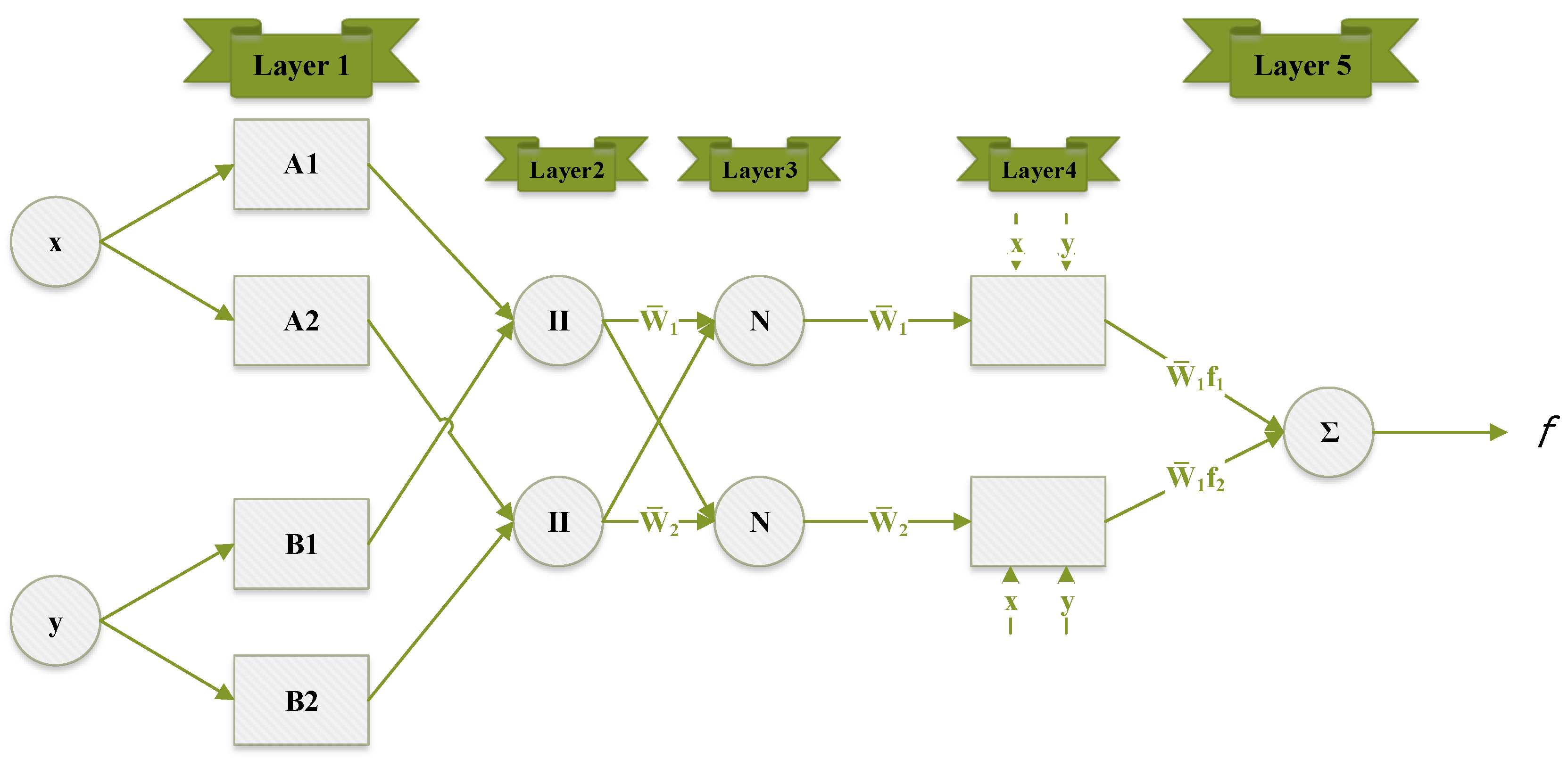
4.3. Adaptive Neuro-Fuzzy Inference System (ANFIS)

This is a hybrid technique that aims to utilize the advantage of a fuzzy inference system (FIS) with an adaptable neural network (AN). FIS is based on fuzzy logic and is good at capturing uncertainties and noise in data. Jang [59] pioneered the use of fuzzy if–then rules with right membership functions (MPs) to construct input–output pairs and a neural network learning algorithm. The fuzzy inference aystem is further classified into two approaches, namely Mamdani and Sugeno. Linear MFs are used by the Sugeno approach while Mamdani uses fuzzy MFs. ANFIS consists of five layers. The structural representation of ANFIS is similar to the ANN model, except it has two input parameters, linear and non-linear, which makes it difficult to train. Input parameters are optimized simultaneously in the training process.
Zhang et al. [60] applied three different algorithms for GWL prediction, namely, radial basis function neural network (RBFNN), ANFIS, and the grey self-memory (GSM) method. Evaluation reveals the superiority of ANFIS over the other applied algorithms based on the performance metrics result (i.e., NSE, RMSE, R2, and MARE). Bak and Bae [61] trained the ANFIS algorithm with precipitation (P) and mean temperature (Tmean) to predict GWL and reported the performance metrics RMSE as 0.1381 and MAPE as 37.869%.
Gong et al. [62] investigated the prediction accuracy of ANFIS, FNN, and SVM for monthly GWL simulation and concludes the superiority of ANFIS over other algorithms. Previous GWL, lake level, precipitation (P), and Tmean were used as input variables. Khaki et al. [63] investigated the performance of ANFIS, FFNN, and the cascade forward network (CFN) model to simulate monthly GWL at Langat Basin in Selangor state’s southeastern part. R and MSE were used as performance metrics. The ANFIS model outperformed FFNN and CFN with R = 0.94 and MSE = 0.005. Emamgholizadeh et al. [64] analyzed the differences in the monthly GWL prediction of ANN and ANFIS in Bastam plain, Iran. The following input variables were used in the study: pumping rate, rainfall recharge, and irrigation returned flow. ANFIS performed significantly better than ANN and it was also found that high accuracy can be achieved by applying different structures. Sometimes, hydrological time series data can be highly non-stationary which makes it hard for models, such as ANN and ANFIS, to better understand the underlying seasonality and thus leads to inaccurate predictions. In this situation, some researchers, such as Hsu and Li [65] and Loboda et al. [66], applied the wavelet data decomposition technique to first pre-process the input data. Wavelet transform can decompose data at various resolution levels to obtain useful information and give insights about trends and irregularities in the data. Therefore, it has several applications in hydrological studies because of the non-stationary nature of the data.
The performance of regular ANNs, ANFISs, and both coupled with the wavelet technique, i.e., WANN and WANFIS, was examined by Moosavi et al. [67]. They conducted a study to simulate monthly GWL for two subbasins in Mashad, Iran. Precipitation (P), evaporation (E), temperature (T), and previous GWL were the input variables. ANN and ANFIS failed to cope with the noise in the data while the ones coupled with wavelet performed considerably better. However, the authors reported that wavelet transform does contribute more to the efficiency of ANFIS than ANN. Another study was performed by Ebrahimi and Rajaee [68] to analyze the impact of the wavelet pre-processing technique. They developed wavelet-ANN, multi-linear regression (wavelet-MLR), and support vector machine (wavelet-SVM) up to two decomposition levels, and their regular counterparts. GWL at previous lag was used as the only input variable to simulate GWL with a one-month lead. The results showed that data decomposition translates into the high prediction accuracy of the models. Nevertheless, wavelet-ANN is reported as the best model. Machine learning models using prior wavelet data decomposition are good at yielding underlying trends and patterns at various levels in non-linear and non-stationary input data. Figure 5 shows the basic architecture of ANFIS model.

4.4. Genetic Programming (GP)

A general genetic algorithm (GA) was developed called genetic programming (GP) [69]. Darwinian theories of evolution are used for genetic programming and ecological choice as the GA. The author in [70] developed a GP-based model to predict the GWL changes and calculate the vagueness in the forecasting. The paper used Indian monthly rainfall data to predict the GWL. The GP model proposed by the author could successfully predict variations by using only hydrometeorological parameters for GWL, i.e., the model predicts without knowing the physical characteristics of the wells. GP has been mostly affected for feature selection work and optimization. Furthermore, because of its flexibility and intelligible tree structure it is more used in GW modeling. The author in [71] proposed GWL for the next day and prediction intervals of up to 7 days and applied SVM, GP, ANN, and ANFIS. All of these algorithms have prediction capabilities to predict GWL. There are several GWL combinations, including evapotranspiration and rainfall data, which are used as input to the prediction model, using data gathered from Republic of Korean, Hongcheon well station. After making a model, the autoregressive moving average (ARMA) model is used for comparison to validate the accuracy. The final conclusions proved that the ARMA methodology performed well compared to other ML methods, which is therefore the most effective with the GP model.

4.5. Deep Learning

Despite the significant performances of ANN and ANFIS in accurately predicting the GWL, these methods were confined by the vanishing and exploding gradient problem, thus hindering the capability of the machine learning models to make predictions for long-time series. A recurrent neural network (RNN) is a type of neural network that was introduced to solve the long-term dependency problem when dealing with large-scale data in the temporal domain. However, regular RNN cannot remember temporal information for long sequences, i.e., in the machine translation tasks, etc., and require large computational resources. To overcome the limitations of regular RNN, the long short-term memory (LSTM) model was proposed to keep the information for an arbitrary length. LSTM is mainly developed for continuous data—time-series data. Recently, it has been employed in various water level assessment studies.
Zhang et al. [6] proposed the LSTM model to simulate the fluctuations in water table levels using monthly water diversion, precipitation, evaporation, temperature, and previous water table level data spanning 14 years (2000–2013). The results achieved were dramatically high ( R 2 score, 0.789) when compared with the R 2 scores (0.004–0.495) of the traditional feed-forward neural network (FFNN or regular ANN). To select relevant predictors, the authors used a statistical technique that contributed to the model’s ability to generalize from the unseen data. The study was performed in five sub-areas of Hetao, China. GWL fluctuations data are prone to the existence of missing values because of several factors, i.e., human negligence, failure of recording equipment, etc. Gaps in data can make it difficult to grasp the hidden trends and seasonality. Therefore, this has led the missing values being reconstructed to fully interpret the data and make accurate predictions so that strategists can make plans for water resource management in the long run. Ren et al. [72] evaluated the ability of an LSTM model against a traditional gap-filling algorithm, ARIMA, to fill missing temporal observations for a 10-year-long dataset with dynamic gaps. The model was designed to reconstruct specification measurements (groundwater and river water interactions). The results revealed that LSTM is better at filling high dynamic gaps (daily, weekly, and sub-daily), while ARIMA excelled in reconstructing trends and seasonality-based gaps. In addition, the authors reported that LSTM can fill gaps for up to 2 days when spatial data from neighboring stations are used to make predictions. Table 3 presents detail research categorized by different algorithms: deep learning, GP, MODFLOW, ANFIS, and ANN.

5. Performance Evaluation

GWL modeling is mainly divided into two categories with regards to time, i.e., long-term, and short-term. Long-term forecasting is of great importance in various domains, for instance urban planning and water resource management, which require years of data to learn long-range dependencies. Short-term prediction is usually conducted to study variations in patterns and trends in the input variables related to the problem, for instance climatic conditions in the case of GWL. Since the target value of GWL modeling is a constant value, regression models are used in such studies. Different evaluation metrics have been used in the literature to measure the efficiency of proposed models. However, it is important to select appropriate performance metrics as it measures how well a model’s predictions compare against the true values. Root mean square error (RMSE), mean absolute error (MAE), relative error (RE), and coefficient of determination (R2) are the most common choices of researchers in the literature. Moreover, the peak elevation criteria (PEC), and low elevation criteria (LEC) are special performance measures to evaluate the model against critical parameters such as rainfall, groundwater, etc. in the case of GWL. However, most of the time RMSE and R2 have been used in GWL modeling studies. Table 4 shows different performance evaluation measures used by different experts for GWL prediction.

6. Future Research Direction and Discussion

We recommended the wavelet Bi-LSTM (W-Bi-LSTM) approach [85] to predict the groundwater level. There are two strategies, one is wavelet data decomposition [104,105,106,107] and the second is bi-directional long short-term memory (Bi-LSTM). Satellite-based techniques [108] can be used for groundwater monitoring by measuring changes in the Earth’s gravity field and surface deformation caused by water movement underground. Point-to-point satellite-based techniques, such as interferometric synthetic aperture radar (InSAR) and global navigation satellite system (GNSS), can be used to detect changes in ground elevation and surface displacement, which can be used to infer changes in the amount of groundwater. These techniques provide valuable information for managing groundwater resources and mitigating the impacts of groundwater depletion.

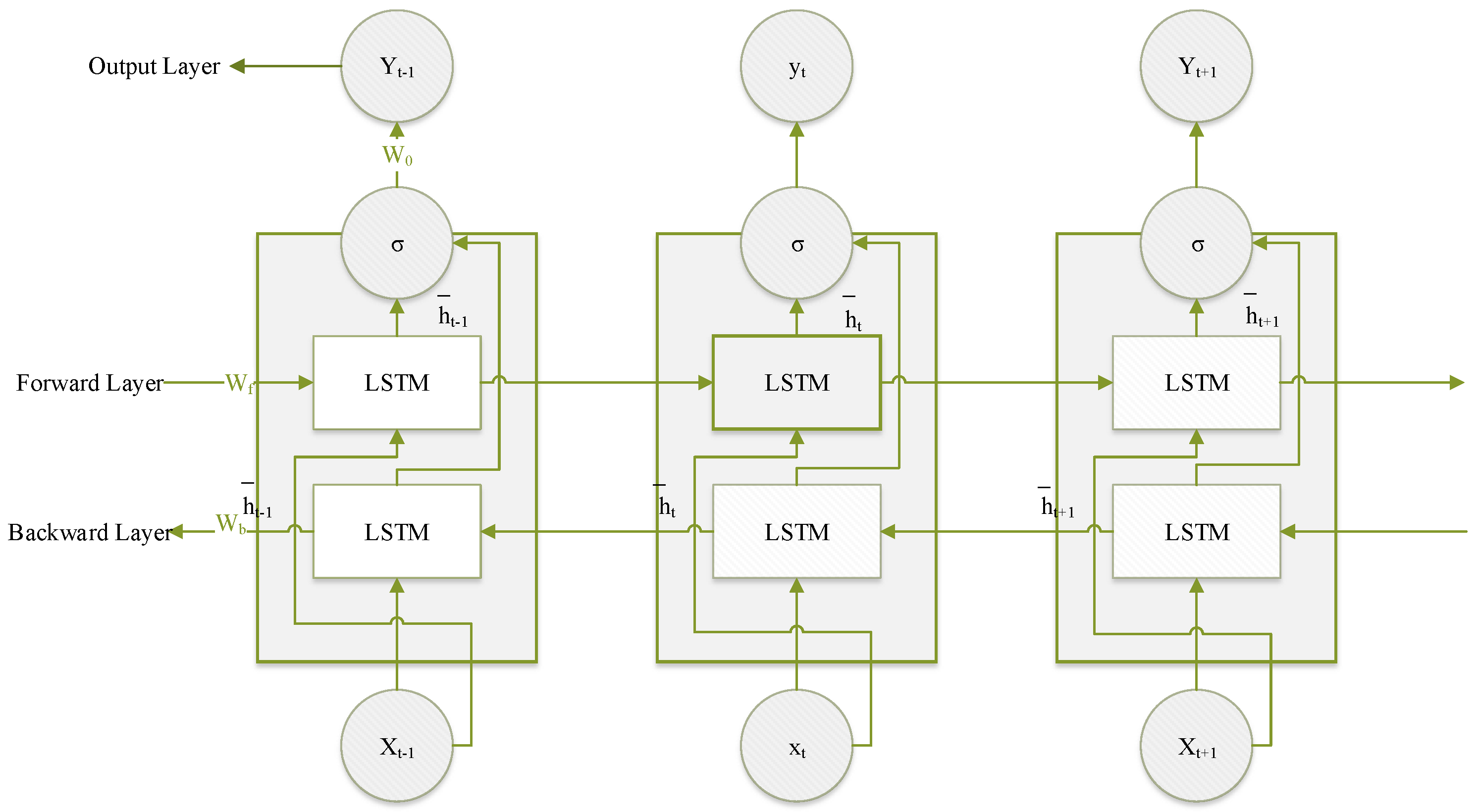
6.1. Wavelet-Bi-LSTM (W-Bi-LSTM)

As discussed above, wavelet transform (WT) is a data pre-processing tool to decompose time series in the time-frequency scale. WT is capable of decomposing the time series at various scales and into several sub-time series that give insights into the relationships between time-dependent features. To capture high-frequency information, short time intervals are used and, conversely, long-duration intervals analyze low-frequency information. Researchers report that wavelet-coupled ML models have often achieved higher prediction accuracy than regular ML models [87,88]. WT is categorized into two types: continuous wavelet transform (CWT), and discrete wavelet transform (DWT). CWT is time-consuming and computationally expensive; therefore, DWT is mostly preferred in hydrological problems, particularly in groundwater level simulation. The mathematical equation of a discrete wavelet can be represented as [89].
g ( i , j )   ( t ) = ( 1 a 0 i ) g ( ( t j b 0 a 0 i ) ( a 0 i )
In Equation (1), i and j represent the integral values, and a 0 , and b 0 are the location parameter with specified fined dilation steps and the most common values are 1 and 2, respectively. For details refer to (Cohen and Kovacevic) [90].

6.2. Wavelet-Bi-LSTM (W-Bi-LSTM)

Unlike the conventional LSTM [52], Bi-LSTM has a simultaneous two-way flow of prior information to better understand the contextual dependencies between the variables using forward hidden layers and backward hidden layers [91]. Bi-directional LSTM manages the flux of the input and output variables using several gates called memory cells, while classical recurrent neural networks (RNNs) use hidden layer nodes with nonlinear activation functions [92]. Figure 6 shows the graphical representation of Bi-LSTM. hf and hb are two memory cells in the Bi-LSTM network which manage the forward and backward computed values.
h f t = f ( w f 1 x t + w f 2 h t 1 )
h b t = f ( w b 1 x t + w b 2 h t + 1 )
In the above equations, hf represents the forward layer LSTM output and h b is the backward layer LSTM output. The final output value of the hidden layer is computed by combining the results of forward and backward layers [93].
o t = g ( w o 1 h f + w o 2 h b )
In Equations (2)–(4), wi is the weight coefficient matrix that is repeatedly applied at each time step. I hypothesize that using wavelet transform (WT) with Bi-LSTM (W-Bi-LSTM), groundwater levels can be simulated yearly with higher prediction efficiency. To the best of my knowledge, no such model has been proposed, given that, in the literature, most of the studies focused on monthly, weekly, and daily GWL predictions. Water managers and strategists need long-term assessments to keep a balance between the supply and demand of groundwater resources, therefore, yearly simulation of GWL is critical. W-Bi-LSTM can utilize the advantages of both wavelet transform and Bi-LSTM networks to make year ahead predictions. As discussed above, collected data (both meteorological and hydrological) are vulnerable to varying missing values and noise because of certain factors including human error and data collection sensor failure. The wavelet transform has the capability to decompose large-scale noisy data and find hidden periodic trends, which Bi-LSTM then uses to learn underlying long-term dependencies between the input variables and make predictions. Considering the data span that is required to make yearly predictions, it is important to mention that standalone LSTM might not learn the data as well as Bi-LSTM can, since the latter processes data in two directions and maintains contextual information. To evaluate the performance of the said model, correlation coefficient ( R 2 ) and root mean square error (RMSE) are good choices as both are widely used in groundwater level studies. I believe this proposed model can serve to predict yearly GWL with complex [109] input variables.
This study sheds light on a review of the most used conventional numerical and machine learning (ML) and deep learning models for groundwater levels (GWL) simulation. Significant advancements have been made in terms of prediction efficiency over the last 2 decades. In addition, most of the time researchers’ focus has remained on predicting GWL on a monthly, weekly, daily, and hourly basis. However, the water managers and strategists need multi-year GWL simulation to take effective steps towards the sustainable supply of groundwater. In this paper, a collection of state-of-the-art theories for developing and designing a novel methodology and improving modeling efficiency are also considered in the applicable field of evaluation. Examining modeling techniques used in all the reviewed studies, it was estimated that the machine learning and deep learning approaches are efficient enough for modeling GWL. Moreover, we also provide possible future research directions and recommendations to enhance the accuracy of the groundwater level prediction models and improve the relevant understanding.

7. Conclusions

This survey paper provides a brief review of the most commonly used conventional, numerical, machine learning, and deep learning models for predicting groundwater levels (GWL) using different simulations or data driven models. Over the last two decades, significant improvements have been made in terms of prediction accuracy. The survey covers the period of 2008–2022 and includes papers from Scopus- and Web-of-Science-indexed journals. While most researchers have focused on predicting monthly, weekly, daily, and hourly GWL, water experts require multi-year simulations to ensure the sustainable supply of groundwater. This paper also compiles 109 papers that presented state-of-the-art concepts and techniques for developing a novel approach and improving modeling efficiency in this field. After examining modeling techniques used in all the reviewed studies, we find that machine learning and deep learning approaches are effective for modeling GWL. Additionally, we provide recommendations and identify research gaps for improving the accuracy of groundwater level prediction models.

Author Contributions

Conceptualization, J.K. and K.K.; methodology, J.K. and E.L.; formal analysis, J.K. and E.L.; investigation, J.K. and A.S.B.; writing—original draft preparation, J.K.; writing—review and editing, J.K, E.L., A.S.B. and K.K.; supervision, K.K.; project administration, K.K.; funding acquisition, K.K. All authors have read and agreed to the published version of the manuscript.

Funding

This research was funded by Institute of Information & communications Technology Planning & Evaluation (IITP) grant funded by the Korea government(MSIT) (No.RS-2022-00155857, Artificial Intelligence Convergence Innovation Human Resources Development (Chungnam National University)) and the research fund of Chungnam National University.

Institutional Review Board Statement

Not applicable.

Informed Consent Statement

Not applicable.

Data Availability Statement

Not applicable.

Acknowledgments

This work was partly supported by Institute of Information & communications Technology Planning & Evaluation (IITP) grant funded by the Korea government(MSIT) (No.RS-2022-00155857, Artificial Intelligence Convergence Innovation Human Resources Development (Chungnam National University)) and the research fund of Chungnam National University.

Conflicts of Interest

The authors declare no conflict of interest.

References

  1. Omar, P.J.; Gaur, S.; Dwivedi, S.B.; Dikshit, P.K.S. Groundwater modelling using an analytic element method and finite difference method: An insight into lower ganga river basin. J. Earth Syst. Sci. 2019, 128, 195. [Google Scholar] [CrossRef] [Green Version]
  2. Zeydalinejad, N. Artificial neural networks vis-à-vis MODFLOW in the simulation of groundwater: A review. Model. Earth Syst. Environ. 2022, 8, 2911–2932. [Google Scholar] [CrossRef]
  3. Loh, H.W.; Ooi, C.P.; Seoni, S.; Barua, P.D.; Molinari, F.; Acharya, U.R. Application of explainable artificial intelligence for healthcare: A systematic review of the last decade (2011–2022). Comput. Methods Programs Biomed. 2022, 107161. [Google Scholar] [CrossRef]
  4. Lallahem, S.; Mania, J.; Hani, A.; Najjar, Y. On the use of neural networks to evaluate groundwater levels in fractured media. J. Hydrol. 2005, 307, 92–111. [Google Scholar] [CrossRef]
  5. Sreekanth, P.D.; Sreedevi, P.D.; Ahmed, S.; Geethanjali, N. Comparison of FFNN and ANFIS models for estimating groundwater level. Environ. Earth Sci. 2011, 62, 1301–1310. [Google Scholar] [CrossRef]
  6. Zhang, J.; Zhu, Y.; Zhang, X.; Ye, M.; Yang, J. Developing a Long Short-Term Memory (LSTM) based model for predicting water table depth in agricultural areas. J. Hydrol. 2018, 561, 918–929. [Google Scholar] [CrossRef]
  7. Shahid, M.K.; Pyo, M.; Choi, Y.G. Carbonate scale reduction in reverse osmosis membrane by CO2 in wastewater reclamation. Membr. Water Treat. 2017, 8, 125–136. [Google Scholar] [CrossRef]
  8. Shahid, M.K.; Choi, Y. Sustainable Membrane-Based Wastewater Reclamation Employing CO2 to Impede an Ionic Precipitation and Consequent Scale Progression onto the Membrane Surfaces. Membranes 2021, 11, 688. [Google Scholar] [CrossRef]
  9. Shahid, M.K.; Kashif, A.; Fuwad, A.; Choi, Y. Current advances in treatment technologies for removal of emerging contaminants from water—A critical review. Coord. Chem. Rev. 2021, 442, 213993. [Google Scholar] [CrossRef]
  10. Khan, J.; Kim, K. A Performance Evaluation of the Alpha-Beta (α-β) Filter Algorithm with Different Learning Models: DBN, DELM, and SVM. Appl. Sci. 2022, 12, 9429. [Google Scholar] [CrossRef]
  11. Khan, J.; Lee, E.; Kim, K. A higher prediction accuracy–based alpha–beta filter algorithm using the feedforward artificial neural network. CAAI Trans. Intell. Technol. 2022. [Google Scholar] [CrossRef]
  12. Singha, S.; Pasupuleti, S.; Singha, S.S.; Singh, R.; Kumar, S. Prediction of groundwater quality using efficient machine learning technique. Chemosphere 2021, 276, 130265. [Google Scholar] [CrossRef] [PubMed]
  13. Hussein, E.A.; Thron, C.; Ghaziasgar, M.; Bagula, A.; Vaccari, M. Groundwater prediction using machine-learning tools. Algorithms 2020, 13, 300. [Google Scholar] [CrossRef]
  14. Knoll, L.; Breuer, L.; Bach, M. Large scale prediction of groundwater nitrate concentrations from spatial data using machine learning. Sci. Total Environ. 2019, 668, 1317–1327. [Google Scholar] [CrossRef]
  15. Ntona, M.M.; Busico, G.; Mastrocicco, M.; Kazakis, N. Modeling groundwater and surface water interaction: An overview of current status and future challenges. Sci. Total Environ. 2022, 846, 157355. [Google Scholar] [CrossRef]
  16. Fitts, C.R. Groundwater Science; Elsevier: Amsterdam, The Netherlands, 2002. [Google Scholar]
  17. Younger, P.L. Groundwater in the Environment: An Introduction; John Wiley & Sons: Hoboken, NJ, USA, 2009. [Google Scholar]
  18. Sophocleous, M. Interactions between groundwater and surface water: The state of the science. Hydrogeol. J. 2002, 10, 52–67. [Google Scholar] [CrossRef]
  19. Kingsford, C.; Salzberg, S.L. What are decision trees? Nat. Biotechnol. 2008, 26, 1011–1013. [Google Scholar] [CrossRef]
  20. Kotsiantis, S.B. Decision trees: A recent overview. Artif. Intell. Rev. 2013, 39, 261–283. [Google Scholar] [CrossRef]
  21. Podgorelec, V.; Kokol, P.; Stiglic, B.; Rozman, I. Decision trees: An overview and their use in medicine. J. Med. Syst. 2002, 26, 445–463. [Google Scholar] [CrossRef]
  22. Breiman, L. Random forests. Mach. Learn. 2001, 45, 5–32. [Google Scholar] [CrossRef] [Green Version]
  23. Palimkar, P.; Shaw, R.N.; Ghosh, A. Machine learning technique to prognosis diabetes disease: Random forest classifier approach. In Advanced Computing and Intelligent Technologies: Proceedings of ICACIT 2021; Springer: Singapore, 2022; pp. 219–244. [Google Scholar]
  24. Biau, G. Analysis of a random forests model. J. Mach. Learn. Res. 2012, 13, 1063–1095. [Google Scholar]
  25. Louppe, G. Understanding random forests: From theory to practice. arXiv 2014, arXiv:1407.7502. [Google Scholar]
  26. Hearst, M.A.; Dumais, S.T.; Osuna, E.; Platt, J.; Scholkopf, B. Support vector machines. IEEE Intell. Syst. Appl. 1998, 13, 18–28. [Google Scholar] [CrossRef] [Green Version]
  27. Powers, D.M. Evaluation: From precision, recall and F-measure to ROC, informedness, markedness and correlation. arXiv 2020, arXiv:2010.16061. [Google Scholar]
  28. Miao, J.; Zhu, W. Precision–recall curve (PRC) classification trees. Evol. Intell. 2022, 15, 1545–1569. [Google Scholar] [CrossRef]
  29. Chicco, D.; Warrens, M.J.; Jurman, G. The coefficient of determination R-squared is more informative than SMAPE, MAE, MAPE, MSE and RMSE in regression analysis evaluation. PeerJ Comput. Sci. 2021, 7, e623. [Google Scholar] [CrossRef]
  30. Osman AI, A.; Ahmed, A.N.; Huang, Y.F.; Kumar, P.; Birima, A.H.; Sherif, M.; El-Shafie, A. Past, Present and Perspective Methodology for Groundwater Modeling-Based Machine Learning Approaches. Arch. Comput. Methods Eng. 2022, 29, 3843–3859. [Google Scholar] [CrossRef]
  31. Tao, H.; Hameed, M.M.; Marhoon, H.A.; Zounemat-Kermani, M.; Salim, H.; Sungwon, K.; Yaseen, Z.M. Groundwater level prediction using machine learning models: A comprehensive review. Neurocomputing 2022, 489, 271–308. [Google Scholar] [CrossRef]
  32. Mukherjee, A.; Ramachandran, P. Prediction of GWL with the help of GRACE TWS for unevenly spaced time series data in India: Analysis of comparative performances of SVR, ANN and LRM. J. Hydrol. 2018, 558, 647–658. [Google Scholar] [CrossRef]
  33. Taylor, C.J.; Alley, W.M. Ground-Water-Level Monitoring and the Importance of Long-Term Water-Level Data; US Geological Survey: Denver, CO, USA, 2001; Volume 1217.
  34. Suryanarayana, C.; Sudheer, C.; Mahammood, V.; Panigrahi, B.K. An integrated wavelet-support vector machine for groundwater level prediction in Visakhapatnam, India. Neurocomputing 2014, 145, 324–335. [Google Scholar] [CrossRef]
  35. Yamazaki, D.; Ikeshima, D.; Tawatari, R.; Yamaguchi, T.; O’Loughlin, F.; Neal, J.C.; Bates, P.D. A high-accuracy map of global terrain elevations. Geophys. Res. Lett. 2017, 44, 5844–5853. [Google Scholar] [CrossRef] [Green Version]
  36. Busico, G.; Ntona, M.M.; Carvalho, S.C.; Patrikaki, O.; Voudouris, K.; Kazakis, N. Simulating future groundwater recharge in coastal and inland catchments. Water Resour. Manag. 2021, 35, 3617–3632. [Google Scholar] [CrossRef]
  37. Food and Agriculture Organization of the United Nations. 2012. Available online: http://www.fao.org/geonetwork/srv/en/metadata.show?id14116 (accessed on 1 February 2023).
  38. Batjes, N.H.; Ribeiro, E.; Van Oostrum, A. Standardised soil profile data to support global mapping and modelling (WoSIS snapshot 2019). Earth Syst. Sci. Data 2020, 12, 299–320. [Google Scholar] [CrossRef] [Green Version]
  39. Saha, S.; Moorthi, S.; Wu, X.; Wang, J.; Nadiga, S.; Tripp, P.; Becker, E. The NCEP climate forecast system version 2. J. Clim. 2014, 27, 2185–2208. [Google Scholar] [CrossRef]
  40. Colombani, N.; Di Giuseppe, D.; Faccini, B.; Ferretti, G.; Mastrocicco, M.; Coltorti, M. Inferring the interconnections between surface water bodies, tile-drains and an unconfined aquifer–aquitard system: A case study. J. Hydrol. 2016, 537, 86–95. [Google Scholar] [CrossRef]
  41. Furusho-Percot, C.; Goergen, K.; Hartick, C.; Kulkarni, K.; Keune, J.; Kollet, S. Pan-European groundwater to atmosphere terrestrial systems climatology from a physically consistent simulation. Sci. Data 2019, 6, 320. [Google Scholar] [CrossRef] [PubMed] [Green Version]
  42. Huscroft, J.; Gleeson, T.; Hartmann, J.; Börker, J. Compiling and mapping global permeability of the unconsolidated and consolidated Earth: GLobal HYdrogeology MaPS 2.0 (GLHYMPS 2.0). Geophys. Res. Lett. 2018, 45, 1897–1904. [Google Scholar] [CrossRef] [Green Version]
  43. DAAC, L.P. The Application for Extracting and Exploring Analysis Ready Samples (AρρEEARS). 2021. Available online: https://lpdaac.usgs.gov/tools/appeears/ (accessed on 10 February 2023).
  44. Sutanudjaja, E.H.; Van Beek, R.; Wanders, N.; Wada, Y.; Bosmans, J.H.; Drost, N.; Bierkens, M.F. PCR-GLOBWB 2: A 5 arcmin global hydrological and water resources model. Geosci. Model Dev. 2018, 11, 2429–2453. [Google Scholar] [CrossRef] [Green Version]
  45. Müller Schmied, H.; Cáceres, D.; Eisner, S.; Flörke, M.; Herbert, C.; Niemann, C.; Döll, P. The global water resources and use model WaterGAP v2. 2d: Model description and evaluation. Geosci. Model Dev. 2021, 14, 1037–1079. [Google Scholar] [CrossRef]
  46. Balkhair, K.S.; Masood, A.; Almazroui, M.; Rahman, K.U.; Bamaga, O.A.; Kamis, A.S.; Hesham, K. Groundwater share quantification through flood hydrographs simulation using two temporal rainfall distributions. Desalin. Water Treat. 2018, 114, 109–119. [Google Scholar] [CrossRef] [Green Version]
  47. Qureshi, M.S.; Aljarbouh, A.; Fayaz, M.; Qureshi, M.B.; Mashwani, W.K.; Khan, J. An Efficient Methodology for Water Supply Pipeline Risk Index Prediction for Avoiding Accidental Losses. Int. J. Adv. Comput. Sci. Appl. 2020, 11, 385–393. [Google Scholar] [CrossRef]
  48. Akbar, H.; Nilsalab, P.; Silalertruksa, T.; Gheewala, S.H. Comprehensive review of groundwater scarcity, stress and sustainability index-based assessment. Groundw. Sustain. Dev. 2022, 18, 100782. [Google Scholar] [CrossRef]
  49. Shukla, P.; Singh, R.M. Groundwater system modelling and sensitivity of groundwater level prediction in Indo-Gangetic Alluvial Plains. In Groundwater; Springer: Singapore, 2018; pp. 55–66. [Google Scholar]
  50. Agatonovic-Kustrin, S.; Beresford, R. Basic concepts of artificial neural network (ANN) modeling and its application in pharmaceutical research. J. Pharm. Biomed. Anal. 2000, 22, 717–727. [Google Scholar] [PubMed]
  51. Khan, J.; Fayaz, M.; Hussain, A.; Khalid, S.; Mashwani, W.K.; Gwak, J. An improved alpha beta filter using a deep extreme learning machine. IEEE Access 2021, 9, 61548–61564. [Google Scholar] [CrossRef]
  52. Lee, E.; Khan, J.; Son, W.-J.; Kim, K. An Efficient Feature Augmentation and LSTM-Based Method to Predict Maritime Traffic Conditions. Appl. Sci. 2023, 13, 2556. [Google Scholar] [CrossRef]
  53. Nordin NF, C.; Mohd, N.S.; Koting, S.; Ismail, Z.; Sherif, M.; El-Shafie, A. Groundwater quality forecasting modelling using artificial intelligence: A review. Groundw. Sustain. Dev. 2021, 14, 100643. [Google Scholar] [CrossRef]
  54. Rakhshandehroo, G.R.; Vaghefi, M.; Aghbolaghi, M.A. Forecasting groundwater level in Shiraz plain using artificial neural networks. Arab. J. Sci. Eng. 2012, 37, 1871–1883. [Google Scholar] [CrossRef]
  55. Nayak, P.; Venkatesh, B.; Krishna, B.; Jain, S.K. Rainfall-runoff modeling using conceptual, data driven, and wavelet based computing approach. J. Hydrol. 2013, 493, 57–67. [Google Scholar]
  56. Dawson, C.W.; Wilby, R. An artificial neural network approach to rainfall-runoff modelling. Hydrol. Sci. J. 1998, 43, 47–66. [Google Scholar] [CrossRef]
  57. Krishna, B.; Satyaji Rao, Y.R.; Vijaya, T. Modelling groundwater levels in an urban coastal aquifer using artificial neural networks. Hydrol. Process. Int. J. 2008, 22, 1180–1188. [Google Scholar] [CrossRef]
  58. Kouziokas, G.N.; Chatzigeorgiou, A.; Perakis, K. Multilayer feed forward models in groundwater level forecasting using meteorological data in public management. Water Resour. Manag. 2018, 32, 5041–5052. [Google Scholar] [CrossRef]
  59. Jang, J.S. ANFIS: Adaptive-network-based fuzzy inference system. IEEE Trans. Syst. Man Cybern. 1993, 23, 665–685. [Google Scholar] [CrossRef]
  60. Zhang, N.; Xiao, C.; Liu, B.; Liang, X. Groundwater depth predictions by GSM, RBF, and ANFIS models: A comparative assessment. Arab. J. Geosci. 2017, 10, 189. [Google Scholar] [CrossRef]
  61. Bak, G.M.; Bae, Y.C. Groundwater level prediction using ANFIS algorithm. J. Korea Inst. Electron. Commun. Sci. 2019, 14, 1235–1240. [Google Scholar]
  62. Gong, Y.; Zhang, Y.; Lan, S.; Wang, H. A comparative study of artificial neural networks, support vector machines and adaptive neuro fuzzy inference system for forecasting groundwater levels near Lake Okeechobee, Florida. Water Resour. Manag. 2016, 30, 375–391. [Google Scholar] [CrossRef]
  63. Khaki, M.; Yusoff, I.; Islami, N. Simulation of groundwater level through artificial intelligence system. Environ. Earth Sci. 2015, 73, 8357–8367. [Google Scholar] [CrossRef]
  64. Emamgholizadeh, S.; Moslemi, K.; Karami, G. Prediction the groundwater level of bastam plain (Iran) by artificial neural network (ANN) and adaptive neuro-fuzzy inference system (ANFIS). Water Resour. Manag. 2014, 28, 5433–5446. [Google Scholar] [CrossRef]
  65. Hsu, K.C.; Li, S.T. Clustering spatial–temporal precipitation data using wavelet transform and self-organizing map neural network. Adv. Water Resour. 2010, 33, 190–200. [Google Scholar] [CrossRef]
  66. Loboda, N.S.; Glushkov, A.V.; Khokhlov, V.N.; Lovett, L. Using non-decimated wavelet decomposition to analyse time variations of North Atlantic Oscillation, eddy kinetic energy, and Ukrainian precipitation. J. Hydrol. 2006, 322, 14–24. [Google Scholar] [CrossRef]
  67. Moosavi, V.; Vafakhah, M.; Shirmohammadi, B.; Behnia, N. A wavelet-ANFIS hybrid model for groundwater level forecasting for different prediction periods. Water Resour. Manag. 2013, 27, 1301–1321. [Google Scholar] [CrossRef]
  68. Rajaee, T.; Ebrahimi, H.; Nourani, V. A review of the artificial intelligence methods in groundwater level modeling. J. Hydrol. 2019, 572, 336–351. [Google Scholar] [CrossRef]
  69. Kasiviswanathan, K.S.; Saravanan, S.; Balamurugan, M.; Saravanan, K. Genetic programming based monthly groundwater level forecast models with uncertainty quantifcation. Model Earth Syst. Environ. 2016, 2, 27. [Google Scholar] [CrossRef] [Green Version]
  70. Zhang, X.; Zhao, K. Bayesian neural networks for uncertainty analysis of hydrologic modeling: A comparison of two schemes. Water Resour. Manag. 2012, 26, 2365–2382. [Google Scholar] [CrossRef]
  71. Shiri, J.; Kisi, O.; Yoon, H.; Lee, K.K.; Hossein Nazemi, A. Predicting groundwater level fuctuations with meteorological efect implications-A comparative study among soft computing techniques. Comput. Geosci. 2013, 56, 32–44. [Google Scholar] [CrossRef]
  72. Ren, H.; Cromwell, E.; Kravitz, B.; Chen, X. Using long short-term memory models to fill data gaps in hydrological monitoring networks. Hydrol. Earth Syst. Sci. 2022, 26, 1727–1743. [Google Scholar] [CrossRef]
  73. Bowes, B.D.; Sadler, J.M.; Morsy, M.M.; Behl, M.; Goodall, J.L. Forecasting groundwater table in a flood prone coastal city with long short-term memory and recurrent neural networks. Water 2019, 11, 1098. [Google Scholar] [CrossRef] [Green Version]
  74. Shin, M.J.; Moon, S.H.; Kang, K.G.; Moon, D.C.; Koh, H.J. Analysis of groundwater level variations caused by the changes in groundwater withdrawals using long short-term memory network. Hydrology 2020, 7, 64. [Google Scholar] [CrossRef]
  75. Javadinejad, S.; Dara, R.; Jafary, F. Modelling groundwater level fluctuation in an Indian coastal aquifer. Water SA 2020, 46, 665–671. [Google Scholar] [CrossRef]
  76. Moravej, M.; Amani, P.; Hosseini-Moghari, S.M. Groundwater level simulation and forecasting using interior search algorithm-least square support vector regression (ISA-LSSVR). Groundw. Sustain. Dev. 2020, 11, 100447. [Google Scholar] [CrossRef]
  77. Khedri, A.; Kalantari, N.; Vadiati, M. Comparison study of artificial intelligence method for short term groundwater level prediction in the northeast Gachsaran unconfined aquifer. Water Supply 2020, 20, 909–921. [Google Scholar] [CrossRef]
  78. Seifi, A.; Ehteram, M.; Singh, V.P.; Mosavi, A. Modeling and uncertainty analysis of groundwater level using six evolutionary optimization algorithms hybridized with ANFIS, SVM, and ANN. Sustainability 2020, 12, 4023. [Google Scholar] [CrossRef]
  79. Demirci, M.; Üneş, F.; Körlü, S. Modeling of groundwater level using artificial intelligence techniques: A case study of Reyhanli region in Turkey. Appl. Ecol. Environ. Res. 2019, 17, 2651–2663. [Google Scholar] [CrossRef]
  80. Djurovic, N.; Domazet, M.; Stricevic, R.; Pocuca, V.; Spalevic, V.; Pivic, R.; Domazet, U. Comparison of groundwater level models based on artificial neural networks and ANFIS. Sci. World J. 2015, 2015, 742138. [Google Scholar] [CrossRef] [Green Version]
  81. Jalalkamali, A.; Sedghi, H.; Manshouri, M. Monthly groundwater level prediction using ANN and neuro-fuzzy models: A case study on Kerman plain, Iran. J. Hydroinform. 2011, 13, 867–876. [Google Scholar] [CrossRef] [Green Version]
  82. Sun, A.Y. Predicting groundwater level changes using GRACE data. Water Resour. Res. 2013, 49, 5900–5912. [Google Scholar] [CrossRef]
  83. Ghose, D.K.; Panda, S.S.; Swain, P.C. Prediction of water table depth in western region, Orissa using BPNN and RBFN neural networks. J. Hydrol. 2010, 394, 296–304. [Google Scholar] [CrossRef]
  84. Shan, L.; Liu, Y.; Tang, M.; Yang, M.; Bai, X. CNN-BiLSTM hybrid neural networks with attention mechanism for well log prediction. J. Pet. Sci. Eng. 2021, 205, 108838. [Google Scholar] [CrossRef]
  85. Ghasemlounia, R.; Gharehbaghi, A.; Ahmadi, F.; Saadatnejadgharahassanlou, H. Developing a novel framework for forecasting groundwater level fluctuations using Bi-directional Long Short-Term Memory (BiLSTM) deep neural network. Comput. Electron. Agric. 2021, 191, 106568. [Google Scholar] [CrossRef]
  86. Yin, J.; Deng, Z.; Ines, A.V.; Wu, J.; Rasu, E. Forecast of short-term daily reference evapotranspiration under limited meteorological variables using a hybrid bi-directional long short-term memory model (Bi-LSTM). Agric. Water Manag. 2020, 242, 106386. [Google Scholar] [CrossRef]
  87. Malik, A.; Bhagwat, A. Modelling groundwater level fluctuations in urban areas using artificial neural network. Groundw. Sustain. Dev. 2021, 12, 100484. [Google Scholar] [CrossRef]
  88. Bahmani, R.; Ouarda, T.B. Groundwater level modeling with hybrid artificial intelligence techniques. J. Hydrol. 2021, 595, 125659. [Google Scholar] [CrossRef]
  89. Kombo, O.H.; Kumaran, S.; Sheikh, Y.H.; Bovim, A.; Jayavel, K. Long-term groundwater level prediction model based on hybrid KNN-RF technique. Hydrology 2020, 7, 59. [Google Scholar] [CrossRef]
  90. Iqbal, M.; Naeem, U.A.; Ahmad, A.; Ghani, U.; Farid, T. Relating groundwater levels with meteorological parameters using ANN technique. Measurement 2020, 166, 108163. [Google Scholar] [CrossRef]
  91. Kenda, K.; Peternelj, J.; Mellios, N.; Kofinas, D.; Čerin, M.; Rožanec, J. Usage of statistical modeling techniques in surface and groundwater level prediction. J. Water Supply Res. Technol. -AQUA 2020, 69, 248–265. [Google Scholar] [CrossRef]
  92. Cao, Y.; Yin, K.; Zhou, C.; Ahmed, B. Establishment of landslide groundwater level prediction model based on GA-SVM and influencing factor analysis. Sensors 2020, 20, 845. [Google Scholar] [CrossRef] [Green Version]
  93. Di Nunno, F.; Granata, F. Groundwater level prediction in Apulia region (Southern Italy) using NARX neural network. Environ. Res. 2020, 190, 110062. [Google Scholar] [CrossRef] [PubMed]
  94. Yadav, B.; Gupta, P.K.; Patidar, N.; Himanshu, S.K. Ensemble modelling framework for groundwater level prediction in urban areas of India. Sci. Total Environ. 2020, 712, 135539. [Google Scholar] [CrossRef] [PubMed]
  95. Sharafati, A.; Asadollah SB, H.S.; Neshat, A. A new artificial intelligence strategy for predicting the groundwater level over the Rafsanjan aquifer in Iran. J. Hydrol. 2020, 591, 125468. [Google Scholar] [CrossRef]
  96. Bozorg-Haddad, O.; Delpasand, M.; Loáiciga, H.A. Self-optimizer data-mining method for aquifer level prediction. Water Supply 2020, 20, 724–736. [Google Scholar] [CrossRef]
  97. Chen, C.; He, W.; Zhou, H.; Xue, Y.; Zhu, M. A comparative study among machine learning and numerical models for simulating groundwater dynamics in the Heihe River Basin, northwestern China. Sci. Rep. 2020, 10, 3904. [Google Scholar] [CrossRef] [Green Version]
  98. Evans, S.W.; Jones, N.L.; Williams, G.P.; Ames, D.P.; Nelson, E.J. Groundwater Level Mapping Tool: An open source web application for assessing groundwater sustainability. Environ. Model. Softw. 2020, 131, 104782. [Google Scholar] [CrossRef]
  99. Hasda, R.; Rahaman, M.F.; Jahan, C.S.; Molla, K.I.; Mazumder, Q.H. Climatic data analysis for groundwater level simulation in drought prone Barind Tract, Bangladesh: Modelling approach using artificial neural network. Groundw. Sustain. Dev. 2020, 10, 100361. [Google Scholar] [CrossRef]
  100. Mohanasundaram, S.; Suresh Kumar, G.; Narasimhan, B. A novel deseasonalized time series model with an improved seasonal estimate for groundwater level predictions. H2Open J. 2019, 2, 25–44. [Google Scholar] [CrossRef] [Green Version]
  101. Malekzadeh, M.; Kardar, S.; Shabanlou, S. Simulation of groundwater level using MODFLOW, extreme learning machine and Wavelet-Extreme Learning Machine models. Groundw. Sustain. Dev. 2019, 9, 100279. [Google Scholar] [CrossRef]
  102. Moghaddam, H.K.; Moghaddam, H.K.; Kivi, Z.R.; Bahreinimotlagh, M.; Alizadeh, M.J. Developing comparative mathematic models, BN and ANN for forecasting of groundwater levels. Groundw. Sustain. Dev. 2019, 9, 100237. [Google Scholar] [CrossRef]
  103. Gemitzi, A.; Stefanopoulos, K. Evaluation of the effects of climate and man intervention on ground waters and their dependent ecosystems using time series analysis. J. Hydrol. 2011, 403, 130–140. [Google Scholar] [CrossRef]
  104. Fahimi, F.; Yaseen, Z.M.; El-shafie, A. Application of soft computing based hybrid models in hydrological variables modeling: A comprehensive review. Theor. Appl. Climatol. 2017, 128, 875–903. [Google Scholar] [CrossRef]
  105. Nourani, V.; Baghanam, A.H.; Adamowski, J.; Kisi, O. Applications of hybrid wavelet–artificial intelligence models in hydrology: A review. J. Hydrol. 2014, 514, 358–377. [Google Scholar] [CrossRef]
  106. Addison, P.S.; Murray, K.B.; Watson, J.N. Wavelet transform analysis of open channel wake flows. J. Eng. Mech. 2001, 127, 58–70. [Google Scholar] [CrossRef]
  107. Cohen, A.; Kovacevic, J. Wavelets: The mathematical background. Proc. IEEE 1996, 84, 514–522. [Google Scholar] [CrossRef] [Green Version]
  108. Masood, A.; Tariq MA, U.R.; Hashmi MZ, U.R.; Waseem, M.; Sarwar, M.K.; Ali, W.; Ng, A.W. An Overview of Groundwater Monitoring through Point-to Satellite-Based Techniques. Water 2022, 14, 565. [Google Scholar] [CrossRef]
  109. Shahid, M.K.; Mainali, B.; Rout, P.R.; Lim, J.W.; Aslam, M.; Al-Rawajfeh, A.E.; Choi, Y. A Review of Membrane-Based Desalination Systems Powered by Renewable Energy Sources. Water 2023, 15, 534. [Google Scholar] [CrossRef]
Figure 1. Arithmetic conceptualization of GWL research using AI-based model during 2008–2022.
Applsci 13 02743 g001
Figure 2. Relevant and irrelevant papers selection process.
Applsci 13 02743 g002
Figure 3. Groundwater prediction process.
Applsci 13 02743 g003
Figure 4. Different kinds of data used for prediction of GWL.
Applsci 13 02743 g004
Figure 5. A basic architecture of ANFIS model.
Applsci 13 02743 g005
Figure 6. Graphical representation of Bi-LSTM.
Applsci 13 02743 g006
Table 1. Various datasets available for use in modeling parameters and their prediction possibilities [15].
Main TerminologySub-TerminologyPrediction Possibilities
Weather dataPrecipitationClear, rain or snowHourly, daily, weekly, monthly, and yearly
TemperatureMinimum or maximum, positive or negative
Solar radiation
Relative humidity
Wind speed
Evaporation
Aquifer layersSaturated and unsaturated zone
Hydraulic conductivity
Transmissivity
Aquifer storage
Number of layers
Thickness
Land coverCrop, Urban, rural, or industrial
Stream flowVariation measurement
SoilSoil texture
MorphologyDigital elevation model (DEM)
Table 2. Various datasets available for use in modeling parameters.
Data ShapeData ClassificationData SourceAccess DateAvailability
ShapefileClassification of land use https://land.copernicus.eu/pan-european/corine-land-cov(10 February 2023)Europe
ShapefileProperty of soil classificationhttps://www.isric.org/explore/wosis(10 February 2023)Worldwide
Shapefile or VectorialRock permeability and porosityhttps://borealisdata.ca/dataset.xhtml?persistentId=doi%3A10.5683/SP2/TTJNIU(10 February 2023)Worldwide
RasterClimatic datahttps://apps.ecmwf.int/datasets/(10 February 2023)Worldwide
RasterMODIS productshttps://appeears.earthdatacloud.nasa.gov/(10 February 2023)Worldwide
RasterDigital surface model (DSM)https://asterweb.jpl.nasa.gov/gdem.asp(10 February 2023)Worldwide
DatabaseClimatic datahttps://swat.tamu.edu/data/cfsr(10 February 2023)Worldwide
DatabaseClimate projectionshttps://esgf-data.dkrz.de/search/esgf-dkrz/(10 February 2023)Worldwide
DatabaseRiver network spatial datahttps://water.nier.go.kr/web/gisKrf?pMENU_NO=89(10 February 2023)Korea
DatabaseNational Water Resources Management Comprehensive Information Systemhttp://www.wamis.go.kr/(10 February 2023)Worldwide
DatabaseGeographic informationWater Environment Geographic Information (10 February 2023)Worldwide
Table 3. Research categorized by different algorithms: deep learning, GP, MODFLOW, ANFIS, ANN.
ReferencesDeep LearningGPMODFLOWANFISANN
P. Shukla and R. M. Singh [49]
Lallahem et al. [4]
Krishna et al. [56]
Sreekanth et al. [5]
Kouziokas et al. [57]
Zhang et al. [62]
Gong et al. [55]
Khaki et al. [64]
Emamgholizadeh et al. [65]
Kasiviswanathan et al. [69]
Shiri et al. [71]
Zhang et al. [6]
Ren et al. [72]
bowes et al. [73]
Shin et al. [74]
Javadinejad et al. [75]
Moravej et al. [76]
Khedri et al. [77]
Seifi et al. [78]
Demirci et al. [79]
Djurovic et al. [80]
Jalalkamali et al. [81]
Zeydalinejad et al. [2]
Mukherjee et al. [32]
Moosavi et al. [68]
Sun et al. [82]
Ghose et al. [83]
Shan et al. [84]
Ghasemlounia et al. [85]
Yin et al. [86]
Table 4. Different performance evaluation measures used by different experts for GWL prediction.
ReferencePerformance Evaluation Metrices PredictionTarget PredictionYear
Ren et al. [72]MAPE, RMSE, NSE, KGEWeeklyGWL2022
Malik and Bhagwat [87] R 2 , RMSEAnnuallyGWL fluctuations2021
Bahmani and Ouarda [88]RMSE, BIAS
R 2 , rBIAS
MonthlyGWL2021
Kombo et al. [89]MAE, R 2 , NSE, RMSEDailyGWL2020
Iqbal et al. [90] R 2 , MAE, MSEDailyGWL2020
Seifi et al. [78]RMSE, NSE, MAE, PBIASMonthlyGWL2020
Kenda et al. [91] R 2 DailyGWL/SWL2020
Cao et al. [92]RMSE, R, MAPEDailyGWL2020
Di and Granata [93] R 2 , RAE, MAE, RMSE, RAEDailyGWL2020
Yadav et al. [94]NMSE, R 2 , RMSE, MonthlyGWL2020
Sharafati et al. [95] R 2 , NRMSEMonthlyGWL2020
Shin et al. [74]NSE, RMSEDailyGWL2020
Khedri et al. [77]NSE, MAE, RMSE, RMonthlyGWL2020
Bozorg-Haddad et al. [96]RMSE, R 2 MonthlyGWL2020
Chen et al. [97]RMSE, R 2 MonthlyGWL2020
Evans et al. [98]MAE3-month intervalDepth to GW2020
Hasda et al. [99]MSE, R 2 WeeklyGWL2020
Mohanasundaram et al. [100] R 2 , RMSEMonthlyGWL2019
Malekzadeh et al. [101]Bias, R, VAF, RMSE, SI, MAE, NSE, RMSRE, MAPE MonthlyGWL2019
Moghaddam et al. [102] R 2 , RMSE, NSEMonthlyGWL2019
Zhang et al. [6] R 2 , RMSE, NSEHalf-hourlyGWL2019
Gemitzi and Stefanopoulos [103]MaxAE, MAEMonthlyGWL2011
Jalalkamali et al. [81] R 2 , MAPE, RMSEMonthlyGWL2011
Ghose et al. [83]MSEDailyGWL2010
Disclaimer/Publisher’s Note: The statements, opinions and data contained in all publications are solely those of the individual author(s) and contributor(s) and not of MDPI and/or the editor(s). MDPI and/or the editor(s) disclaim responsibility for any injury to people or property resulting from any ideas, methods, instructions or products referred to in the content.

