Optimal Complex Morlet Wavelet Parameters for Quantitative Time-Frequency Analysis of Molecular Vibration

Abstract

When the complex Morlet function (CMOR) is used as a wavelet basis, it is necessary to select optimal bandwidth and center frequency. However, the method to select the optimal CMOR wavelet parameters for one specific frequency is still unclear. In this paper, we deeply investigate the essence of CMOR wavelet transform and clearly illustrate the time-frequency resolution and edge effect. Then, the selection method of the optimal bandwidth and center frequency is proposed. We further perform the quantitative time-frequency (QTF) analysis of water molecule vibration based on our method. We find that the CMOR wavelet parameters obtained by our method can not only meet the requirement of frequency resolution but also meet the limit of edge effect. Moreover, there is an uphill energy relaxation in the vibration of the water molecule, which agrees well with the experimental results. These results demonstrate that our method can accurately find the optimal CMOR wavelet parameters for the target frequency.

1. Introduction

It was reported that the non-stationary signal generally occurs when there is a nonlinear interaction between the energy source and the elastic system [1,2]. Since the Fourier transform cannot show how the transient frequency of the signal changes over time, it is essential to study non-stationary signals using time-frequency analysis [3,4]. The traditional methods of time-frequency analysis include two categories, namely linear time-frequency representations and bilinear time-frequency distributions. The former mainly includes short-time Fourier transform and wavelet transforms, and the latter includes Cohen and affine class distributions based on Wigner–Ville distribution [5,6,7,8]. Considering the nonlinearity and non-Gaussianity of signals, Wigner higher-order spectrum, L-class, and S-class were proposed to suppress the cross-terms and improve time-frequency resolution [9,10,11]. In order to accurately estimate the instantaneous frequency in the analysis of non-stationary signals, empirical mode decomposition (EMD) is used to decompose signals [12]. The non-stationary signal can be presented in the time-frequency-intensity 3D space with these methods, and the variation of frequency over time can be analyzed qualitatively by the 3D space [5]. For the non-stationary signal generated by molecular vibration, however, studying the intensity variation over time for one specific frequency, namely quantitative time-frequency (QTF) analysis of molecular vibration, is particularly important when frequency coupling occurs in molecular vibration. Experimentally, the vibration of water molecules is often studied with two-dimensional infrared vibrational echo spectroscopy (2D-IR) [13,14,15].

The wavelet transform is widely applied in various fields such as geology, mechanical engineering, neuroelectrics, and analytical chemistry since it has the capability of multi-resolution analysis and excellent time-frequency resolution [16,17,18]. The Continuous wavelet transform (CWT) requires optimal wavelet parameters, which mainly include bandwidth (f_b) and center frequency (f_c) when the complex Morlet function (CMOR) is used as the wavelet basis. Furthermore, some studies have shown that the time-frequency resolution and edge effect of the complex Morlet wavelet transform are related to the value of $f_c\sqrt{f_b}$ [19,20]. Deák and Kocsis [21] found that in order to fully extract the impulsive feature, f_b must be adequately wide. Li et al. [22] demonstrated that $f_c\sqrt{f_b}$ should be chosen within an interval so that an adjustable compromise can be achieved between the frequency and time resolutions. However, to the best of our knowledge, the available studies on the optimal parameters of f_b, f_c are rare, and how to feasibly and reliably select the two optimal parameters is still unclear.

In this work, we first deduce the essence of the CMOR wavelet transform based on the principle of Fourier Transform (FT). Then, we illustrate clearly the meaning of the time-frequency resolution and edge effect of CMOR wavelet transform. Thirdly, the selection method for the optimal CMOR wavelet parameters of f_b and f_c is proposed. Finally, based on the proposed method, we further perform the QTF analysis of water molecule vibration with the simulated H-atom trajectories. The results demonstrate that our method can accurately obtain the optimal parameters of CMOR wavelet for the target frequency. Furthermore, and as far as we know, the research about the QTF analysis of molecule vibration with the simulated atom trajectories has not appeared in the available literature.

2. Selection Method of Wavelet Parameters

Assuming that there is a signal u(t), the FT of u(t) can be expressed as follows [23]:

$$U\left(f_k\right)=〈e^{j2\pi f_{k}t},u\left(t\right)〉$$

(1)

where $j=\sqrt{-1}$ and $〈e^{j2\pi f_{k}t},u\left(t\right)〉$ represents the inner product of two functions $e^{j2\pi f_{k}t}$, u(t). It can be seen from Equation (1) that the essence of FT is projecting u(t) on the typical complex exponential function $e^{j2\pi f_{k}t}$. Moreover, U(f_k) can be considered as the intensity of the target frequency f_k in the signal $u\left(t\right)$. Assuming that the duration of u(t) is T, let u(t) be sampled at equal intervals with the sampling frequency of f_s, and the total number of sampling points (N) is N = Tf_s. Then the signal value x(n) of the n-th sampling point is:

$$x(n)=u(n{T}_s),0\le n\le N-1$$

(2)

where T_s represents the sampling period, and its value is 1/f_s. The Discrete Fourier Transform of x(n) can be expressed as [24]:

$$X\left(k\right)={\displaystyle \sum _{n=0}^{N-1}x\left(n\right)e^{-j2\pi \left(\frac{k}{N}\right)n}}={\displaystyle \sum _{n=0}^{N-1}x}\left(n\right)e^{-j2\pi \left(\frac{k{f}_s}{N}\right)\left(n\frac{1}{f_s}\right)}$$

(3)

where k is an integer, and 1 ≤ k ≤ N. By comparing Equations (1) and (3), it can be found that f_k = kf_s/N, namely k/N = f_k/f_s.

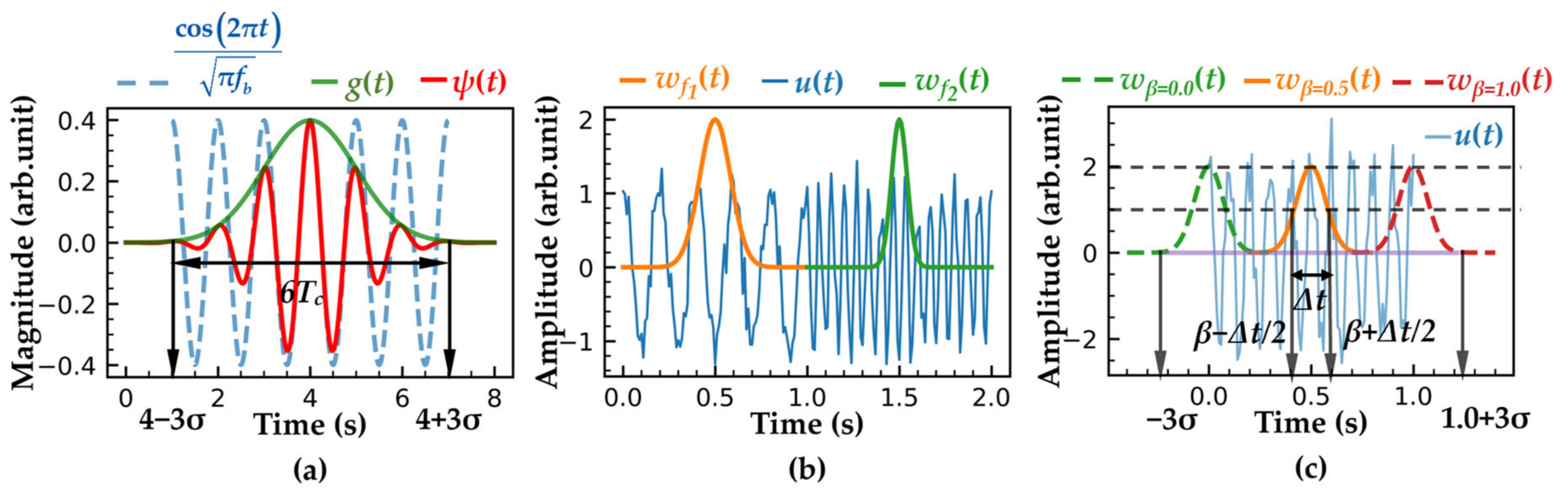
2.1. The Essence of CMOR Wavelet Transform

Wavelet function CMOR f_b − f_c is generally expressed as follows [23]:

$$\psi \left(t\right)=\frac{1}{\sqrt{\pi f_b}}{e}^{-\frac{t^2}{f_b}}{e}^{j2\pi f_{c}t}=g\left(t\right)\left[\cos \left(2\pi f_{c}t\right)+j\sin \left(2\pi f_{c}t\right)\right]$$

(4)

It can be found from Equation (4) that the real part of CMOR f_b − f_c is the product of the Gaussian function $g\left(t\right)$ and the cosine function, which has a center frequency f_c. As shown in Figure 1a, the support region of ψ(t) is defined by the “3σ” limits of Gaussian Distribution X~N (μ, σ²) [25]. The “3σ” limits mean that the area under the distribution curve between t = μ − 3σ and t = μ + 3σ is 0.9973 [26,27]. According to Equation (4), one can note the σ² and μ of Gaussian Distribution are f_b/2 and 0, respectively. Thus, the support region of ψ(t) is $\left(-3\sqrt{f_b/2},3\sqrt{f_b/2}\right)$. The real part of CMOR2-1 is shown in Figure 1a. Obviously, the cosine function (blue dotted line) is enveloped by the Gaussian function (green line) to form the real part of CMPR2-1 (red line) and there are 6T_c in the support region.

The CWT of u(t) is generally expressed as [28]:

$$CWT\left(\alpha ,\beta \right)=〈\frac{1}{\sqrt{\alpha }}\psi \left(\frac{t-\beta }{\alpha }\right),u(t)〉=〈{\psi }_{\alpha ,\beta }\left(t\right),u\left(t\right)〉$$

(5)

where α and β represent the dimensionless scale factor and the time translation factor, respectively. Plugging Equation (4) into Equation (5), the CMOR wavelet transform of u(t) is:

$$CMOR\left(\alpha ,\beta \right)=〈e^{j2\pi \left(\frac{f_c}{\alpha }\right)\left(t-\beta \right)},f\left(t\right)〉=F\left(\frac{f_c}{\alpha }\right)$$

(6)

where $f(t)=\frac{1}{\sqrt{\alpha \pi f_b}}{e}^{-\frac{{\left(t-\beta \right)}^2}{f_b{\alpha }^2}}u\left(t\right)=w\left(t\right)u\left(t\right)$. It can be found from Equation (6) that the essence for the CMOR wavelet transform of the signal u(t) is the FT of f(t). Moreover, f(t) is derived from the multiplication of u(t) and the window function w(t). Let the target frequency f_k = f_c/α, then the w(t) can be expressed as:

$$w\left(t\right)=\sqrt{\frac{f_k}{\pi f_c{f}_b}}{e}^{-\frac{f_k{}^2}{f_c{}^2{f}_b}{\left(t-\beta \right)}^2}$$

(7)

Obviously, w(t) is a Gaussian function and is dependent on the target frequency f_k. In Figure 1b, we illustrated how the window function w(t) with different support regions is applied to a signal. For the signal with lower frequency, the window function having a large support region (orange line) is applied. Otherwise, the window function having a small support region (green line) is applied to the signal with higher frequency.

By analogy with Equation (3), the CMOR wavelet transform of x(n) can be expressed as:

$$WT\left(\mathrm{s},\tau \right)={\displaystyle \sum _{n=0}^{N-1}\frac{1}{\sqrt{s\pi f_b}}{e}^{-\frac{{\left(n-\tau \right)}^2}{s^2{f}_b}}x\left(n\right)e^{-j2\pi \frac{f_c}{s}(n-\tau )}}$$

(8)

where s and τ represent the scale factor in Hz and the time translation factor, respectively. It can be found from Equations (3) and (8) that f_c/s = k/N = f_k/f_s, namely s = f_c f_s/f_k. Therefore, the relationship between s and α is s = αf_s.

2.2. Time-Frequency Resolution and Edge Effect

A previous study has shown that the time-frequency resolution of the CMOR wavelet transform depends on the full width at half maximum (FWHM) of the window function w(t) [28]. Based on the FWHM, the time resolution Δt is shown in Figure 1c. According to Equation (7), the following equation can be derived:

$$\frac{w\left(\beta \right)}{w\left(\beta +\frac{\mathrm{\Delta }t}{2}\right)}=\frac{1}{e^{-\frac{{\left(\mathrm{\Delta }t{f}_k\right)}^2}{4f_c^2{f}_b}}}=2$$

(9)

Therefore, the Δt is derived as:

$$\mathrm{\Delta }t=\frac{2\sqrt{\ln 2}{f}_c\sqrt{f_b}}{f_k}$$

(10)

The FT of the wavelet function ψ_{α, β}(t) is derived as follows:

$$\mathrm{\Psi }\left(f\right)=〈e^{j2\pi f\left(t-\beta \right)},{\psi }_{\alpha ,\beta }\left(t\right)〉=〈e^{j2\pi \left(f-f_k\right)\left(t-\beta \right)},w\left(t\right)〉=\sqrt{\frac{f_c}{f_k}}{e}^{-\frac{{\left(\pi f_c\right)}^2{f}_b}{f_k^2}{\left(f-f_k\right)}^2}$$

(11)

Obviously, Ψ(f) is a Gaussian function. The frequency resolution Δf is the FWHM of Ψ(f). According to Equation (11), the Δf is:

$$\mathrm{\Delta }f=\frac{2\sqrt{\ln 2}{f}_k}{\pi f_c\sqrt{f_b}}$$

(12)

According to Equations (10)–(12), we can find that $\mathrm{\Delta }t\mathrm{\Delta }f=\frac{4\ln 2}{\pi }>\frac{1}{4\pi }$, which satisfies the limit of the Heisenberg uncertainty principle.

As can be seen from Figure 1c, the window function w(t) can be completely multiplied by the signal u(t) when β is located in the middle instant of u(t) (the orange line). However, it only partially multiplied when β is located in the instant of signal appearance (t = 0.0 s, namely the green line) or disappearance (t = 1.0 s, namely the red line). That is the reason inducing the edge effect of CMOR wavelet transform. From Figure 1c, the total time of edge effect is δt = 6σ. Therefore, according to Equation (7), δt can be expressed as:

$$\delta t=\frac{3\sqrt{2}{f}_c\sqrt{f_b}}{f_k}$$

(13)

It can be found from Equations (10) and (13) that the total time of edge effect is obviously proportional to the time resolution.

2.3. CMOR Wavelet Parameters of Target Frequency

Assuming that the duration of one discrete signal is T₀ and the frequency nearest to the target frequency f_k is f_n, then the difference between f_k and f_n is $\delta f=\left|f_k-f_n\right|$, and the frequency resolution should satisfy the condition: ∆f < δf. According to Equation (12), the wavelet parameters f_b and f_c that satisfy this condition are:

$$f_c\sqrt{f_b}\ge \frac{2\sqrt{\ln 2}{f}_k}{\pi \delta f^{\prime }}>\frac{2\sqrt{\ln 2}{f}_k}{\pi \delta f}$$

(14)

where δf′ is a constant and 0 < δf′ < δf. As for the edge effect, available studies have shown that the limit of δt is δt ≤ 0.2T₀ [20,23]. According to Equation (13), the f_b and f_c that satisfy the limit of δt are:

$$f_c\sqrt{f_b}\le \frac{T_0{f}_k}{15\sqrt{2}}$$

(15)

Therefore, the optimal f_b and f_c for the target frequency f_k need to satisfy both Equations (14) and (15). Moreover, T₀ needs to meet the following condition:

$$\frac{30\sqrt{2\ln 2}}{\pi \delta f^{\prime }}\le T_0$$

(16)

When T₀ cannot satisfy Equation (16), the signal duration should be extended by padding with an equal number of zeros before the signal occurs and after its disappearance [29].

From Equations (10), (12), (13), we can find that as the value of $f_c\sqrt{f_b}$ increases, Δt and δt synchronously increase, while Δf reversely decreases. The optimal f_b and f_c for the target frequency need to meet the requirements of Δf, and the δt should be as small as possible. According to Equations (14) and (15), we therefore let $f_c\sqrt{f_b}=\frac{2\sqrt{\ln 2}{f}_k}{\pi \delta f^{\prime }}$. Theoretically, the f_b and f_c that meet this equation can not only satisfy the requirement of frequency resolution but also satisfy the limit of edge effect.

3. Simulation Results and Discussions

In this study, the CMOR wavelet transform is performed using Python’s module “PyWavelets” [30] and with the optimal f_b and f_c:

$$f_b=\frac{\sqrt{2\ln 2}{f}_k}{\pi \delta f^{\prime }},f_c=\sqrt{2f_b}$$

(17)

Equation (17) is derived from the separation of $f_c\sqrt{f_b}=\frac{2\sqrt{\ln 2}{f}_k}{\pi \delta f^{\prime }}$. With the definite f_b and f_c, we further perform the QTF analysis of water molecule vibration by CMOR wavelet transform based on the atomic trajectories from our first-principles molecular dynamics (FPMD) simulation. Under the framework of density functional theory, the FPMD simulation was performed with the quickstep module of CP2K code [31,32] with microcanonical ensemble. The triple-zeta valence Gaussian basis sets with two sets of polarization functions optimized for Goedecker–Teter–Hutter pseudopotentials [33] and the local density approximation exchange–correlation functional were used for H and O elements in H₂O molecule, with the cutoff energy of 280 Ry for the plane waves expansions. Under the periodic boundary conditions, a water molecule was placed in the center of a vacuum cube box, and the edge of the box was set to 15Å. The FPMD timestep is 0.1 fs. The total time of the FPMD simulation is 0.29 ns, which corresponds to 2.9 million MD steps. Here, the atomic trajectories of 1 million MD steps of H₂O molecule were used to perform the QTF analysis. Furthermore, details of the FPMD can be referred to in our previous study [34].

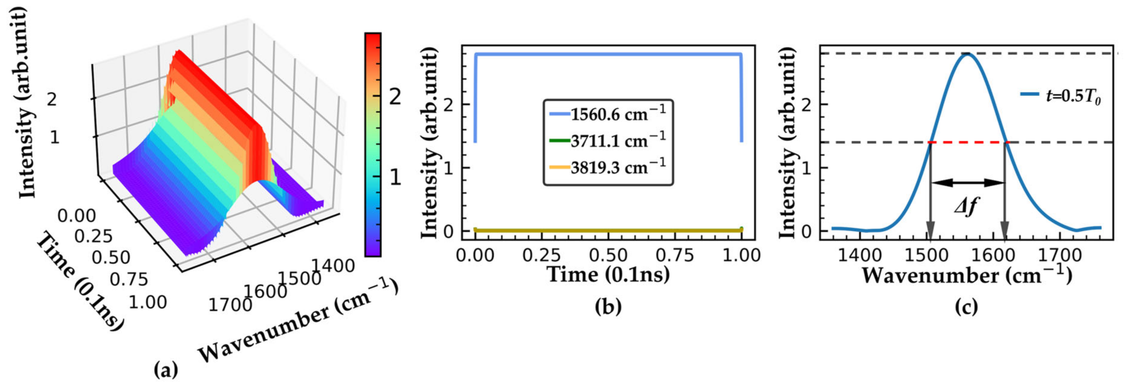
3.1. CMOR Wavelet Parameters for Water Molecule Vibration

In our previous study, the FT of the atomic trajectories indicated that the water molecule vibration includes three frequencies, namely, O-H bending vibration (1560.6 cm⁻¹), O-H symmetric stretching vibration (3711.1 cm⁻¹), and O-H asymmetric stretching vibration (3819.3 cm⁻¹) [34]. To select the appropriate f_b and f_c, the three vibrational frequencies of the water molecule here are represented as cosine signals, which are u₁(t) = cos(2π1560.6v_ct), u₂(t) = cos(2π3711.1v_ct), and u₃(t) = cos(2π3819.3v_ct) in order. The v_c represents the speed of light in cm/s. The signal duration is T₀ = 10⁻¹⁰ s and the sampling frequency f_s = 5 × 10¹⁴ Hz.

For O-H bending vibration, it is clear that f_k = 1560.6 cm⁻¹, f_n = 3711.1 cm⁻¹, and δf = 2150.5 cm⁻¹. Let δf′ = 100.0 cm⁻¹; then, we can get 3.75 × 10⁻¹² s < 10⁻¹⁰ s by plugging δf′ and T₀ into Equation (16). This indicates that it is unnecessary to extend the signal duration. By plugging the values of f_k and δf′ into Equation (17), we can get f_b = 6.0 and f_c = 3.0. Consequently, the CMOR wavelet transform of O-H bending vibration is shown in Figure 2.

It can be seen from Figure 2a that the target frequency f_k always has the maximum intensity over the signal duration T₀. From Figure 2b, the intensity of 3711.1 cm⁻¹ and 3819.3 cm⁻¹ are both close to zero. The edge effect of 1560.6 cm⁻¹ is almost negligible. From Figure 2c, we can find that Δf < δf. These results indicate that f_b = 6.0 and f_c = 3.0 given by Equation (17) are the optimal wavelet parameters for the target frequency f_k. Similarly, the optimal CMOR wavelet parameters for the symmetric and asymmetric stretching vibration of O-H were also derived from Equation (17) and listed in

Table 1. Optimal wavelet parameters for water molecule vibration.

Wavenumber (cm −1)	δf (cm −1)	δf′ (cm −1)	fb	fc	Δf (cm −1)	δt (10 −10 s)
1560.6	2150.5	100.0	6.0	3.0	113	0.00667
3711.1	108.2	70.0	20.0	6.0	74	0.01024
3819.3	108.2	60.0	24.0	7.0	59	0.01271

. As shown in Table 1, the CMOR wavelet parameters of f_b = 20.0 and f_c = 6.0 for symmetric stretching vibration are obtained when the artificial δf′ = 70.0 cm⁻¹ is set. Obviously, we can find that Δf = 74 cm⁻¹ and δt = 1.024 × 10⁻¹² s are smaller than δf = 108.2cm⁻¹ and 0.2T₀, respectively. Similar results can be obtained from the CMOR parameters f_b = 24 and f_c = 7.0 of asymmetric stretching vibration. These results show that the CMOR wavelet parameters of symmetric and asymmetric stretching vibration not only satisfy the requirement of frequency resolution but also satisfy the limit of edge effect.

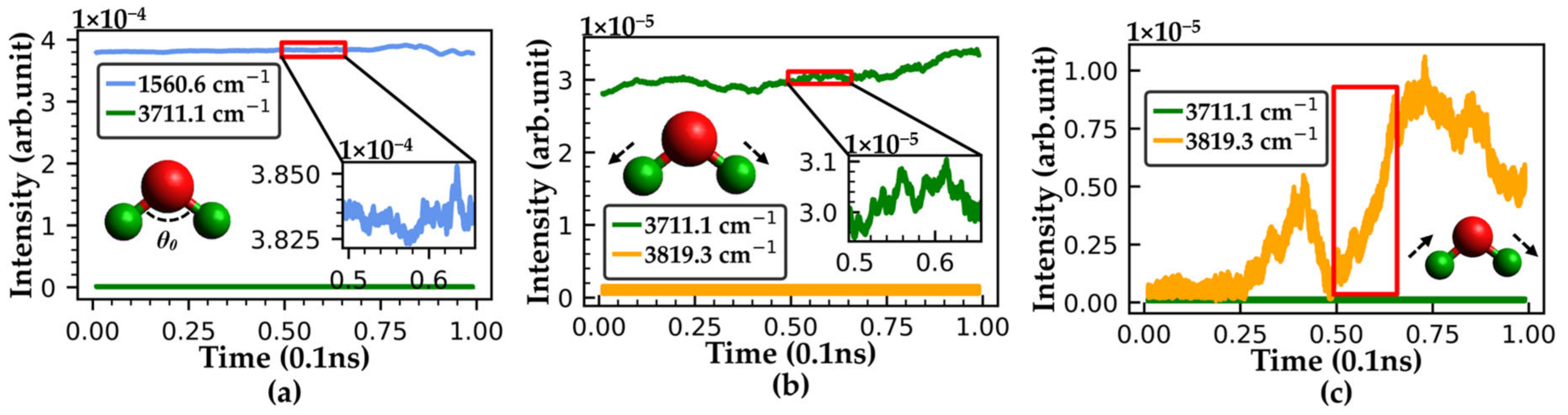
3.2. Quantitative Time-Frequency Analysis of Water Molecule

Based on the derived optimal wavelet parameters, the QTF analysis of the water molecule vibration is performed with CMOR wavelet transform in this part, and the results are shown in Figure 3. The frequency of each target vibration mode is assigned as f_k. Moreover, the intensity of f_k over time is given by the CMOR wavelet transform of H-atom trajectories. One cosine signal is constructed to represent the vibration mode with a frequency nearest to f_k. The frequency of this cosine signal is f_n.

Obviously, it can be found from Figure 3 that in the initial stage of the FPMD simulation (t < 0.2T₀), the water molecule vibrations are mainly dominated by the O-H bending, which is accompanied by a slight symmetric stretching vibration. However, the intensity of the O-H asymmetric stretching vibration significantly increases when t > 0.5T₀, as shown in Figure 3c. It indicates that there is an uphill energy relaxation in the water molecule vibration; namely, the lower frequency vibration mode can excite the higher one. Experimentally, 2D-IR and pump-probe measurements reveal that strong couplings of water molecular vibration allow bend excitation to drive stretching motions (up-pumping) and downhill energy relaxation pathway that form the bend to low-frequency modes [35,36]. Therefore, our result agrees well with the experimental result, which in turn further confirms the feasibility and reliability of our selection method for the optimal CMOR wavelet parameters.

4. Conclusions

In this paper, we have clearly demonstrated that the essence of the CMOR wavelet transform is the windowed Fourier transform. The shape of the window function is highly related to the target frequency. We propose a feasible and reliable method for the selection of the optimal wavelet parameters of f_b and f_c. Taking the vibrational modes of the water molecule as an example, the CMOR wavelet parameters obtained by our method can not only meet the requirement of frequency resolution but also meet the limit of edge effect. Further QTF analysis indicates that there is an uphill energy relaxation in the vibration of the water molecule, which is consistent with the experiment. The method proposed in this paper will make the application of CMOR wavelet transform more convenient.

References

1. Varanis, M.; Silva, A.L.; Balthazar, J.M.; Pederiva, R. A tutorial review on time-frequency analysis of non-stationary vibration signals with nonlinear dynamics applications. Braz. J. Phys. 2021, 51, 859–877. [Google Scholar] [CrossRef]
2. Li, H.; Lv, H.; Gu, J.; Xiong, J.; Han, Q.; Liu, J.; Qin, Z. Nonlinear vibration characteristics of fibre reinforced composite cylindrical shells in thermal environment. Mech. Syst. Signal Process. 2021, 156, 107665. [Google Scholar] [CrossRef]
3. Gao, J.; Song, Q.; Liu, Z. Chatter detection and stability region acquisition in thin-walled workpiece milling based on CMWT. Int. J. Adv. Manuf. Technol. 2018, 98, 699–713. [Google Scholar] [CrossRef]
4. Wei, D.; Hu, M. Theory and applications of short-time linear canonical transform. Digit. Signal Process. 2021, 118, 103239. [Google Scholar] [CrossRef]
5. Feng, Z.; Liang, M.; Chu, F. Recent advances in time–frequency analysis methods for Machinery Fault Diagnosis: A review with application examples. Mech. Syst. Signal Process. 2013, 38, 165–205. [Google Scholar] [CrossRef]
6. Cohen, L. Time-frequency distributions-A Review. Proc. IEEE 1989, 77, 941–981. [Google Scholar] [CrossRef] [Green Version]
7. Rioul, O.; Flandrin, P. Time-scale energy distributions: A general class extending wavelet transforms. IEEE Trans. Signal Process. 1992, 40, 1746–1757. [Google Scholar] [CrossRef]
8. Baraniuk, R.G.; Jones, D.L. A signal-dependent time-frequency representation: Optimal Kernel Design. IEEE Trans. Signal Process. 1993, 41, 1589–1602. [Google Scholar] [CrossRef]
9. Rodríguez Fonollosa, J.; Nikias, C.L. Analysis of finite-energy signals higher-order moments- and spectra-based time-frequency distributions. Signal Process. 1994, 36, 315–328. [Google Scholar] [CrossRef]
10. Stankovic, L.J. L-class of time-frequency distributions. IEEE Signal Process. Lett. 1996, 3, 22–25. [Google Scholar] [CrossRef]
11. Stankovic, L.J. S-class of time–frequency distributions. IEEE Proc. Vis. Image Signal Process. 1997, 144, 57. [Google Scholar] [CrossRef]
12. Huang, N.E.; Wu, Z. A review on Hilbert-Huang Transform: Method and its Applications to Geophysical Studies. Rev. Geophys. 2008, 46, 2. [Google Scholar] [CrossRef] [Green Version]
13. Ramasesha, K.; De Marco, L.; Mandal, A.; Tokmakoff, A. Water vibrations have strongly mixed intra- and intermolecular character. Nat. Chem. 2013, 5, 935–940. [Google Scholar] [CrossRef] [PubMed]
14. De Marco, L.; Fournier, J.A.; Thämer, M.; Carpenter, W.; Tokmakoff, A. Anharmonic exciton dynamics and energy dissipation in liquid water from two-dimensional infrared spectroscopy. J. Chem. Phys. 2016, 145, 094501. [Google Scholar] [CrossRef] [PubMed]
15. Matt, S.M.; Ben-Amotz, D. Influence of intermolecular coupling on the vibrational spectrum of water. J. Phys. Chem. B 2018, 122, 5375–5380. [Google Scholar] [CrossRef] [PubMed]
16. Rhif, M.; Ben Abbes, A.; Farah, I.; Martínez, B.; Sang, Y. Wavelet transform application for/in Non-Stationary Time-Series Analysis: A Review. Appl. Sci. 2019, 9, 1345. [Google Scholar] [CrossRef] [Green Version]
17. Cohen, M.X. A better way to define and describe Morlet wavelets for time-frequency analysis. NeuroImage 2019, 199, 81–86. [Google Scholar] [CrossRef]
18. Dinç, E.; Baleanu, D. A review on the wavelet transform applications in analytical chemistry. Math. Methods Eng. 2007, 265–284. [Google Scholar]
19. Yan, B.F.; Miyamoto, A.; Brühwiler, E. Wavelet transform-based modal parameter identification considering uncertainty. J. Sound Vib. 2006, 291, 285–301. [Google Scholar] [CrossRef]
20. Gaviria, C.A.; Montejo, L.A. Optimal wavelet parameters for system identification of civil engineering structures. Earthq. Spectra 2018, 34, 197–216. [Google Scholar] [CrossRef]
21. Deák, D.K.; Kocsis, K.I. Complex morlet wavelet design with global parameter optimization for diagnosis of industrial manufacturing faults of tapered roller bearing in noisycondition. Diagnostyka 2019, 20, 77–86. [Google Scholar] [CrossRef]
22. Li, W.; Huang, Q.-A.; Yang, C.; Chen, J.; Tang, Z.; Zhang, F.; Li, A.; Zhang, L.; Zhang, J. A fast measurement of Warburg-like impedance spectra with Morlet wavelet transform for electrochemical energy devices. Electrochim. Acta 2019, 322, 134760. [Google Scholar] [CrossRef]
23. Năstac, S.; Debeleac, C.; Simionescu, C. Dynamic diagnosis of elastic coupling transmissions of technological equipments based on joint time-frequency evaluations. Appl. Mech. Mater. 2014, 657, 465–469. [Google Scholar] [CrossRef]
24. Blair, G.M. A review of the discrete Fourier transform. part 1: Manipulating the powers of two. Electron. Commun. Eng. J. 1995, 7, 169–177. [Google Scholar] [CrossRef]
25. DasGupta, A.; Casella, G.; Fienberg, S.; Olkin, I. Normal Distribution. In Fundamentals of Probability a First Course; Springer: New York, NY, USA, 2010; pp. 195–212. [Google Scholar]
26. Goh, T.N. Some common measurement limits used in quality control. Int. J. Qual. Reliab. Manag. 1986, 3, 21–30. [Google Scholar] [CrossRef]
27. Rosaiah, K.; Rao, B.S.; Reddy, J.P.; Chinnamamba, C. Variable control charts for Gumbel Distribution based on percentiles. J. Comput. Math. Sci. 2018, 9, 1890–1897. [Google Scholar] [CrossRef]
28. Brian, R.; Jiajun, H. Jean Morlet and the continuous wavelet transform. CREWES Res. Rep. 2016, 28, 115. Available online: https://www.crewes.org/Documents/ResearchReports/2016/CRR201668.pdf (accessed on 16 October 2022).
29. Pal, M.P.; Panigrahi, P.K. A multi scale time–frequency analysis on electroencephalogram signals. Phys. A Stat. Mech. Its Appl. 2022, 586, 126516. [Google Scholar] [CrossRef]
30. Lee, G.; Gommers, R.; Waselewski, F.; Wohlfahrt, K.; O’Leary, A. PyWavelets: A python package for Wavelet Analysis. J. Open Source Softw. 2019, 4, 1237. [Google Scholar] [CrossRef]
31. Hutter, J.; Iannuzzi, M.; Schiffmann, F.; Vondele, J.V. Cp2k: Atomistic simulations of condensed matter systems. Wiley Interdiscip. Rev. Comput. Mol. Sci. 2014, 4, 15–25. [Google Scholar] [CrossRef] [Green Version]
32. Vondele, J.V.; Krack, M.; Mohamed, F.; Parrinello, M.; Chassaing, T.; Hutter, J. Quickstep: Fast and accurate density functional calculations using a mixed Gaussian and plane waves approach. Comput. Phys. Commun. 2005, 167, 103–128. [Google Scholar] [CrossRef] [Green Version]
33. Goedecker, S.; Teter, M.; Hutter, J. Separable dual-space gaussian pseudopotentials. Phys. Rev. B 1996, 54, 1703–1710. [Google Scholar] [CrossRef] [PubMed] [Green Version]
34. Wang, S. Efficiently calculating anharmonic frequencies of molecular vibration by molecular dynamics trajectory analysis. ACS Omega 2019, 4, 9271–9283. [Google Scholar] [CrossRef] [PubMed] [Green Version]
35. Carpenter, W.B.; Fournier, J.A.; Biswas, R.; Voth, G.A.; Tokmakoff, A. Delocalization and stretch-bend mixing of the Hoh Bend in Liquid Water. J. Chem. Phys. 2017, 147, 84503. [Google Scholar] [CrossRef]
36. Yu, C.-C.; Chiang, K.-Y.; Okuno, M.; Seki, T.; Ohto, T.; Yu, X.; Korepanov, V.; Hamaguchi, H.-O.; Bonn, M.; Hunger, J.; et al. Vibrational couplings and energy transfer pathways of water’s bending mode. Nat. Commun. 2020, 11, 5977. [Google Scholar] [CrossRef]
Figure 1. The essence of CMOR wavelet transform. (a) The real part of CMOR2-1, (b) The window functions corresponding to different target frequencies (f1, f2) in u(t), (c) Time resolution and edge effect of CMOR wavelet.
Applsci 13 02734 g001
Figure 2. The CMOR wavelet transform of cosine signal (O-H bending vibration): (a) The 3D time-frequency analysis, (b) The intensity variation over time for fk, (c) Intensity of various frequencies at 0.5T0f = 113 cm−1).
Applsci 13 02734 g002
Figure 3. QTF analysis of the water molecule vibration: (a) O-H bending vibration (fk = 1560.6 cm−1, fn = 3711.1 cm−1), (b) O-H symmetric stretching vibration (fk = 3711.1 cm−1, fn = 3819.3 cm−1), (c) O-H asymmetric stretching vibration (fk = 3819.3 cm−1, fn = 3711.1 cm−1).
Applsci 13 02734 g003