Article

Trajectory Tracking of Autonomous Vehicle Using Clothoid Curve

1
Department of Vehicle Engineering, Army Military Transportation University, No. 1 Chenglin Street, Tianjin 300161, China
2
Institute of Military Transportation, Army Military Transportation University, Tianjin 300161, China
*
Authors to whom correspondence should be addressed.
Appl. Sci. 2023, 13(4), 2733; https://doi.org/10.3390/app13042733
Submission received: 13 January 2023 / Revised: 14 February 2023 / Accepted: 17 February 2023 / Published: 20 February 2023

Abstract

:
This paper proposes a clothoid-curve-based trajectory tracking control method for autonomous vehicles to solve the problem of tracking errors caused by the discontinuous curvature of the control curve calculated by the pure pursuit tracking algorithm. Firstly, based on the Ackerman steering model, the motion model is constructed for vehicle trajectory tracking, Then, the position of the vehicle after the communication delay of the control system is predicted as the starting point of the clothoid control curve, and the optimization interval of the curve end point is determined. The clothoid control curves are calculated, and their parameters are verified by the vehicle motion and safety constraints, so as to obtain the optimal clothoid control curve satisfying the constraints. Finally, considering the servo system response delay time of the steering system, the steering angle target control value is obtained by previewing the curvature of the clothoid control curve. The field experiment is conducted on the test road, which consists of straight, right-angle turns and lane-change elements under three sets of speed limitations, and the test results show that the proposed clothoid-curve-based trajectory tracking control method greatly improved the tracking accuracy compared with the pure pursuit method; in particular, the yaw deviation is improved by more than 50%.

1. Introduction

Accurate and smooth motion control is a key technology to ensure the safety and comfort of autonomous vehicles. Vehicle motion control can be further divided into longitudinal speed control and lateral trajectory tracking. Trajectory tracking of autonomous driving has been widely studied in industry and academia alike [1,2,3,4]. This problem can be summarized into two major research contents: the control model and the control method. Control models mainly include geometric models, kinematic models, dynamic models, etc. Control methods include geometric methods, feedforward and feedback control methods [5], Lyapunov direct methods [6], robust control methods [7], intelligent control methods [8], etc. Thanks to properties such as low model complexity, few parameters, and low computation consumption, the geometric model and the control method have been widely used. The pure pursuit tracking method is the most popular geometric control method that has been studied and applied the most in recent years [9,10,11]. However, its planned control curve is an arc segment and does not consider the constraint of the actual vehicle control on the continuity of the path curvature. In addition, the algorithm uses a certain preview distance selection strategy that has poor adaptability to paths with different curvatures.
This paper introduces a method that constructs a vehicle motion model with a continuous curvature path and provides a new control law that uses a G2 continuous clothoid curve to improve the tracking accuracy and ride comfort experience for the trajectory tracking task of an autonomous vehicle. The overall flow of the algorithm is shown in Figure 1. First, the vehicle state is predicted by the communication delay of the control system, and then the starting and ending points of the clothoid curve are determined according to the vehicle state and the parameters of the reference path. The clothoid curve is calculated using the method given in Reference [12]. This method is reliable and quick and can reach the microsecond level. The parameters of the clothoid curves are checked for feasibility constraints, and the optimal control curve is obtained. Then, the response hysteresis of the steering system that is controlled through the CAN bus is taken into consideration; finally, the preview control method based on the clothoid curve is proposed. The correctness of the approach proposed in this paper can be checked by simulation and experiment. The simulation verification can adopt the concept of model-based testing [13,14]. In this paper, we directly use field experiments to check the correctness of the approach. The field experiment consists of comparative tests in various curved-road environments in a park. The experimental results show that the trajectory tracking control method based on the clothoid curve proposed in this paper greatly improved the tracking accuracy at different speeds compared with the pure pursuit method.
The rest of this paper is organized as follows. In Section 2, the related literature on the geometric vehicle model, control curve, and control system delay are discussed. Section 3 details the steps taken to calculate the steering wheel angle based on the clothoid control curve. Section 4 details the experiments conducted on an actual vehicle and analyzes the accuracy and advantages of the method proposed in this paper. The last section concludes the work and discusses further research.

2. Related Work

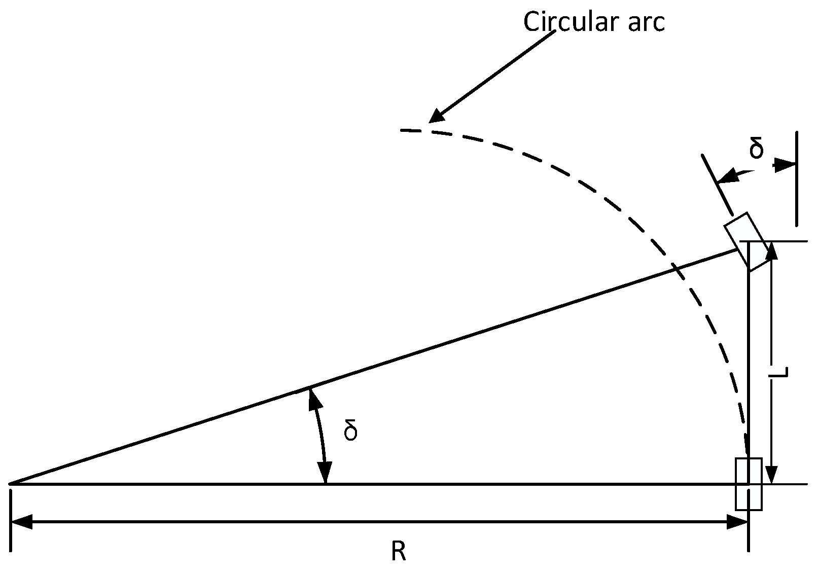
2.1. Geometric Vehicle Model

Usual vehicle model configurations consist of geometric, kinematic, and dynamic models. The geometric vehicle model is particularly important in order to relate the vehicle’s dimensions, the radius of the turn, and the radius of the curvature of the road undertaken by the vehicle during turning. It is developed based on Ackerman steering configurations, where the line perpendicular to each of the vehicle wheels should intersect at the center point of the vehicle cornering arc where the radius of turn is R (Figure 2). This model only considers the dimension and positions of the vehicle with no regard to its velocity, acceleration, and internal forces [2]. Therefore, compared with the kinematics and dynamics models, using this model for trajectory tracking control usually has the highest computational efficiency. However, large-tire lateral forces and lateral acceleration will be produced when the vehicle turns at high speed, which cannot be neglected; therefore, if geometric vehicle models are used for trajectory tracking control, vehicle speed must be limited when passing curves in order to ensure high trajectory tracking accuracy.

2.2. Control Curve

The reference path obtained from the path planning module is used as the target curve of the trajectory tracking module. The general approach of the geometric controller is to select a preview point on the reference path, plan a curve from the current vehicle position to the preview point, and calculate the target angle of the steering wheel according to the geometric model of the vehicle, so as to realize the lateral control of the vehicle in the path tracking process. Pure pursuit as the most popular geometric trajectory tracking method uses an arc to connect the current position of the vehicle and the preview point on the reference path as the control curve, ignoring the constraint of the vehicle’s path on the curvature continuity, which will lead to tracking deviation in theory. Wit et al. proposed a trajectory tracking method based on the spiral theory, which considered both the position and direction of the vehicle at the target point [15], but this method is not widely used due to its complexity. Amidi et al. proposed using a quintic polynomial to draw the planned control curve, taking into account the position, direction, and curvature constraints of the starting and ending points [16]. This method does not guarantee a feasible solution and has high computational complexity, so it is not widely used. Girb et al. [17] and Shan et al. [18] both mentioned to use a clothoid curve to fit the control curve between the current position of the vehicle and the preview point. The most important feature of a clothoid curve is that its parameter function satisfies the continuity on the second derivative; that is, the curvature change in the curve is continuous. In fact, the curvature of the clothoid curve is proportional to the arc length of the curve, making it highly popular in highway or railway design to ease the curvature change between straight and circular routes. The general form of the clothoid curve parameter equation can be described as [18].
{ x ( s ) = x 0 + [ 0 s cos ( 1 2 κ τ 2 + κ τ + θ 0 ) d τ ] y ( s ) = y 0 + [ 0 s sin ( 1 2 κ τ 2 + κ τ + θ 0 ) d τ ] ,
where s represents the arc length of the curve, x 0 and y 0 represent the starting point coordinates of the curve, θ 0 represents the deflection angle of the starting point of the curve, κ represents the curvature at the starting point of the curve, and κ represents the curvature change rate of the curve.
Compared with other curve fitting methods, using a clothoid curve to plan the vehicle control path has the advantages as follows.
  • When the driver controls the steering wheel, in order to ensure lateral stability, the steering wheel is generally controlled at a constant speed, which means the angular speed of the steering wheel is constant. When the speed and front wheel angle change are very small in a tiny period of time and can be ignored, the change rate of the path curvature is constant, which is consistent with the characteristics of the clothoid curve. Therefore, the planned control path constructed by the clothoid curve can ensure that the vehicle control process is stable and the jitter is tiny.
  • The clothoid curve satisfies the G2 continuity conditions. Compared with the arc curve constructed by the pure pursuit tracking algorithm, the curvature of the starting point of the curve is consistent with the initial turning curvature of the vehicle, which can reduce tracking deviation at the beginning period of the path.
  • Compared with the polynomial curve, because its curvature changes linearly and continuously, it is easier to control and verify the curvature and curvature change rate of the planned control path and other constraints or limitations.

2.3. Control System Delay and Hysteresis

The steering control command generated by the control module needs to go through multiple nodes, such as the processing of the interface driver and the CAN bus transmission, which will bring in the communication delay of the control command. It also takes a certain amount of time for the steering servo system to receive the steering control CAN command and drive the actuator to achieve the target angle. This response time is called the response hysteresis of the steering system. The communication delay of the control system and the response delay of the steering system result in a situation where the control command cannot be realized immediately. If proper compensation is not made, it would cause the system to become unstable or limit the speed of the autonomous vehicle [19]. Therefore, this paper proposes a vehicle future state prediction method to deal with the control system delay phenomenon, and proposes a preview control method based on the clothoid curve combined with the response hysteresis problem of the steering system.

3. Tracking Control Method Using Clothoid Curve

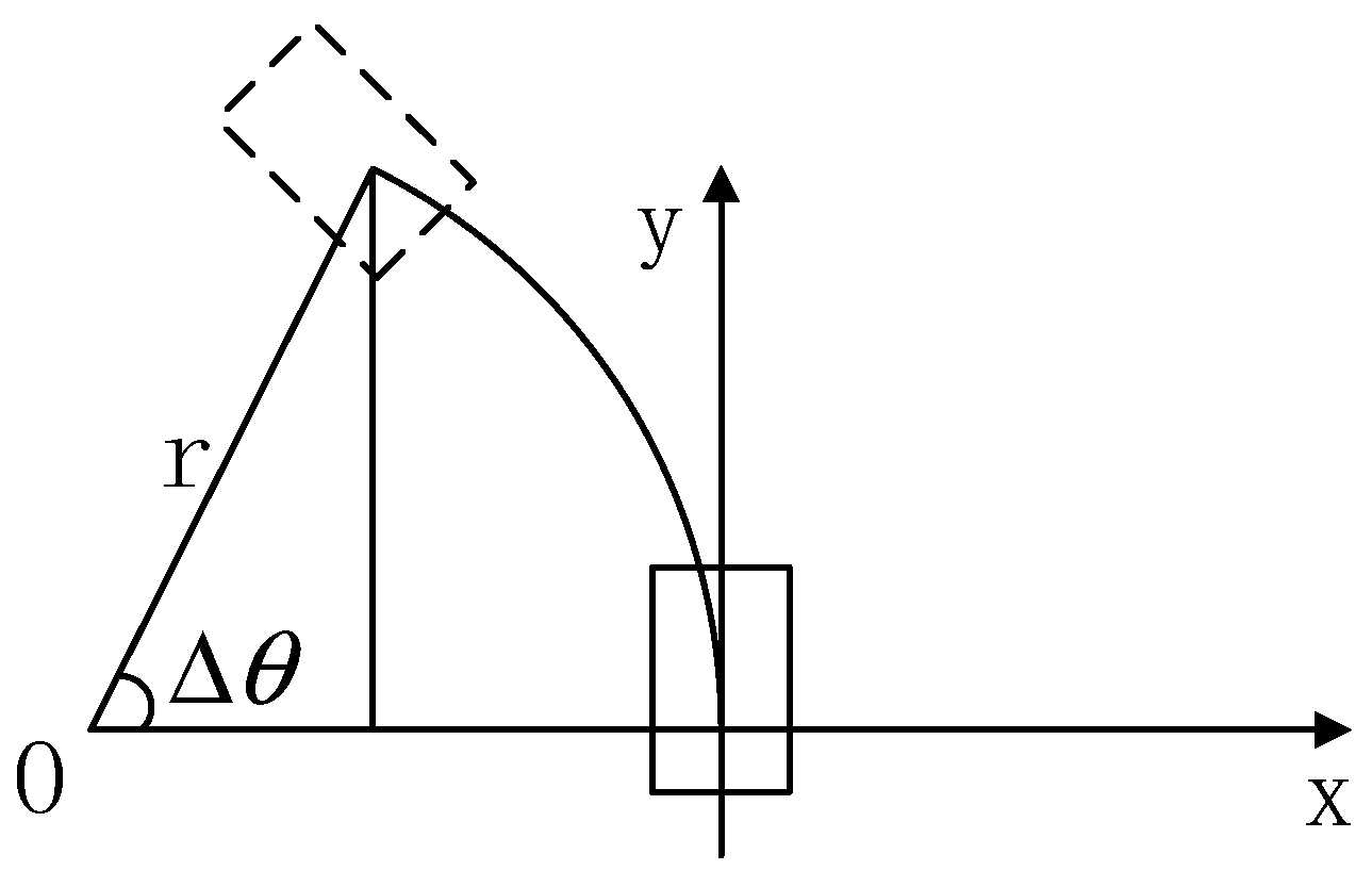
3.1. Kinematic Model of Vehicle Lateral Control

As shown in Figure 2, the relationship between the front wheel angle, wheelbase, and turning curvature of the vehicle can be obtained from the geometric relationship of the Ackerman steering vehicle, which can be described as
κ = tan ( δ ) L ,
where δ represents the front wheel angle, L represents the wheelbase, and κ represents the current turning curvature.
The change rate of curvature with time can be described as
d κ dt = d κ ds d s dt = κ v ,
where s represents the distance traveled in a tiny time period. Suppose that the vehicle travels at a constant speed v within this distance, and κ represents the change rate of curvature with arc length.
By substituting (3) with (2), we can obtain
d κ dt = d ( tan δ ) L * dt = κ v ,
Then we can obtain
κ = d ( δ ) / d t L v cos 2 ( δ ) ,
where d ( δ ) / d t represents the front wheel steering angular velocity. There is a linear proportional relationship between the angular velocity of the steering wheel and the front wheel, which can be described as
ω = k d ( δ ) / d t ,
where k represents the transmission ratio coefficient of the steering system, and ω represents the angular speed of the steering wheel. Therefore, the relationship between steering angular velocity of the steering wheel and the change rate of the vehicle motion curvature can be expressed as
κ = ω k L v cos 2 ( δ ) ,
As can be seen from Formula (7), since ω has an upper limit constraint by the steering system, it determines that the path curvature of the actual turning cannot change suddenly. Therefore, the curve used to control vehicle driving shall ensure its curvature continuity. Otherwise, tracking error would be inevitably produced between the actual vehicle motion and the reference path.

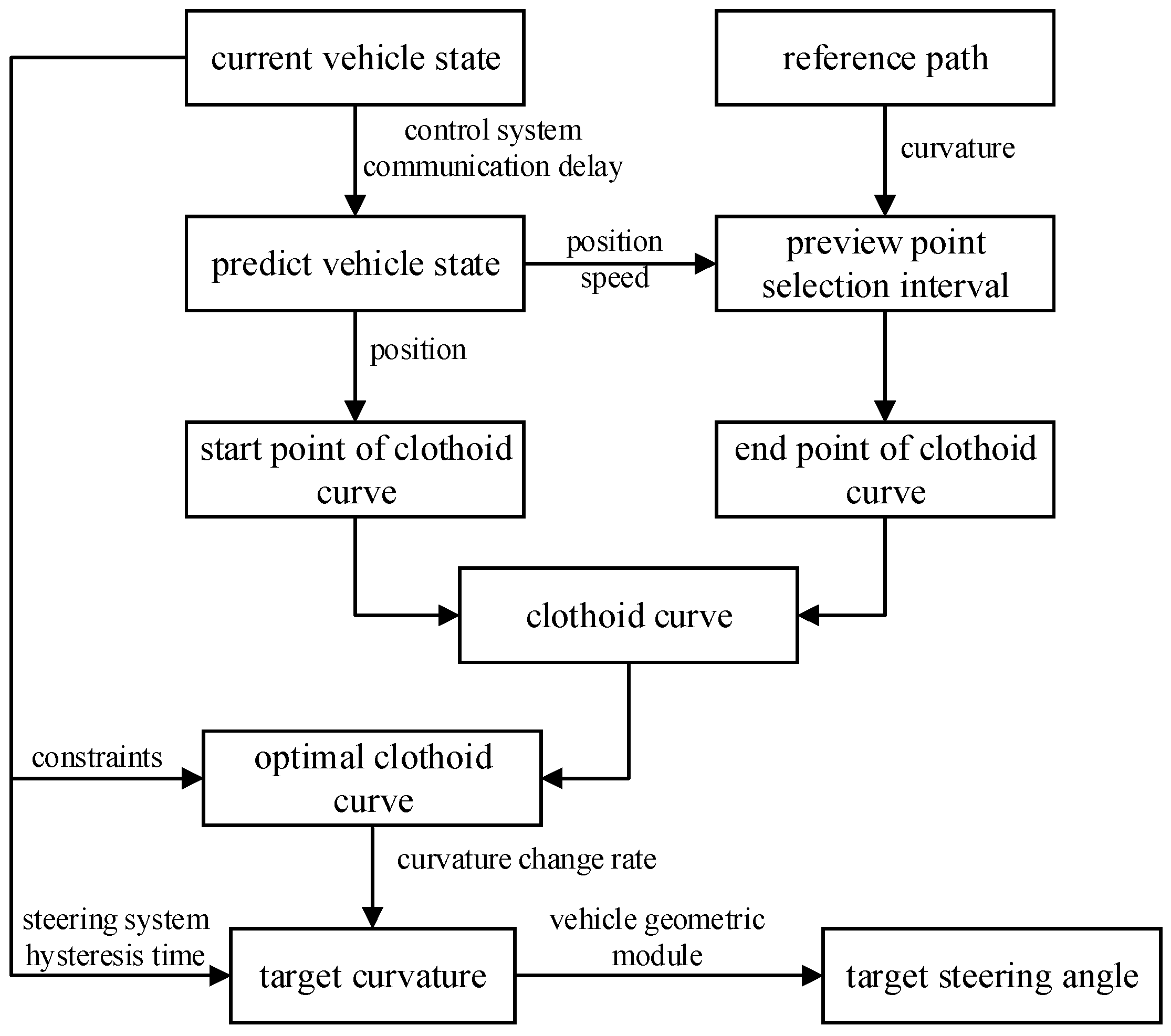
3.2. Algorithm Process

The overall process of the trajectory tracking control method based on the clothoid curve is shown in Algorithm 1. Firstly, the reference path is obtained from the path planning module. Then, it is checked whether the point number of the reference path is more than one. If not, the target steering angle calculated from the previous cycle is output; otherwise, the state of the vehicle after t1 is predicted according to the current state of the vehicle, where t1 is the communication delay time of the control system. The point closest to the predicted vehicle position on the reference path is found and set as the first point on the preview point selection interval; then, the last point of the preview point selection interval on the reference path is determined. The clothoid curve is calculated from the predicted vehicle position to the preview point, which is selected from the preview point selection interval. The clothoid curve obtained is composed of three curves. Since the distance traveled by the vehicle in the control cycle is covered by the first curve, only the parameters of the first S[0] curve need to be verified. If S[0] meets the vehicle motion and safety constraints, it would be used as the candidate curve; then, the process would jump to Step 6 to calculate the next clothoid curve. If the S[0] curve obtained does not satisfy the constraints, the validation of the existing candidate curve is checked. If it is valid, it is selected as the control curve; otherwise, the maximum curvature change rate under the limit is used as the change rate of the output curve, and its symbol should be consistent with S[0]. Taking the change rate of output curve curvature as a parameter, and taking the curvature of the corresponding position of the output curve after the preview t2 time of the current vehicle speed as the target curvature, the target angle of the front wheels of the vehicle is calculated and then converted to the steering wheel angle. Finally, the steering wheel control target angle is processed by the moving average filtering of the calculated steering wheel target angles from the processes above.
Algorithm 1: Trajectory tracking of autonomous vehicle using clothoid curve
Applsci 13 02733 i001

3.3. Vehicle State Prediction Based on Communication Delay

Due to the communication delay t1 of the control system, the control command sent at the current time cannot be responded to until t1. Therefore, the sent control command should also be calculated according to the state relationship between the vehicle and the reference path after t1, so it is necessary to predict the vehicle state after t1. Zakaria et al. proposed to move forward along the current longitudinal axis of the vehicle to predict the future state of the vehicle for tracking error calculation [20]. AbdElmoniem et al. proposed to predict the vehicle state in the following control cycles by using the vehicle’s current state vector [ X f , Y f , θ , V , δ ] , which are the vehicle’s current horizontal and coordinate position, heading angle, speed, and front wheel angle [21]. Xu et al. used the optimal control theory of the discrete time-delay system for reference, used the vehicle dynamics model to predict the state of vehicles in each cycle of the delay time in turn according to the control cycle, and also used the same front wheel angle in the prediction space of each control cycle, but the prediction accuracy of this method is affected by the accuracy of the vehicle dynamics model [19].
This paper needs to predict the state of the vehicle after the communication delay time t1 of the control system. The communication delay time t1 is about 0.1 s according to the test. During this time, the change in vehicle speed and front wheel angle are very small and can be ignored. Therefore, this paper uses the current state [ X , Y , θ , δ , v ] of the vehicle to predict the state of the vehicle after t1, which can ensure the calculation error in a small range.
Firstly, the position of the vehicle after t1 in the current vehicle frame is predicted, as shown in Figure 3. The state of the vehicle after t1 is calculated from the following geometric relationship:
{ s = v t 1 r = L / tan δ Δ θ = s / r Δ x = ( 1 cos ( Δ θ ) ) r Δ y = r sin Δ θ κ = κ v ,
Suppose that the vehicle keeps the current front wheel angle moving at a constant speed in time t1, where r is the current turning radius, L is the wheelbase, κ and κ v are the current turning curvature, v is the speed, and δ is the front wheel angle. At t1, s is the arc length, and the vehicle state can be expressed as [ Δ x , Δ y , Δ θ , κ ] , namely, the state of the vehicle in the current vehicle frame after time t1.
Since the frame of the reference path is the global coordinate system, the predicted vehicle state after time t1 in the current vehicle frame should also be converted to the global coordinate system.
{ x g = Δ x cos θ v Δ y sin θ v + x v y g = Δ x sin θ v + Δ y cos θ v + y v θ g = θ v + Δ θ κ g = κ v ,
where, [ x v , y v , θ v , κ v ] is the current state of the vehicle in the global coordinate system, and [ x g , y g , θ g , κ g ] is the predicted state of the vehicle in the global coordinate system in time t1.

3.4. Preview Point Selection

The state of the vehicle after the control system communication delay time t1 is obtained through prediction calculation, and the predicted vehicle position is taken as the starting point of the planned control path. The selection of the end point of the planned control path (also known as the preview point) will affect the deviation between the planned control path and the reference path (as shown in Figure 4). The closer the preview point is selected, the smaller the area enclosed by the planned control path and the reference path is, that is, the smaller the overall deviation of the trajectory tracking process. However, if the tracking control path is too short, the curvature and curvature change rate of the calculated clothoid curve might be too large, which will exceed the control range of the vehicle steering wheel angle and angular velocity, or cause the steering wheel angle to change dramatically, thus affecting the vehicle stability. Therefore, this paper proposes to design a preview point scanning interval. In this interval, the point that is closest to the predicted vehicle position and can satisfy the vehicle’s control non-integrity, safety, and stability constraints is found as the preview point to calculate the clothoid curve.
The point closest to the predicted vehicle position on the reference path is selected as the first point on the preview point interval. The last point on the preview point interval is calculated from the speed and the bending degree of the target curve. The specific de termination method is shown in Algorithm 2.
Algorithm 2: End point selection of preview point interval
Applsci 13 02733 i002
Set the initial value of the preview point selection interval length as s_init, then s_length is adjusted according to the vehicle speed and the curvature and length of the reference path. Next, set the point closest to the predicted vehicle position found on the reference curve as the start point, and search along the reference path to find the point whose distance to the start point is closest with s_length as the last point of the preview point selection interval.
After determining the preview point selection interval, calculate the clothoid curve from far to near points within the interval, and check whether the parameters of the curve obtained meet the constraints. The curve that can meet the constraints and its end point is closest to the predicted vehicle position is the optimal planned control path.

3.5. Constraints

The autonomous vehicle platform with Ackerman steering is used in the test of this paper. The motion constraints for the test platform include the maximum curvature and the maximum curvature change rate. In addition, the length of the planned control path designed by the clothoid curve should be long enough; otherwise, direction jitter will occur in the continuous control process.

3.5.1. Curvature Constraint

The maximum curvature constraint is discussed in two cases: stationary or low-speed state and normal running state. When the vehicle is stationary or moving at a very low speed, the maximum front wheel angle parameter is used to calculate its motion curvature constraint. When the vehicle speeds up, the maximum motion curvature is limited by limiting the lateral acceleration.
κ m a x = { t a n ( δ m a x ) L ( v < v s l o w ) a y ( v v ) ( v v s l o w ) ,
where δ m a x is the maximum turning angle of the front wheel, L is the wheelbase, v is the vehicle speed, a y is the lateral acceleration, and v s l o w is the low-speed threshold. The parameter used to determine whether the vehicle stops or not can be set to 0.1 m/s in practical application

3.5.2. Maximum Curvature Change Rate Constraint

According to Formula (6), the curvature change rate of the curve is limited by the maximum angular velocity of the steering wheel. When the speed is very low or the vehicle is stationary, the maximum curvature change rate of the limited curve is set to an experience value. The larger this value is, the more obvious the vehicle jitters when starting. To sum up, the calculation method of the curvature change rate of the curve is as follows.
k m a x = { ω k L v c o s 2 ( δ ) ( v > v s l o w ) e x p e r i e n c e d _ v a l u e ( v v s l o w ) ,
The meaning of the characters in the upper formula are consistent with that in Formulas (7) and (10). In later experiments, the e x p e r i e n c e d _ v a l u e is set to 0.5.

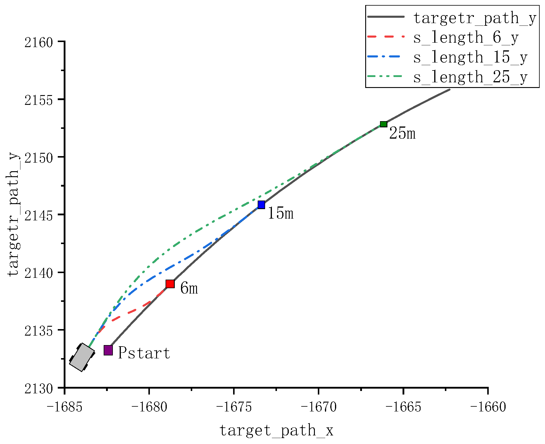
3.5.3. Clothoid Curve Length Constraint

The length of the planned control path designed by the clothoid curve is required to be long enough for two reasons. On the one hand, the algorithm proposed in this paper needs to preview a point at a distance on the clothoid curve according to the vehicle speed and the servo response delay time of the steering system. The length of the planned control path must be greater than the preview length; on the other hand, if the length of the planned control path is too short, cross error may be raised because of the large change in the curvature of the clothoid curves calculated successively. It is determined that the clothoid curve length is not less than one meter, which can achieve good tracking performance. The clothoid curve control follow path length constraint proposed in this paper is defined as follows.
{ l e n g t h ( s [ 0 ] ) > v 0.5 ( v > 2   m / s ) l e n g t h ( s [ 0 ] ) > 1.00 ( v < = 2   m / s ) ,
where l e n g t h ( s [ 0 ] ) is the length of the S[0] curve or the planned control path, and v is the current vehicle speed.

3.6. Preview Control Based on Steering System Response Hysteresis

We propose two methods to obtain the target angle of the steering wheel. The first method is to calculate the target steering angle by previewing the curvature of a point on the planned control path, as shown in the following formula.
{ κ p r e v i e w = κ v + κ v t 2 δ = tan 1 ( L κ p r e v i e w ) a n g l e = δ k ,
where κ v is the current steering curvature of the vehicle, κ is the curvature change rate of the planned control path, v is the current speed, t 2 is the steering system response hysteresis time, δ is the front wheel angle, L is the wheelbase, k is the steering system transmission ratio, κ p r e v i e w represents the target curvature of the preview, and a n g l e is the target steering angle.
The second method is to calculate the target turning rate of the steering wheel using the curvature change rate of the planned path k according to Formula (6). Then, the target angle is calculated by previewing the steering wheel angle by the steering system response hysteresis time, as shown in the following formula.
{ ω = κ k L v cos 2 ( δ v ) a n g l e = a n g l e v + ω t 2 ,
where ω is the target angular velocity of the steering wheel, δ v is the current angle of the front wheel, a n g l e v is the current steering wheel angle, and a n g l e is the target steering angle. The meaning of the other characters in Formula (14) is consistent with that in Formula (7).
The steering system response hysteresis time t2 has some differences due to the different step values of the actual target angle. If t2 is too large, the target angle may be reached in advance, resulting in tracking deviation; on the other hand, if the selection of t2 is too small, it may cause the steering response to be too slow and delay reaching the target steering angle, thus resulting in tracking deviation.

4. Test Results and Analysis

4.1. Test Method

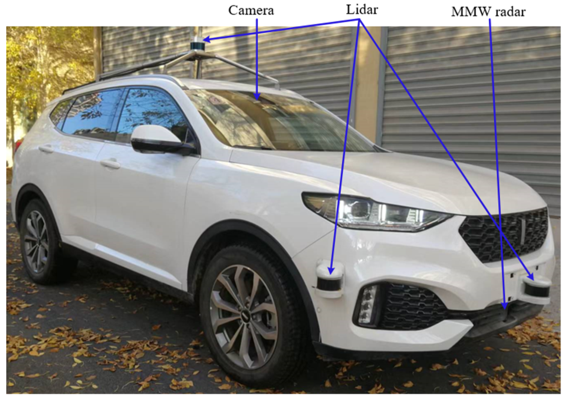
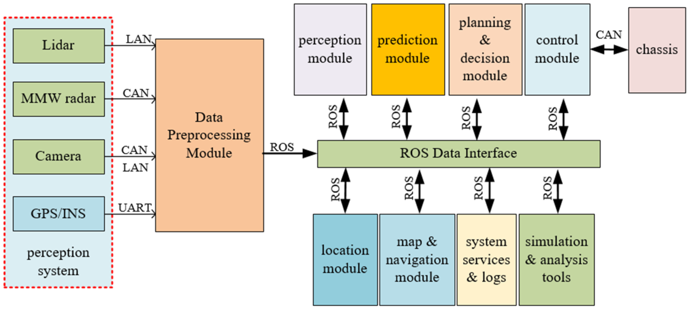
4.1.1. Test Platform

In order to verify the effectiveness of the trajectory tracking control method using the clothoid curve proposed in this paper, an intelligent vehicle modified based on Wey VV6 (as shown in Figure 5) was used for the field test. The intelligent driving software architecture used in the vehicle is shown in Figure 6, which mainly consists of a sensor system, data preprocessing module, perception module, prediction module, planning and decision-making module, positioning module, map and navigation module, control module, system service and log, simulation analysis tools, and other modules. Communication protocol interfaces are defined between modules, and data communication is carried out using the ROS platform. The platform is equipped with two Nuvo-7160GC industrial control computers, one of which is used in this experiment.

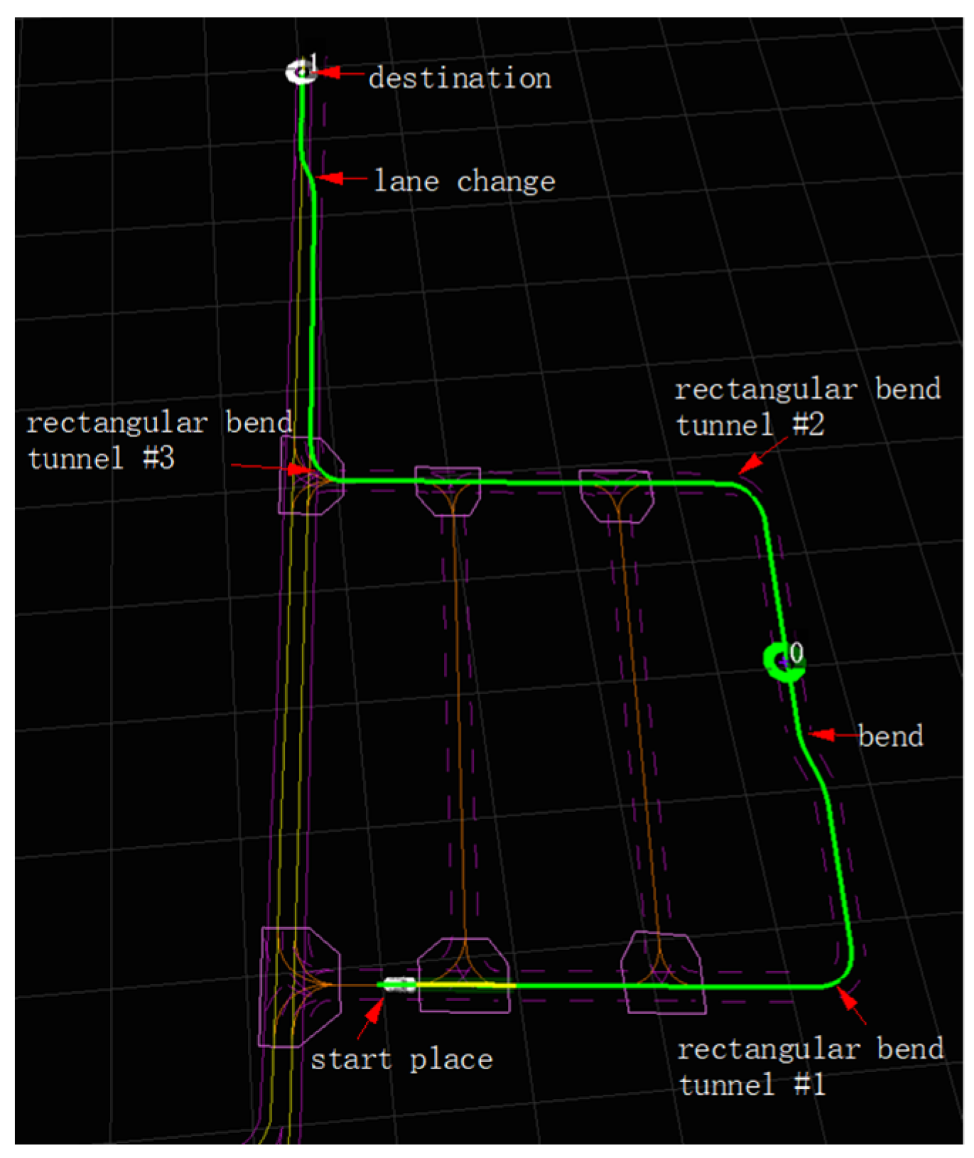
4.1.2. Test Path Design

In order to avoid the interference of misidentification and detection on the test, only differential GPS and IMU sensors were used to collect the position information in the test. The driver drove the vehicle along the set route to collect and record the positioning information of the route. Because of the differential GPS positioning system, the accuracy of the recorded path position information is ±0.02 m. When the vehicle ran in automatic mode, the decision-making module extracted the path ahead of the vehicle, calculated the position, distance, direction angle, and curvature of each path point, and sent the data to the control module in the form of a path point array. The control module used this path as the reference path to follow and calculated the control command. The control module then sent the generated control command to the drive module and forwarded it to the servo execution system via CAN messages to drive the steering wheel to execute corresponding actions. The test path is shown as Figure 7.

4.1.3. Comparison Method

The most popular geometric controllers are the pure pursuit tracking controller and the Stanley controller. Because the pure pursuit tracking controller has few parameters and is insensitive to sudden changes in the path, it is widely used in autonomous vehicles. In recent years, its optimization is mainly focused on the selection of preview points. This paper uses the pure tracking controller for comparative tests. The selection strategy of preview points adopts the method proposed in Reference [9], as shown in Formula (15). The calculation method of the front wheel target angle of the pure pursuit tracking method is shown in Equation (16) [9].
l d = { 5 v c u r < 10   kph , 0.5 v c u r 10   kph     v c u r < 50   kph , 25   50   kph   v c u r .
where l d is the preview distance, and v c u r is the current vehicle speed.
δ l d ( t ) = tan 1 ( 2 L sin ( α ( t ) ) l d ) ,
where δ l d ( t ) is the desired steering wheel angle, l d is the preview distance, L is the wheelbase, and α represents the angle between the heading angle of the vehicle and the look-ahead vector.

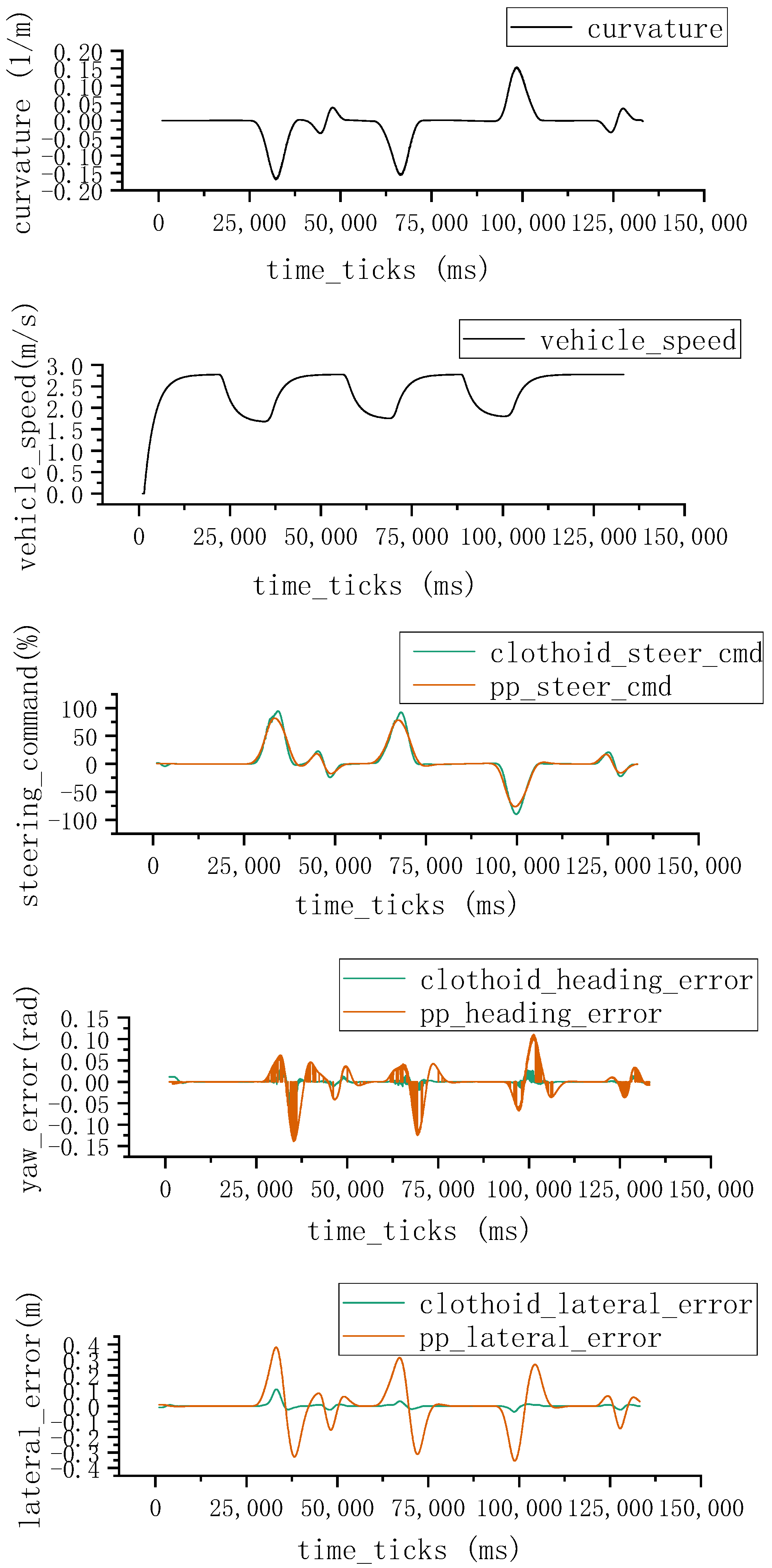
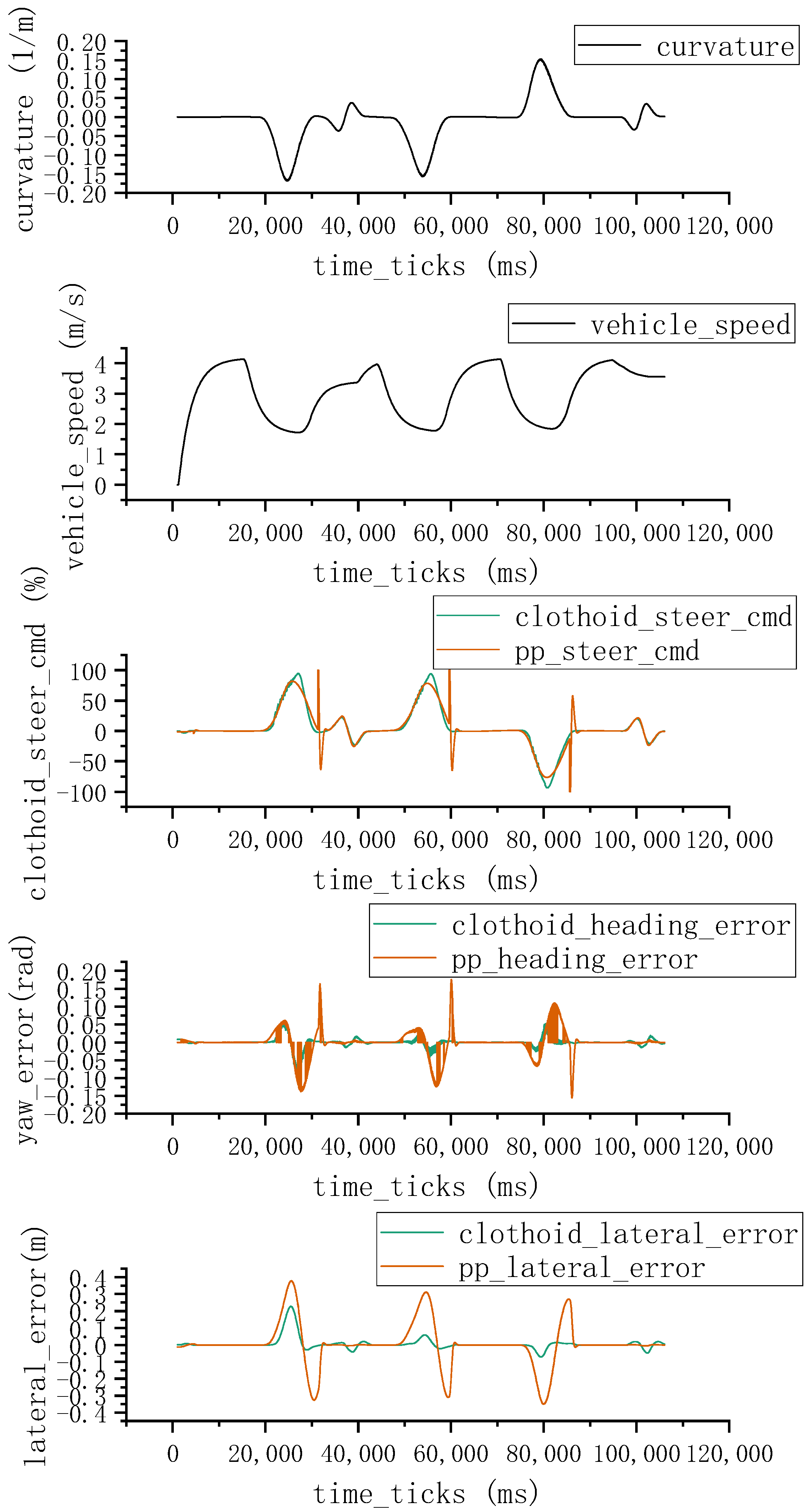
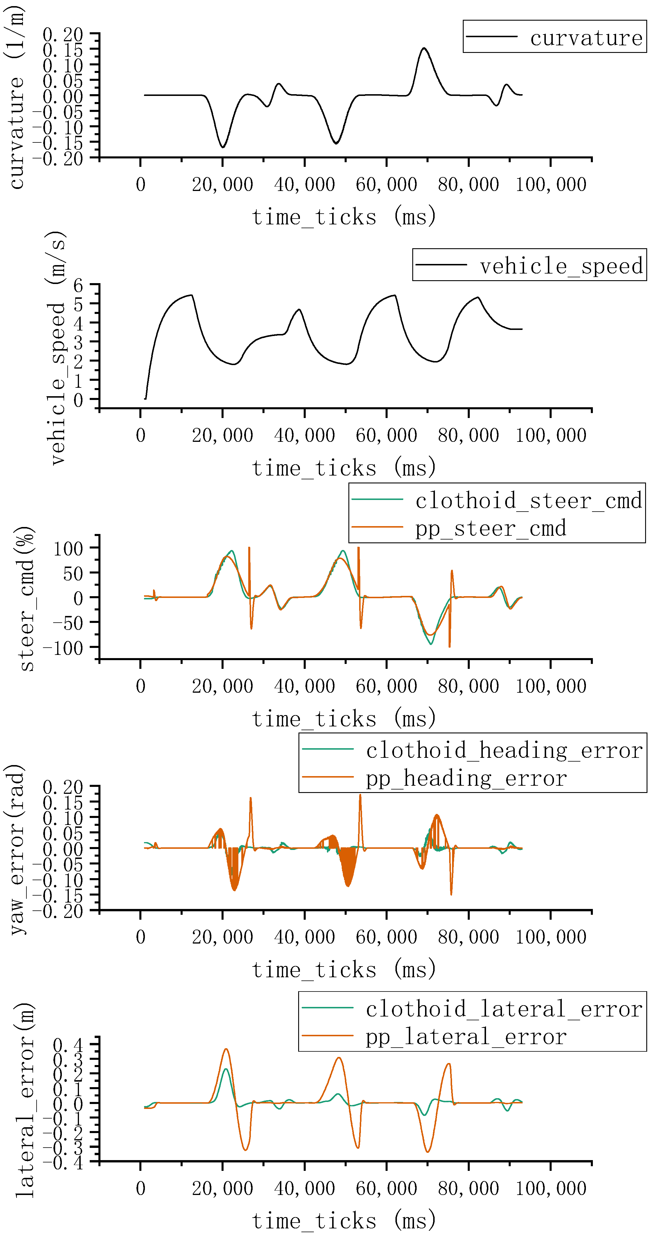
4.2. Test Results and Analysis

The performance of the trajectory tracking controller is compared and evaluated by the lateral position deviation and yaw deviation. The calculation method is as follows [22].
Maximum lateral deviation:
ε d ,   m a x = max i [ 1 N ] | ε d ,   i |
Maximum yaw deviation:
ε θ ,   m a x = max i [ 1 N ] | ε θ ,   i |
Average lateral deviation:
ε d , r m s = 1 N i = 1 N ε d , i 2 ,
Average yaw deviation:
ε θ , r m s = 1 N i = 1 N ε θ , i 2 ,
The pure pursuit method and the method proposed in this paper were tested on the designed route with speed limits of 10 km/h, 15 km/h. and 20 km/h respectively, as shown in Figure 8, Figure 9 and Figure 10. The statistics of maximum lateral deviation, maximum yaw deviation, average lateral deviation, and average yaw deviation are shown in Table 1.
The analysis of the three groups of comparative test results shows that the performance of the method proposed in this paper is generally better than the pure pursuit tracking method. In particular, the yaw deviation is improved by more than 50%. Under different speeds, both methods can control the lateral tracking deviation and yaw deviation within 5 cm on the straight track. The maximum lateral deviation and yaw deviation of both control methods occurred at the first right turn. The reason is that the maximum curvature of this turn curve is 0.168, which almost reaches the limit of the turning radius of the vehicle. The value of the steering wheel target angle output by the method proposed in this paper in this curve reaches about 94%. When the vehicle passed this curve at the speed limit of 10 km/h, due to the relatively low entry speed, the lateral deviation and heading deviation obtained at 10 km/h is less than those at the speed limits of 15 km/h and 20 km/h. During the 15 km/h and 20 km/h speed limit tests of the pure tracking method, there is a large jitter after every right turn, which leads to a large deviation in yaw. A small curvature S curve and a lane-changing scene are designed in the route. In the 10 km/h speed limit test, the performance of the method proposed in this paper is better than that of the pure pursuit tracking method. In the speed limit 15 km/h and 20 km/h tests, the tracking result of the pure tracking method is better than that of the method proposed in this paper, but the method proposed in this paper still controls the lateral tracking deviation within 5 cm. The reason for the analysis is that the preview distance of the pure pursuit tracking method is close at low speed and oscillates when tracking small curvature paths. As the speed increases, the preview distance also increases, which can better adapt to small curvature paths. However, the parameter adjustment of the method proposed in this paper requires that the speed is low enough to show better tracking performance when passing curves.
During the test, the control frequency is set to 100 HZ. Although it may require multiple calculations to solve the optimal clothoid curve in one control cycle, the method provided in Reference [18] is very efficient in solving the clothoid curve and can reach a delicate level, so the average calculation efficiency of the system can meet the real-time requirements. The system transplantation would take some work. In addition to the basic parameters of the vehicle geometric model, such as the wheelbase and the steering ratio, it is also necessary to adapt the communication delay of the control system and the response lag time parameters of the vehicle steering servo system. In general, the system has good real-time performance.

5. Conclusions

The trajectory tracking control method using a clothoid curve is proposed in this paper. First, the vehicle motion control model is constructed; then, based on the current state of the vehicle, the control system communication delay time is used to predict the vehicle state, which is the starting point of the clothoid curve. On the reference path, the optimal selection interval of the end point of the clothoid curve is selected, and finally, the optimal clothoid planned control path that satisfies the non-integrity constraints and safety conditions of vehicle driving is obtained. Based on the response hysteresis parameters of the steering system, the curvatures of points are previewed on the clothoid curve to further calculate the target angle of the output steering wheel control. A test path, including a straight lane, a right-angle turn, a curve, and lane-change scenarios, is designed in a park environment, and comparative tests are conducted against the pure pursuit tracking algorithm under the speed limits of 10 km/h, 15 km/h, and 20 km/h. The results show that the trajectory tracking control method using the clothoid curve proposed in this paper outperforms the pure pursuit tracking algorithm in terms of lateral deviation and yaw deviation indicators.
In this study, we adopted a geometric vehicle model based on Ackermann steering, so the method proposed in this paper is not applicable to the vehicle platform of other steering models, such as differential steering. At the same time, because the geometric vehicle model is used, the dynamic characteristics of the vehicle, such as the slip of the vehicle caused by the tire sideslip, are not considered. Therefore, the vehicle speed must be strictly controlled according to the curvature of the curve when turning to ensure the path tracking accuracy. In future work, we will use a different platform to test and verify the effectiveness of the method proposed in this paper and future improve the trajectory tracking performance of the method when passing curves with a small curvature.

Author Contributions

Conceptualization, J.L. (Jianshi Li) and Y.X.; methodology, J.L. (Jianshi Li) and Y.X.; software, J.L. (Jianshi Li) and S.P.; validation, J.L. (Jianshi Li), S.P. and Y.L.; formal analysis, Y.L. and J.L. (Jingtao Lou); investigation, J.L. (Jianshi Li) and J.L. (Jingtao Lou); resources, Y.X.; data curation, J.L. (Jianshi Li) and S.P.; writing—original draft preparation, J.L. (Jianshi Li) and J.L. (Jingtao Lou); writing—review and editing, Y.X., J.L. (Jingtao Lou) and Y.L.; supervision, Y.X. All authors have read and agreed to the published version of the manuscript.

Funding

This Research was funded by the military pre-research project [ZW040202]. And the APC was funded by military pre-research project.

Institutional Review Board Statement

Not applicable.

Informed Consent Statement

Not applicable.

Data Availability Statement

The data used to support the findings of this study are available from the corresponding author upon request.

Acknowledgments

The authors would like to thank the handling editor and the anonymous reviewers for their valuable comments and suggestions.

Conflicts of Interest

The authors declare no conflict of interest.

References

  1. Wang, C.; Du, Y. Lane-Changing Strategy Based on a Novel Sliding Mode Control Approach for Connected Automated Vehicles. Appl. Sci. 2022, 12, 11000. [Google Scholar] [CrossRef]
  2. Amer, N.; Zamzuri, H.; Hudha, K.; Kadir, Z.A. Modelling and Control Strategies in Path Tracking Control for Autonomous Ground Vehicles: A Review of State of the Art and Challenges. J. Intell. Robot Syst. 2017, 86, 225–254. [Google Scholar] [CrossRef]
  3. Sun, Y.; Cui, B.; Ji, F.; Wei, X.; Zhu, Y. The Full-Field Path Tracking of Agricultural Machinery Based on PSO-Enhanced Fuzzy Stanley Model. Appl. Sci. 2022, 12, 7683. [Google Scholar] [CrossRef]
  4. Li, L.; Li, J.; Zhang, S. Review article: State-of-the-art trajectory tracking of autonomous vehicles. Mech. Sci. 2021, 12, 419–432. [Google Scholar] [CrossRef]
  5. Kapania, N.; Gerdes, J. Design of a feedback-feedforward steering controller for accurate path tracking and stability at the limits of handling. Veh. Syst. Dyn. 2015, 53, 1687–1704. [Google Scholar] [CrossRef] [Green Version]
  6. Aicardi, M.; Casalino, G.; Bicchi, A.; Balestrino, A. Closed loop steering of unicycle like vehicles via Lyapunov techniques. IEEE Robot Autom. Mag. 1995, 2, 27–35. [Google Scholar] [CrossRef]
  7. Koubaa, Y.; Boukattaya, M.; Dammak, T. Adaptive Sliding-Mode Dynamic Control for Path Tracking of Nonholonomic Wheeled Mobile Robot. J. Autom. Syst. Eng. 2015, 9, 119–131. [Google Scholar]
  8. Ji, X.; He, X.; Lv, C.; Liu, Y.; Wu, J. Adaptive-neural-network-based robust lateral motion control for autonomous vehicle at driving lim-its. Control Eng. Pract. 2018, 76, 41–53. [Google Scholar] [CrossRef]
  9. Park, M.; Lee, S.; Han, W. Development of Steering Control System for Autonomous Vehicle Using Geometry-Based Path Tracking Algorithm. ETRL J. 2015, 37, 617–625. [Google Scholar] [CrossRef]
  10. Horvath, E.; Hajdu, C.; Koros, P. Novel Pure-Pursuit Trajectory Following Approaches and their Practical Applications. In Proceedings of the 2019 10th IEEE International Conference on Cognitive Infocommunications (CogInfoCom), Naples, Italy, 23–25 October 2019; IEEE: Piscataway Township, NJ, USA, 2019; pp. 597–602. [Google Scholar]
  11. Elbanhawi, M.; Simic, M.; Jazar, R. Receding horizon lateral vehicle control for pure pursuit path tracking. J. Vib. Control 2018, 24, 619–642. [Google Scholar] [CrossRef]
  12. Bertolazzi, E.; Frego, M. On the G 2 Hermite Interpolation Problem with clothoids. J. Comput. Appl. Math. 2018, 341, 99–116. [Google Scholar] [CrossRef]
  13. Krichen, M. Improving Formal Verification and Testing Techniques for Internet of Things and Smart Cities. Mobile Netw Appl. 2019, 1–12. [Google Scholar] [CrossRef]
  14. Medhat, N.; Moussa, S.M.; Badr, N.L.; Tolba, M.F. Tolba. A Framework for Continuous Regression and Integration Testing in IoT Systems Based on Deep Learning and Search-Based Techniques. IEEE 2022, 8, 215716–215726. [Google Scholar] [CrossRef]
  15. Wit, J.; Crane, C.; Armstrong, D. Autonomous ground vehicle path tracking. J. Robot. Syst. 2004, 21, 439–449. [Google Scholar] [CrossRef]
  16. Amidi, O.; Thorpe, C. Integrated Mobile Robot Control. In Proc. SPIE 1388; Mobile Robots V, 1 March 1991. [Google Scholar] [CrossRef] [Green Version]
  17. Girbés, V.; Armesto, L.; Tornero, J.; Solanes, J.E. Continuous-curvature kinematic control for path following problems. In Proceedings of the 2011 IEEE/RSJ International Conference on Intelligent Robots and Systems, San Francisco, CA, USA, 25–30 September 2011; pp. 4335–4340. [Google Scholar] [CrossRef]
  18. Shan, Y.; Yang, W.; Chen, C.; Zhou, J.; Zheng, L.; Li, B. CF-Pursuit: A Pursuit Method with a Clothoid Fitting and a Fuzzy Controller for Autono-mous Vehicles. Int. J. Adv. Robot Syst. 2015, 12, 134. [Google Scholar] [CrossRef] [Green Version]
  19. Xu, S.; Peng, H.; Tang, Y. Preview Path Tracking Control with Delay Compensation for Autonomous Vehicles. IEEE T. Intell. Transp. Syst. 2021, 22, 2979–2989. [Google Scholar] [CrossRef]
  20. Zakaria, M.; Zamzuri, H.; Mamat, R.; Amri Mazlan, S. A Path Tracking Algorithm Using Future Prediction Control with Spike Detection for an Autonomous Vehicle Robot. Int. J. Adv. Robot Syst. 2013, 10, 309. [Google Scholar] [CrossRef] [Green Version]
  21. Abd Elmoniem, A.; Osama, A.; Abdelaziz, M.; Maged, .A. A path-tracking algorithm using predictive Stanley lateral controller. Int. J. Adv. Robot Syst. 2020, 17, 172988142097485. [Google Scholar] [CrossRef]
  22. Rokonuzzaman, M.; Mohajer, N.; Nahavandi, S.; Mohamed, S. Review and performance evaluation of path tracking controllers of autonomous vehicles. IET Intell. Transp. Syst. 2021, 15, 646–670. [Google Scholar] [CrossRef]
Figure 1. Clothoid-curve-based trajectory tracking control method.
Applsci 13 02733 g001
Figure 2. Geometric model based on Ackerman steering configuration.
Applsci 13 02733 g002
Figure 3. Schematic diagram of vehicle position prediction.
Applsci 13 02733 g003
Figure 4. Influence of the selection of preview point on the calculation deviation of control path.
Applsci 13 02733 g004
Figure 5. Test platform.
Applsci 13 02733 g005
Figure 6. Software architecture.
Applsci 13 02733 g006
Figure 7. Test path.
Applsci 13 02733 g007
Figure 8. Speed limit 10 km/h trajectory tracking. Top first row: the curvatures along the field test road. Second row: actual speed of the vehicle during the trajectory tracking experiment under the speed limit of 10 km/h. It can be seen that the vehicle will slow down according to the curvature of the road ahead before entering the curve. Third row: steering wheel angle commands the comparison between the pure pursuit method and the method proposed in this paper. When tracking the curve, the method proposed in this paper increases the steering wheel angle control command later when entering the curve, and decreases the steering wheel angle control command in advance when leaving the curve, and the control amount given in the curve is also larger. It is because of this that the “cutting corner” problem suffered by the pure pursuit method is avoided. Fourth row: yaw angle deviation from the reference path point. The method proposed in this paper reduces the angle deviation to a large extent and avoids the problem of directional oscillation when turning, so as to improve the driving stability and riding comfort of the vehicle. Last row: lateral deviation from the reference path. The method proposed in this paper greatly reduces the reference path tracking error and improves the accuracy of vehicle path tracking control.
Applsci 13 02733 g008
Figure 9. Speed limit 15 km/h trajectory tracking. Top first row: the curvatures along the field test road. Second row: actual speed of the vehicle during the trajectory tracking experiment under the speed limit of 15 km/h. It can be seen that the vehicle will slow down according to the curvature of the road ahead before entering the curve. Third row: steering wheel angle commands the comparison between the pure pursuit method and the method proposed in this paper. It is noted that the steering wheel angle control commands given by the pure pursuit method suffer a drastic oscillation when leaving the right-angle turn, which does not occur in the previous test with a speed limit of 10 km/h. This problem might be caused by the improper selection of the preview distance. Fourth row: yaw angle deviation from the reference path point. The direction deviation generated by the pure pursuit tracking method when leaving the right-angle turn is actually caused by the violent oscillation of the steering wheel angle control command. Last row: lateral deviation from the reference path. Compared with the 10 km/h speed limit test, the tracking deviation of the method proposed in this paper in the first right-angle turn increased, which indicates a limitation that the trajectory tracking accuracy of the method proposed in this paper is sensitive to speed changes when passing the curve with a large curvature.
Applsci 13 02733 g009
Figure 10. Speed limit 20 km/h trajectory tracking. Top first row: the curvatures along the field test road. Second row: actual speed of the vehicle during the trajectory tracking experiment under the speed limit of 20 km/h. It can be seen that the vehicle will slow down according to the curvature of the road ahead before entering the curve. Third row: steering wheel angle commands the comparison between the pure pursuit method and the method proposed in this paper. It can be seen that the steering wheel angle control commands given by the pure pursuit method still suffer a drastic oscillation when leaving the right-angle turn. Fourth row: yaw angle deviation from the reference path point. The obvious direction deviation generated by the pure pursuit tracking method when leaving the right-angle turn also appears as expected. Last row: lateral deviation from the reference path. The performance of the method proposed in this paper is obviously better than the pure pursuit tracking method when passing through right-angle curves, but the accuracy is slightly lower when passing through S curves with a small curvature.
Applsci 13 02733 g010
Table 1. Test result statistics. Clothoid represents the trajectory tracking control method based on the clothoid curve proposed in this paper. PP represents the pure pursuit tracking method.
Limited Speed
(km/h)
ε d , m a x   ( m ) ε θ , m a x   ( rad ) ε d , r m s   ( m ) ε θ , r m s   ( rad )
ClothoidPPClothoidPPClothoidPPClothoidPP
100.1090.3810.05570.13900.01570.12250.00710.03148
150.2270.3780.09340.17530.03650.12180.01340.03662
200.2320.3680.08640.17270.03930.12310.01400.03754
Disclaimer/Publisher’s Note: The statements, opinions and data contained in all publications are solely those of the individual author(s) and contributor(s) and not of MDPI and/or the editor(s). MDPI and/or the editor(s) disclaim responsibility for any injury to people or property resulting from any ideas, methods, instructions or products referred to in the content.

