Study on Shock Initiation Randomness of Energetic Materials on a Macroscopic Scale

Abstract

The shock initiation randomness problem of energetic materials (SIREM) is an important problem in the research field of energetic material safety. With the purposes of solving SIREM on a macroscopic scale and obtaining the statistics, such as the initiation probabilities of energetic materials and the statistical characteristics of the detonation pressure, this paper considers the effect of the randomness of the parameters of the Lee–Tarver equation of reaction rate and the JWL equation of state of energetic materials and the randomness of load intensity parameters—such as fragment shock velocity—on the randomness of the shock initiations of energetic materials. It then decomposes SIREM into an initiation probability problem (IP) and a detonation pressure randomness problem (DPR). Further, with the Back Propagation Neural Networks optimized by the Genetic Algorithm (GABPNN) as the surrogate models of the numerical models of two-phase reactive flow, this paper proposes the approach of solving IP and DPR in turn, adopting Monte Carlo Simulations, which use the calculations of GABPNNs as repeated sampling tests (GABP-MCSs). Finally, by taking the shock initiation randomness problem of Composition B as an applied example, this paper adopts GABP-MCS under the randomness conditions that the means of fragment shock velocities are 1050 m/s and 1000 m/s and that the coefficients of variation (CVs) of BRVs are 0.005, 0.01, 0.015, and 0.02 in order to obtain the initiation probabilities of Composition B and the statistical characteristics, such as the means and CVs of the detonation pressure. It further observes the variation tendencies that these statistics show under various randomness conditions, so as to prove the effectiveness of GABP-MCS in solving SIREM. Therefore, this paper investigates SIREM on a macroscopic scale and proposes a universal technique for solving SIREM by GABP-MCS, in the hope of shedding some light on the SIREM study.

1. Introduction

Energetic materials, with randomly distributed micro-sized grains and many voids and cracks among them, are heterogeneous on a mesoscopic scale and show stochastic detonation characteristics on a macroscopic scale. Thus, the macro responses of energetic materials are generally stochastic under the action of shock loads. This explains why the shock load indexes of the initiation probability 50% (such as the fragment shock velocity, drop hammer height, shock pressure, or shock energy) are always the important characteristic indexes of the impact sensitivity tests of energetic materials [1,2,3,4]. Gresshoff [5] earlier recognized the importance of solving the shock initiation randomness problem of energetic materials (SIREM) and established the Probabilistic Shock Threshold Criterion based on the James Initiation Criterion and the assumption of initiation probability distribution, but they also contended that these empirical criterions, such as the James Initiation Criterion, were more crude than the numerical simulations using reactive flow models in determining the impact responses of energetic materials. Similarly, Rashkovskii [6] constructed a probabilistic model of the shock initiation of heterogeneous explosive materials based on the critical initiation stress of explosive grains and the assumption of initiation probability distribution. In recent years, with the continuously improved mesoscale numerical simulation techniques, many research teams have begun to apply the numerical models of multiphase reactive flow in the SIREM study at mesoscale. Baer [7] took the initiative and adopted the mesoscale numerical model of multiphase reactive flow to solve SIREM, and they developed a universal method to describe the ignition randomness of energetic materials at mesoscale. After that, the research team of Zhou also carried out in-depth and comprehensive studies on SIREM by adopting the mesoscale numerical models of multiphase reactive flow. Zhou [8,9] developed an approach to computationally predict and quantify the stochasticity of the ignition process in condensed explosives under shock loads and studied the effect of the microstructure randomness on the shock response randomness of condensed explosives. Zhou [10,11,12] also developed an approach to calculate the probabilistic ignition threshold of condensed explosives based on mesoscale numerical simulation techniques and empirical ignition criterions. Zhou [13] also used this approach and the newly developed probabilistic formulation to calculate the probabilistic ignition thresholds of the HMXs with four microstructural forms. Zhou [14] also used three-dimensional, mesoscale, numerical simulation techniques to calculate the run-to-detonation distances of condensed explosives and led to the probabilistic formulations for the run-to-detonation distances as the shock pressure functions. In addition to Zhou’s team, other research teams also used the mesoscale numerical models of multiphase reactive flow to solve SIREM. Kittell [15] believed that the microstructure randomness of heterogeneous energetic materials could lead to the randomness of heat release rates from a chemical reaction, and that the heat release fluctuations of heterogeneous energetic materials could be coupled to the reactive Euler equations, which could then be solved via the Riemann problem. Based on the study results in the literature [15], Kittell [16] drew the conclusion that the randomness of the heat release, yield strength, and material impedance could also lead to the reaction rate randomness of heterogeneous solid explosives, and constructed the stochastic burn model of heterogeneous solid explosives by using Langevin-type equations. Lee [17] considered the randomness of the specific heat, Grüneisen parameter, bulk modulus, yield strength, thermal expansion coefficient, and thermal conductivity of HMXs at mesoscale and established the probability density function of the run-to-detonation distances of HMXs by applying the Meso-informed Ignition and Growth model. Bakarjia [18] treated the initial porosity in the microstructure of energetic materials as a random field and adopted the Monte Carlo Simulations of a two-phase, five-equation, dynamic compaction model to calculate the probability of hotspot initiation. Mi [19] investigated the influence of the randomness of four microbubble distributions on the impact sensitivity randomness of liquid nitromethane by the mesoscale numerical simulation technique. Liu [20] researched the mechanical–thermal–chemical response of PBXs under low-velocity impact, obtained the influence of the density number and the statistical distribution of microcracks on the impact ignition of PBXs, and described the ignition probability of PBXs based on the Weibull distribution. Miller [21] proposed a simplified shock initiation criterion, classified the initiation responses of HMXs under different test conditions by using mesoscale numerical simulations, and obtained the probabilistic responses of the HMX samples to the variations in the mean porosity and chemical kinetics rate.

It can be seen from the researches above that SIREM is a common problem in the research field of energetic material safety, which has been solved, under the assumption of initiation probability distribution, by applying various techniques, such as empirical initiation criterions and mesoscale numerical simulations of multiphase reactive flow, with substantial achievements. However, none of the research has used the numerical models of multiphase reactive flow in solving SIREM on a macroscopic scale. Therefore, the initiation probabilities of energetic materials with standard specifications under standard test conditions and, thus, their probabilistic initiation thresholds can be obtained through the previous research results. So is the effect of the microstructure randomness on the shock sensitivity randomness of the energetic material specimens. Yet, unknown remain the initiation probabilities of the energetic materials under complex working conditions (such as complex structural shielding, shock loads, and geometrical shapes) and the randomness of the detonation pressure in different positions inside these energetic materials after they are initiated. This means that the existing research has conducted only a preliminary theoretical study on SIREM and that it is difficult to be widely applied to engineering practices, such as assessments of the shock safety randomness of ammo and rocket motors. In this sense, it is necessary to analyze SIREM on a macroscopic scale and to apply the macroscale numerical models of multiphase reactive flow and their surrogate models in the SIREM study in the hope of better meeting the needs of engineering practices.

Some research has provided reference to analyzing SIREM on a macroscopic scale. Gresshoff [5] argued that the Lee–Tarver equation of reaction rate was tuned to an idealized 50% threshold and, thus, could not directly provide the analyst with a sense of “margin to initiation”; Gresshoff [5] also pointed out that uncertainties from experimental conditions and random heterogeneities in the specimens could lead to the randomness of the shock initiation test results of energetic materials. Landerville [22] showed that the parameters vary to a large degree among experiments due to the inherent noise of experiments and the inconsistencies in fitting ranges and schemes. In addition, in studying the randomness of underwater explosions, the research team of Chen contended that the parameters of the Jones–Wilkins–Lee (JWL) equation of state of energetic materials, obtained from parametric measurement tests, demonstrated a random nature, which led to the randomness of the detonation pressure of energetic materials [23]. In their study of the stochastic dynamics of structures under explosive loads, they also argued that the parameters of the Mie–Gruneisen equation of state, the Johnson–Cook constitutive equation, and the Johnson–Cook failure model of metal structures showed randomness, which led to the randomness of the normal stress and deviatoric stress of metal structures under explosive loads, and further led to the randomness of the dynamic responses of metal structures [24,25]. Enlightened by these researches, it is natural to hold that the parameters of the Lee–Tarver equation of reaction rate and the JWL equation of state will probably show random errors in parametric measurement tests. Since, in the numerical models of two-phase reactive flow, the Lee–Tarver equation of reaction rate describes the reaction rates of energetic materials, and the JWL equation of state describes the Pressure–Volume–Energy (P-V-E) relationships of energetic materials, the parameters of these two equations can fully describe the detonation characteristics of energetic materials. Therefore, when solving SIREM on a macroscopic scale by adopting the numerical models of two-phase reactive flow and their surrogate models, they should attribute the randomness of SIREM to the randomness of the parameters of these two equations and the randomness of the physical quantities, such as the fragment shock velocity that affects shock load intensity, which should be taken as the starting point to further study the initiation probabilities of energetic materials under random shock loads and the randomness of the detonation pressure after energetic materials are initiated. In fact, the randomness of the parameters of these two equations is the macroscopic manifestation of the randomness of the microstructure of energetic materials considered in the literature [7,8,9,10,11,12,13,14,15,16,17,18,19,20,21]; hence, these two kinds of randomness are equivalent and can both represent the randomness of the detonation characteristics of energetic materials, which will be also mentioned in Discussion 5.

In addition, since the numerical models of two-phase reactive flow involve the processes in which the unreacted energetic materials of the condensed phase are transformed into the reaction products of gas phase, a very complicated relationship appears between the parameter randomness of the Lee–Tarver equation of reaction rate and the JWL equation of state and the shock response randomness of energetic materials, and also marked differences appear in the random response values between the initiation and non-initiation states of energetic materials. This means that the common stochastic analysis methods, such as semi-analytical methods and surrogate model methods of response surfaces, may not be used to solve SIREM on a macroscopic scale. Therefore, what should be adopted are the methods of combining the Artificial Neural Networks (ANNs), which are more powerful in nonlinear mapping, with Monte Carlo Simulations (MCSs) to solve SIREM on a macroscopic scale. Since the Back Propagation Neural Network optimized by the Genetic Algorithm (GABPNN) is an ANN with strong nonlinear mapping ability [26,27,28,29], this paper adopts GABPNNs as the surrogate models of the numerical models of two-phase reactive flow, and it adopts the MCSs, which use the calculations of GABPNNs as repeated sampling tests (GABP-MCS) to solve SIREM. The specific reasons for selecting GABP-MCS will be given in Discussion 5.

In a nutshell, in order to develop a universal technique for calculating the initiation probabilities of energetic materials under complex working conditions and the statistical characteristics of detonation pressure, so as to make the study on SIREM better meet the needs of engineering practices, this paper investigates SIREM on a macroscopic scale, decomposes SIREM into an initiation probability problem (IP) and a detonation pressure randomness problem (DPR), and identifies the basic random variables (BRVs) and random responses (RRs) of IP and DPR. Then, this paper proposes the approaches of adopting GABP-MCS to solve IP and DPR in turn. Finally, by taking the shock initiation randomness problem of Composition B as an example, this paper demonstrates the specific process of adopting GABP-MCS to solve SIREM and verifies the effectiveness of this integrated method, in the hope of providing a technical reference for further study on SIREM.

2. Problem Analysis

2.1. Problem Decomposition

Under the effects of both the detonation characteristic randomness of energetic materials and the shock load randomness, it is a random problem whether energetic materials can be initiated. So is the detonation pressure after energetic materials are initiated. Therefore, the SIREM study on a macroscopic scale should process the initiation probabilities of energetic materials and the randomness of detonation pressure after energetic materials are initiated in turn. It is necessary to decompose SIREM into an initiation probability problem (IP) and a detonation pressure randomness problem (DPR).

2.2. BRVs of the Problem

Since the randomness of the shock initiation of energetic materials is caused by the randomness of the detonation characteristics of energetic materials and the randomness of shock load conditions, the BRVs of SIREM should also be divided into the BRVs on the detonation characteristics of energetic materials and the BRVs on shock load conditions. The following is the identification of these two kinds of BRVs.

(1)

BRVs on detonation characteristics of energetic materials

In the numerical models of two-phase reactive flow of the shock initiation problem of energetic materials, the equations of reaction rate, showing the shock initiation reaction rate of energetic materials, generally adopt the Lee–Tarver equation of reaction rate, and the equations of state of the unreacted energetic materials of the condensed phase and the reaction products of the gas phase generally adopt the JWL equation of state. See the two in Equations (1) and (2) [30,31,32].

$$\frac{d\lambda }{dt}=I{\left(1-\lambda \right)}^b{\left(\mu -a\right)}^x+G_1{\left(1-\lambda \right)}^c{\lambda }^d{p}^y+G_2{\left(1-\lambda \right)}^e{\lambda }^g{p}^z$$

(1)

where λ is the fraction of an energetic material that has reacted, t is the time,$\frac{d\lambda }{dt}$ is the reaction rate, μ is the current compression degree, a is the critical compression degree, and I, b, x, G₁, c, d, y, G₂, e, g, and z are the parameters.

$$p=A\left(1-\frac{w}{R_{1}V}\right)\exp \left(-R_{1}V\right)+B\left(1-\frac{w}{R_{2}V}\right)\exp \left(-R_{2}V\right)+\frac{wE}{V}$$

(2)

where p is the pressure, V is the relative volume, E is the energy in per unit volume, and A, B, R₁, R₂, and w are the parameters. The five parameters of unreacted energetic materials and reaction products are respectively marked as A_c, B_c, R_c1, R_c2, w_c, and A_g, B_g, R_g1, R_g2, w_g in order to distinguish between the two types.

The literature [32] has pointed out that the three terms in the Lee–Tarver equation of reaction rate are the ignition term, growth term, and completion term. For the parameters of these three terms, a controls the critical compression degrees of energetic materials, and when μ is less than a, energetic materials cannot be initiated; I, G₁, and G₂ are the coefficients of these three terms; b, c, d, e, and g are the burnup indices of these three terms; y and z are the pressure indices of the growth term and completion term; I and x control the number of hot spots; b and c control the combustion of inward spherical particles; G₁ and d control the reaction growth duration at the early stage of hot spots; and G₂ and z control the reaction rate at high pressure. For the parameters of the JWL equation of state, A_c, B_c, A_g, and B_g are the parameters of the linear relationship between the detonation pressure and the isentropic expansion pressure, and R_c1, R_c2, w_c, R_g1, R_g2, and w_g are the parameters related to energetic materials. Therefore, the parameters of these two equations can fully describe the detonation characteristics of energetic materials, and the effect of the changes of the factors, such as the density, temperature, and humidity, on the detonation characteristics of energetic materials can also be expressed by the numerical changes of these parameters. In addition, the parameters of the Lee–Tarver equation of reaction rate are fitted by the shock initiation tests and numerical simulations [33,34,35], and the parameters of the JWL equation of state are fitted by the cylinder tests and numerical simulations [36,37,38]. The literature [5,22,23,24,25] suggests that such parametric measurement tests and corresponding numerical simulations generally have random errors, and so do the parameters obtained. Based on the previous achievements, this paper holds that the parameters of these two equations also have randomness, and the randomness of the detonation characteristics of energetic materials can also be described by the randomness of these parameters. Therefore, the main BRVs on the detonation characteristics of energetic materials can be selected from these parameters, and the randomness of the factors, such as the density, temperature, and humidity of energetic materials, can also be expressed by the randomness of these parameters. In addition, the relationship between the randomness of these parameters and the randomness of the microstructure of energetic materials considered in the literature [7,8,9,10,11,12,13,14,15,16,17,18,19,20,21] will be discussed in Discussion 5.

(2)

BRVs on shock load conditions

Since the mass m, shock velocity v, and shock angle θ of a fragment are the important physical quantities that directly affect the intensity of shock loads, the randomness of shock load conditions can be represented by the randomness of these physical quantities. Therefore, the main BRVs on shock load conditions can be selected from these physical quantities.

2.3. RRs of the Problem

Since SIREM is decomposed into IP and DPR, the RRs of IP and DPR should be identified respectively.

(1)

RR of IP

In IP, the initiation-recognizing coefficient δ as a new physical quantity is introduced to recognize whether energetic materials are initiated under the combined action of the above two kinds of BRVs; that is, if energetic materials are initiated, δ will be recognized to be 1, and if not, δ will be recognized to be 0. So, under the action of BRVs, the randomness of the shock initiation of energetic materials can be represented by the randomness of the 0–1 recognition results of δ. In this sense, δ should be defined as the RR of IP, and IP can be summarized as the problem of calculating the initiation probabilities R’s of energetic materials under the action of BRVs, according to the statistical analysis results of δ.

(2)

RR of DPR

In DPR, the detonation pressure P of energetic materials should be defined as the RR of DPR, and DPR can be summarized as the problem of calculating the statistical analysis results of P under the combined action of the above two kinds of BRVs.

Above is the analysis of SIREM on a macroscopic scale. Figure 1 below is the corresponding flow chart.

It should be noted that the above BRVs are just those that may be involved in SIREM on a macroscopic scale. Yet, in studies, it is necessary to take real factors into account in order to identify with caution the main BRVs involved and to obtain their actual statistical distributions.

3. Methodology

Since the principles of GABPNN have been discussed in a lot of literature [26,27,28,29], the following will present directly the main processes of using GABP-MCS to solve SIREM on a macroscopic scale, and the reasons for selecting this method will be given in Discussion 5.

(1)

Constructing training sample sets and test sample sets

Firstly, BRV sample points are randomly generated according to the statistical distributions of BRVs, and the repeated numerical simulations are conducted based on the numerical models of two-phase reactive flow, so as to obtain the 0–1 recognition result of δ and the P of each gauge in numerical models that correspond to each BRV sample point. Then, these data are standardized, and the standardized BRV sample points are taken as the input data, and the 0–1 recognition results of δ are taken as the expected output data, so as to construct the training sample sets and test sample sets of the GABPNN of IP. Finally, the standardized BRV sample points that can lead energetic materials to be initiated are selected from all the standardized BRV sample points and are taken as the input data, and the standardized values of the P of each gauge are taken as the expected output data, so as to construct the training sample sets and test sample sets of the GABPNN of DPR.

In addition, it should be pointed out that, in the repeated numerical simulations, whether detonation waves are generated inside energetic materials under shock loads can be taken as the shock initiation criterion of energetic materials. That is, if detonation waves are generated, it means energetic materials are initiated, and δ is assigned as 1. If no detonation wave is generated, it means energetic material are not initiated, and δ is assigned as 0.

(2)

Constructing surrogate models of IP and DPR

Two GABPNNs are trained and tested by the training sample sets and test sample sets of IP and DPR, respectively, so as to construct the surrogate models of IP and DPR. Furthermore, IP is a problem of pattern classification, and there is a very complicated mapping between BRVs and δ, so the double-hidden-layer GABPNN should be chosen as the surrogate model of IP. DPR is a function approximation problem. Cotter [39] and Castro [40] have proven that the forward artificial neural networks of a 3-layer structure can address most function approximation problems, so the single-hidden-layer GABPNN can be taken as the surrogate model of DPR.

(3)

Addressing IP and DPR by GABP-MCSs

Firstly, new BRV sample points are generated, which conform to the corresponding statistical distribution and whose sampling ranges and densities meet statistical needs, and these BRV sample points are standardized, so as to construct the prediction sample sets of IP. Then, all the standardized BRV sample points of the prediction sample sets of IP, as input data, are inputted in turn into the surrogate model (GABPNN) of IP, so as to quickly calculate the 0–1 recognition results of δ corresponding to these sample points. Then, these 0–1 recognition results of δ are statistically analyzed, so as to obtain the estimates of the R’s of energetic materials, thus solving IP.

After that, according to the above 0–1 recognition results of δ, the standardized BRV sample points that can lead energetic materials to be initiated are selected from the prediction sample sets of IP, so as to constitute the prediction sample sets of DPR. Then, all the standardized BRV sample points of the prediction sample sets of DPR, as input data, are inputted in turn into the surrogate model (GABPNN) of DPR, so as to quickly calculate the output results corresponding to these sample points. Then, these output results are inversely standardized, so as to obtain the predicted values of the P of each gauge in numerical models corresponding to these sample points. Finally, the predicted values of the P of each gauge are statistically analyzed, so as to obtain the estimates of the statistical characteristics, such as the mean and coefficient of variation (CV) of the P of each gauge, thus solving DPR.

The above processes are shown in the global technical route in Figure 2.

4. Applied Example

Composition B, composed of TNT and RDX in fixed proportions, which are typical energetic materials, and they are widely used as military explosives. Similar to most energetic materials, the shock initiation of Composition B can also be simulated by the numerical models of two-phase reactive flow, and the shock initiation reaction rate and P-V-E relationship of Composition B can also be described by the Lee–Tarver equation of reaction rate and the JWL equation of state, respectively. Therefore, Composition B is representative among various kinds of energetic materials. It can also be used as an example of solving SIREM on a macroscopic scale with the specific processes of adopting GABP-MCS to solve the shock initiation randomness problem of Composition B. Therefore, the shock initiation test of Composition B with shield plate recorded in the literature [41] is taken as the applied example in this paper, and the exploration of the randomness in this example will be expressed in detail to demonstrate the specific processes of solving SIREM by GABP-MCS and to verify the effectiveness of this integrated method. In addition, as the Back Propagation Neural Networks (BPNN) and Radial Basis Function Neural Network (RBFNN) are two very classical ANNs, they are usually used as the comparisons of other ANNs. Therefore, in this example, these two ANNs are also used as the comparisons of GABPNN, so as to investigate the advantages of GABPNN as the surrogate model of the numerical model of two-phase reactive flow.

4.1. Numerical Model

The example [41] took Composition B as the test explosives, the 5 mm-thick steel plates as the shield plates, and the 20 mm-long cylindrical steel with a diameter of 10 mm as the fragments. The test results showed that, with a shock velocity of fragments lower than 1003.5 m/s, Composition B was not initiated, while with a shock velocity of fragments higher than 1049.8 m/s, Composition B was initiated. It can, thus, be seen that the critical shock initiation velocity of Composition B should be between 1000 m/s and 1050 m/s under the above working conditions.

In the repeated numerical simulations of the randomness study on this example, the numerical model of two-phase reactive flow worked as the theoretical model, the generalized interpolation material point method (GIMPM) [42] worked as the numerical simulation method, and the calculation program was the self-compiled GIMPM program in the Fortran language. The numerical model constructed by this GIMPM program is shown in Figure 3, and the coordinates of the three gauges in this model are shown in

Table 1. The coordinates of the gauges.

Gauge Number	1	2	3
x coordinate (cm)	15.0	19.0	19.0
y coordinate (cm)	3.0	0.0	3.0

. In addition, the deterministic parameter values of Composition B in the Lee–Tarver equation of reaction rate and the JWL equation of state were taken from the literature [43], and these deterministic parameter values are shown in

Table 2. The deterministic parameter values of Composition B in the Lee–Tarver equation of reaction rate.

Parameter	a	I (μs−1)	b	x	G1 (Mbar−yμs−1)	c	d	y	G2 (Mbar−zμs−1)	e	g	z
Value	0.01	44.0	2/9	4.0	414.0	2/9	2/3	2.0	0.0	0.0	0.0	0.0

and

Table 3. The deterministic parameter values of Composition B in the JWL equation of state.

Parameter	Ac (Mbar)	Bc (Mbar)	Rc1	Rc2	wc	Ag (Mbar)	Bg (Mbar)	Rg1	Rg2	wg
Value	778.1	−0.05031	11.3	1.13	0.8938	5.242	0.07678	4.2	1.1	0.34

.

For the accuracy of the training sample sets and the test sample sets constructed by the GIMPM program, it is necessary to verify in advance the accuracy of the test result simulations of this example under this program. To this end, this program simulates the shock response results of Composition B under the shock load conditions that the fragment impact velocities are 1003.5 m/s and 1049.8 m/s, respectively. The pressure curves of the three gauges are shown in Figure 4 and the color contour plots of the pressure in Figure 5.

Figure 4 and Figure 5 show that when the fragment shock velocity is 1049.8 m/s, all the pressure peaks of the three gauges are over 20 GPa, and detonation waves are also generated inside Composition B, suggesting that Composition B has been initiated by the shock load. What can also be concluded is that when the fragment shock velocity is 1003.5 m/s, the pressure curves of the three gauges are all gentle, with a pressure peak lower than 2.5 GPa, and stress waves with low pressure, not detonation waves, are generated inside Composition B, suggesting that Composition B has not been initiated by the shock load. These numerical simulation results are consistent with the test results. Thus, this program can accurately simulate the shock initiation of Composition B, and the training sample sets and test sample sets constructed by the repeated numerical simulations via this program can also be identified as accurate and qualified to meet the needs of training and testing the GABPNNs.

4.2. Identification of BRVs and RRs

In this example, each test used cylindrical steel fragments of the same size, and the ballistic trajectories of all the fragments were horizontal straight lines; so, the randomness of the masses m and the shock angles θ of these fragments could be ignored. However, due to the significant influence of the charge errors of the fragment shooting gun and the fragment shock velocity recording errors of the recording equipment, the fragment shock velocity v recorded in each test had obvious randomness. In addition, according to Table 2, the values of all 4 parameters, G₂, e, g, and z, are 0.0, which indicates that the Lee–Tarver equation of reaction rate of Composition B does not have the completion term. So, in this example, there are 19 main BRVs, namely, the 8 parameters a, I, b, x, G₁, c, d, and y in the ignition and the growth terms of the Lee–Tarver equation of reaction rate, and the 10 parameters A_c, B_c, R_c1, R_c2, w_c, A_g, B_g, R_g1, R_g2, and w_g in the JWL equation of state, and the v in the shock load conditions. The RRs in the IP and DPR are, respectively, the δ and the P’s of the three gauges in the numerical model shown in Figure 3 and Table 1.

4.3. Randomness Study

For conciseness and brevity of expression, the shock initiation randomness problem of Composition B is also abbreviated to SIREM in this example. According to what has been discussed in Section 4.1, when the mean $\overline{v}$ of the v is 1050 m/s or 1000 m/s, Composition B approaches the critical shock initiation state, with obvious randomness in the shock initiation, so the SIREM was solved under the two shock load conditions where the values of the $\overline{v}$ were, respectively, 1050 m/s and 1000 m/s. Moreover, in order to reveal the common and universal aspects of the SIREM study, it is assumed that the 19 main BRVs in this example are all independent of each other and subject to the normal distribution, and the 4 randomness conditions, in which the CVs of these BRVs were, respectively, 0.005, 0.01, 0.015, and 0.02, were considered under these 2 shock load conditions.

4.3.1. Shock Load Condition Where $\overline{v}$ Is 1050 m/s

(1)

Study on IP

(i) Constructing training sample set and test sample sets

In addressing the IP when the $\overline{v}$ is 1050 m/s, in order to guarantee the excellent generalization ability of the ANNs, 2000 sample points were generated for the BRVs with the CV of 0.02, and 500 sample points were generated for the BRVs with the CV of 0.005, so as to construct the training sample set with 2500 sample points. Then, a test sample set of 1000 sample points was constructed for the BRVs with each of the CVs of 0.005, 0.01, 0.015, and 0.02. The four test sample sets tested whether the ANNs could accurately calculate the RRs under these randomness conditions. The statistical results of the initiation and non-initiation frequencies of Composition B in these training sample set and test sample sets are shown in

Table 4. The statistical results of the initiation and non-initiation frequencies of Composition B in the training sample set and test sample sets under the shock load condition where $\overline{v}$ is 1050 m/s.

Sample Set		Sample Size q	Initiation Frequency	Non-Initiation Frequency
Training sample set		2500	1554	946
Test sample set	CV of BRVs being 0.005	1000	768	232
	CV of BRVs being 0.01	1000	685	315
	CV of BRVs being 0.015	1000	612	388
	CV of BRVs being 0.02	1000	585	415

.

(ii) Determining the structure and important parameters of ANNs

In this example, according to the numbers of the BRVs and RR in the IP, the neuron numbers of the input layer, first hidden layer, second hidden layer, and output layer of the GABPNN for the IP were, respectively, set as 19, 25, 15, and 1. So, the structure of this GABPNN was $19\times 25\times 15\times 1$. In addition, the network maximum training time T_max was set as 20,000, the network training rate R_t was set as 0.05, the network training allowable error E_a was set as 0.001, the population size M_p was set as 20, the maximum generation G_max was set as 30, the chromosome crossover probability P_c was set as 0.75, the chromosome mutation probability P_m was set as 0.1, and the fitness coefficient C was set as 20.0.

In addition, the structure and corresponding parameters of the BPNN were the same as the corresponding ones of the GABPNN. The neuron numbers of the input layer and output layer of the RBFNN were the same as the corresponding ones of the GABPNN, and the neuron number of the hidden layer of the RBFNN was equal to the sample size q of the training sample set.

(iii) Performance comparison of ANNs

Firstly, the GABPNN, BPNN, and RBFNN were trained by the above training sample set. Then, these three trained ANNs were tested by each of the above four test sample sets, with the test results shown in

Table 5. The comparison of the test results of the ANNs in the IP study under the shock load condition where $\overline{v}$ is 1050 m/s.

Test Sample Set		ANN Being Tested	δT Being the Same as δE		δT Being Different from δE		Accuracy of Testing (%)
CV of BRVs	Test Number		Both δT and δE Being 1	Both δT and δE Being 0	δT Being 1 and δE Being 0	δT Being 0 and δE Being 1
0.005	1000	GABPNN	723	180	52	45	90.3
		BPNN	697	145	87	71	84.2
		RBFNN	746	102	130	22	84.8
0.01	1000	GABPNN	627	275	40	58	90.2
		BPNN	611	269	46	74	88.0
		RBFNN	663	238	77	22	90.1
0.015	1000	GABPNN	564	358	30	48	92.2
		BPNN	548	349	39	64	89.7
		RBFNN	589	331	57	23	92.0
0.02	1000	GABPNN	553	379	36	32	93.2
		BPNN	536	375	40	49	91.1
		RBFNN	561	359	56	24	92.0

and Figure 6. In Table 5, the δ_T stands for the calculation results of these three ANNs (the actual output results of the δ), and the δ_E the expected output results of the δ.

According to the test results shown in Table 5 and Figure 6, all the test accuracy results with which the GABPNN calculated the 0–1 recognition results of the δ corresponding to these 4 test sample sets were above 90%, and these test results were also better than the test results of BPNN and RBFNN. It is proved that the GABPNN has stronger nonlinear mapping ability than the BPNN and RBFNN, and the GABPNN can accurately calculate the 0–1 recognition results of the δ corresponding to the BRV sample points. Therefore, the GABPNN can be used as the surrogate model of the IP, and the GABP-MCS can also be used to estimate the R’s of Composition B.

(iv) Estimation of R based on GABP-MCS

A prediction sample set with 100,000 sample points was constructed under each of the above 4 randomness conditions, and the 0–1 recognition results of the δ corresponding to these 4 prediction sample sets were obtained by the GABP-MCS, so as to obtain accurate estimates of the actual R’s of Composition B under these 4 randomness conditions. The results are shown in

Table 6. The calculation results of the GABP-MCS in the IP study under the shock load condition where $\overline{v}$ is 1050 m/s.

CV of BRVs	Simulation Number	Initiation Frequency	Non-Initiation Frequency	R (%)
0.005	100,000	78,654	21,346	78.65
0.01	100,000	66,291	33,709	66.29
0.015	100,000	61,281	38,719	61.28
0.02	100,000	58,711	41,289	58.71

and Figure 7.

According to the statistical data in Table 6 and the correlation curve in Figure 7, it can be concluded that when the $\overline{v}$ is 1050 m/s, the R of Composition B is negatively correlated with the CV of the BRVs; that is, the smaller the CV of the BRVs, the higher the R of Composition B. This is because the smaller the CV of the BRVs, the more concentrated the distribution of the BRV sample points in the corresponding prediction sample sets, the more BRV sample points there are that can lead Composition B to be initiated, the lower the randomness of the SIREM, and the more likely this SIREM is a deterministic problem; thus, the randomness calculation results of this SIREM will be closer to the deterministic results described in Section 4.1. So, it can be further deduced that, if the CV of the BRVs dropped to 0, this SIREM would become a deterministic problem, so Composition B would definitely be initiated (the R would increase to 1) under the shock load condition where $\overline{v}$ was 1050 m/s, which would be exactly the same as the deterministic results presented in Section 4.1.

(2)

Study on DPR

(i) Constructing the training sample set and test sample sets

The sample points that could lead Composition B to be initiated were selected again from the training sample set and test sample sets of the IP, so as to construct the training sample set and test sample sets of the DPR. Therefore, according to the statistical data in Table 4, in addressing the DPR, the training sample set had 1554 sample points, and the 4 test sample sets, with the CVs of the BRVs being respectively 0.005, 0.01, 0.015, and 0.02, had 768, 685, 612, and 585 sample points respectively.

(ii) Determining the structure and important parameters of ANNs

According to the numbers of the BRVs and RRs in the DPR, the neuron numbers of the input layer, hidden layer, and output layer of the GABPNN for the DPR were, respectively, set as 19, 25, and 3. So, the structure of this GABPNN was $19\times 25\times 3$. In addition, the T_max was set as 20,000, the R_t was set as 0.05, the E_a was set as 0.001, the M_p was set as 20, the G_max was set as 30, the P_c was set as 0.75, the P_m was set as 0.1, and the C was set as 0.5.

In addition, the structure and corresponding parameters of the BPNN were the same as the corresponding ones of the GABPNN. The neuron numbers of the input layer and output layer of the RBFNN were the same as the corresponding ones of the GABPNN, and the neuron number of the hidden layer of the RBFNN was equal to the sample size q of the training sample set.

(iii) Performance comparison of ANNs

Firstly, the GABPNN, BPNN, and RBFNN were trained by the above training sample set. Then, these three trained ANNs were tested by each of the above four test sample sets, and the test results are shown in

Table 7. The comparison of the test results of the ANNs in the DPR study under the shock load condition where $\overline{v}$ is 1050 m/s.

Gauge Number		1				2				3
CV of BRVs		0.005	0.01	0.015	0.02	0.005	0.01	0.015	0.02	0.005	0.01	0.015	0.02
MAPE of P (%)	GABPNN	2.16	1.75	1.49	1.25	1.46	1.25	1.10	1.19	0.91	0.75	0.82	0.83
	BPNN	2.45	2.00	1.63	1.53	1.75	1.43	1.20	1.37	1.25	0.92	0.95	0.94
	RBFNN	3.17	2.81	2.41	3.12	1.54	1.36	1.23	1.45	1.06	0.70	0.68	0.84

and Figure 8.

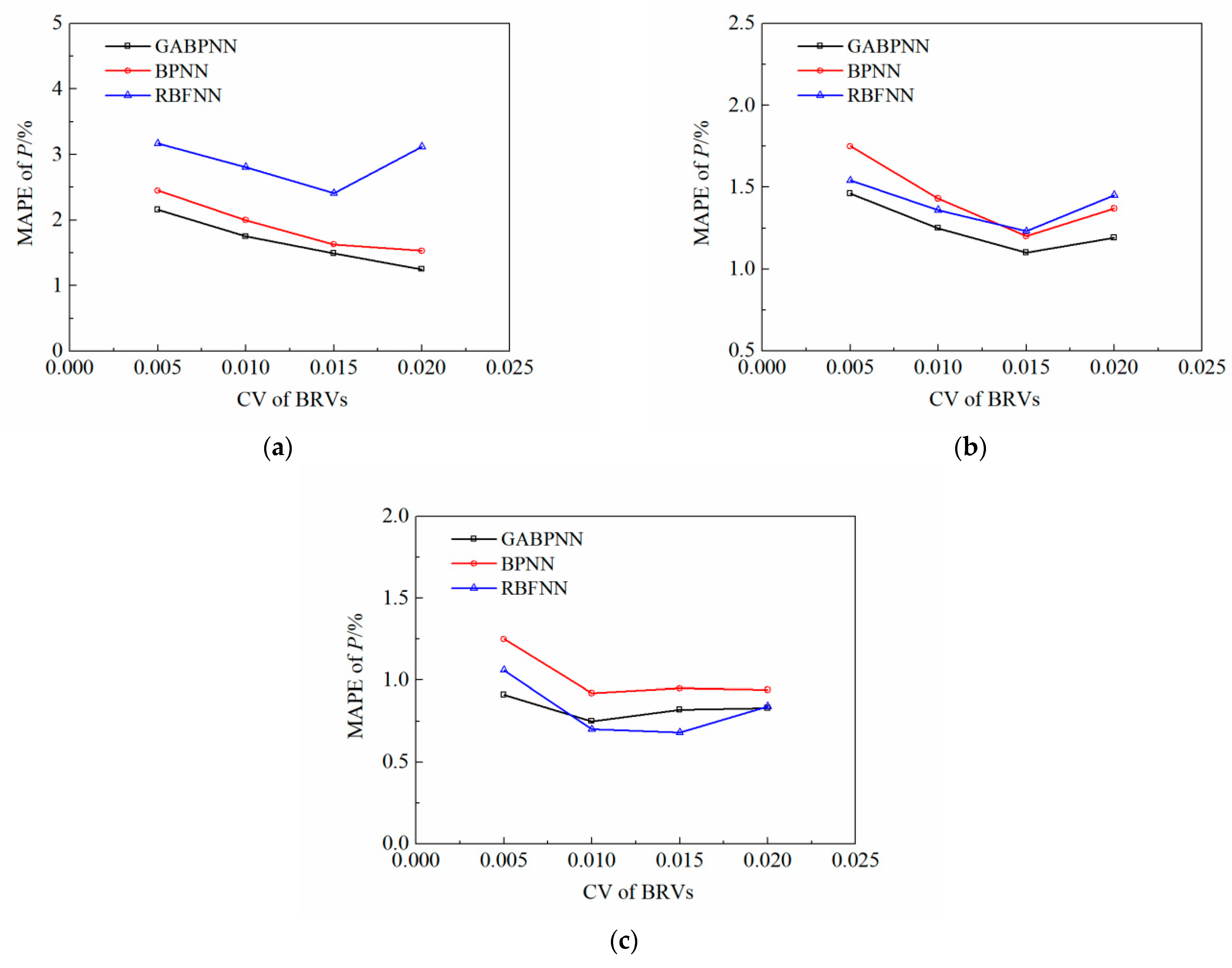
The test results in Table 7 and Figure 8 show that the GABPNN consistently had a Mean Absolute Percentage Errors (MAPE) lower than 2.2% in calculating the P of each gauge in the numerical model corresponding to these 4 test sample sets, and the MAPEs of the GABPNN were slightly higher than the corresponding ones of the RBFNN only when calculating the P of the gauge 3 corresponding to the test sample sets where the CVs of BRVs were respectively 0.01 and 0.015, and the MAPEs of the GABPNN were lower than the corresponding ones of the RBFNN and BPNN when calculating the P of each gauge under other conditions. It is proved that the GABPNN has stronger nonlinear mapping ability than the BPNN and RBFNN, and the GABPNN can accurately calculate the P of each gauge corresponding to the BRV sample points. Therefore, the GABPNN can be used as the surrogate model of the DPR, and the GABP-MCS can also be used to estimate the statistical characteristics of the P of each gauge of Composition B.

(iv) Estimation of the statistical characteristics of P based on GABP-MCS

The sample points that could lead Composition B to be initiated were selected from the prediction sample sets of the IP, so as to construct the prediction sample sets of the DPR. According to Table 6, in addressing the DPR, the 4 prediction sample sets, with the CVs of the BRVs being, respectively, 0.005, 0.01, 0.015, and 0.02, had 78,654, 66,291, 61,281, and 58,711 sample points, respectively. The calculation results of the P’s of the three gauges in the numerical model corresponding to these four prediction sample sets were obtained by the GABP-MCS, so as to obtain the accurate estimates of the actual statistical characteristics of the P’s of these three gauges under the above four randomness conditions, as shown in

Table 8. The calculation results of the GABP-MCS in the DPR study under the shock load condition where $\overline{v}$ is 1050 m/s.

Gauge Number		1				2				3
CV of BRVs		0.005	0.01	0.015	0.02	0.005	0.01	0.015	0.02	0.005	0.01	0.015	0.02
Statistical characteristic of P	Mean of P (GPa)	26.55	27.30	27.91	28.30	29.18	29.58	29.96	30.30	31.61	31.88	32.22	32.54
	CV of P	0.0618	0.0736	0.0824	0.0965	0.0271	0.0423	0.0567	0.0736	0.0228	0.0364	0.0509	0.0664

and Figure 9.

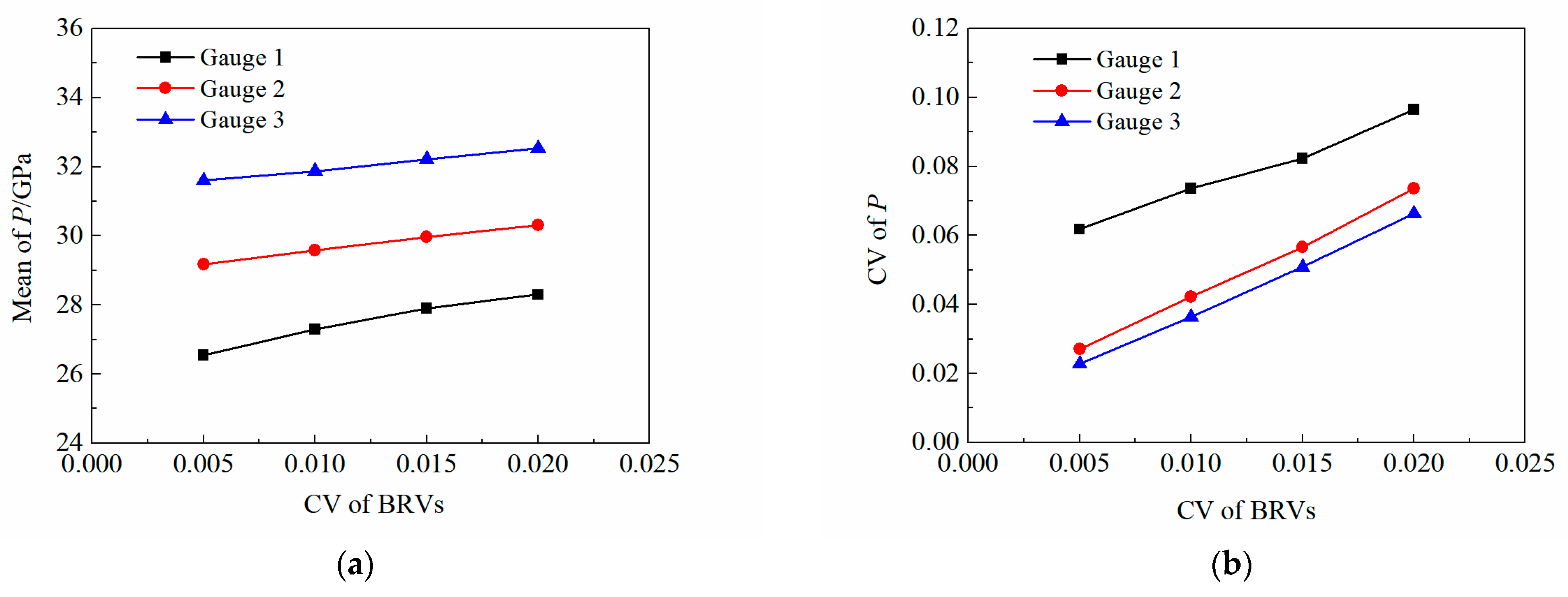
The following are the three observations from Table 8 and Figure 9 and their interpretation. First, for each gauge, the mean of its P is positively correlated with the CV of the BRVs; that is, the mean of its P can increase gradually with the CV of the BRVs. This is because the more likely the BRV sample points result in the initiation of Composition B, the greater P Composition B tends to generate in subsequent detonations. Furthermore, the larger the CV of the BRVs, the more scattered the distribution of the BRV sample points in the corresponding prediction sample sets, and the more BRV sample points that can result in lower values of the P will be eliminated in addressing the DPR for the initiation failure of Composition B. In this case, a higher proportion of the BRV sample points, which result in the higher values of the P in the prediction sample sets, suggests the higher estimated means of the P. What is also observed is that, under these four randomness conditions, the CVs of the P’s of the three gauges in the numerical model are all significantly larger than the CVs of the BRVs, which indicates that the randomness of the BRVs can magnify the randomness of the P. The third observation is that, for each gauge, the CV of its P is also positively correlated with the CV of the BRVs; that is, the CV of its P can decrease with the CV of the BRVs. This is because the smaller the CV of the BRVs, the lower the randomness of the SIREM and the lower the randomness of the P, which suggests the smaller the CV of the P. So, it can be further deduced that, if the CV of the BRVs dropped to 0, the SIREM would become a deterministic problem, the CVs of the P would also drop to 0, and the P would also become a deterministic variable accordingly.

4.3.2. Shock Load Condition Where $\overline{v}$ Is 1000 m/s

(1)

Study on IP

(i) Constructing training sample set and test sample sets

In addressing the IP when the $\overline{v}$ is 1000 m/s, in order to guarantee the excellent generalization ability of the ANNs and sufficient training sample points for the DPR, 3000 sample points were generated for the BRVs with the CV of 0.02, and 1000 sample points were generated for the BRVs with the CV of 0.005, so as to construct the training sample set with 4000 sample points. Then, a test sample set with 1000 sample points was constructed for the BRVs with each of the CVs of 0.005, 0.01, 0.015, and 0.02.

Table 9. The statistical results of the initiation and non-initiation frequencies of Composition B in the training sample set and test sample sets under the shock load condition where $\overline{v}$ is 1000 m/s.

Sample Set		Sample Size q	Initiation Frequency	Non-Initiation Frequency
Training sample set		4000	1580	2420
Test sample set	CV of BRVs being 0.005	1000	258	742
	CV of BRVs being 0.01	1000	367	633
	CV of BRVs being 0.015	1000	398	602
	CV of BRVs being 0.02	1000	454	546

shows the statistical results of the initiation and non-initiation frequencies of Composition B in these training sample set and test sample sets.

(ii) Determining the structure and important parameters of ANNs

In this stage, under the shock load condition that the $\overline{v}$ is 1000 m/s, the setting of the structure and important parameters of the GABPNN, BPNN, and RBFNN is the same as the corresponding operation under the shock load condition where the $\overline{v}$ is 1050 m/s; see Section 4.3.1.

(iii) Performance comparison of ANNs

Firstly, the GABPNN, BPNN, and RBFNN were trained by the above training sample set. Then, these three trained ANNs were tested by each of the above four test sample sets, and the test results shown in

Table 10. The comparison of the test results of the ANNs in the IP study under the shock load condition where $\overline{v}$ is 1000 m/s.

Test Sample Set		ANN Being Tested	δT Being the Same as δE		δT Being Different from δE		Accuracy of Testing (%)
CV of BRVs	Test Number		Both δT and δE Being 1	Both δT and δE Being 0	δT Being 1 and δE Being 0	δT Being 0 and δE Being 1
0.005	1000	GABPNN	196	684	58	62	88.0
		BPNN	198	667	75	60	86.5
		RBFNN	115	688	54	143	80.3
0.01	1000	GABPNN	311	572	61	56	88.3
		BPNN	309	567	66	58	87.6
		RBFNN	275	596	37	92	87.1
0.015	1000	GABPNN	341	553	49	57	89.4
		BPNN	334	542	60	64	87.6
		RBFNN	321	561	41	77	88.2
0.02	1000	GABPNN	405	504	42	49	90.9
		BPNN	390	503	43	64	89.3
		RBFNN	398	520	26	56	91.8

and Figure 10 were obtained.

According to the test results shown in Table 10 and Figure 10, the test accuracy when the GABPNN calculated the 0–1 recognition results of the δ corresponding to these 4 test sample sets was consistently higher than 87%, and the testing accuracy of the GABPNN was slightly lower than the corresponding one of the RBFNN only when calculating the 0–1 recognition results of the δ corresponding to the test sample set with the CV of BRVs as 0.02, and the testing accuracies of the GABPNN were higher than the corresponding ones of the RBFNN and BPNN when calculating the 0–1 recognition results of the δ under other conditions. It is proved that the GABPNN has stronger nonlinear mapping ability than the BPNN and RBFNN, and the GABPNN can accurately calculate the 0–1 recognition results of the δ corresponding to the BRV sample points. Therefore, the GABPNN can be used as the surrogate model of the IP, and the GABP-MCS can also be used to estimate the R’s of Composition B.

(iv) Estimation of R based on GABP-MCS

A prediction sample set with 100,000 sample points was constructed under each of the above 4 randomness conditions, and the 0–1 recognition results of the δ corresponding to these 4 prediction sample sets were obtained by the GABP-MCS, so as to obtain the accurate estimates of the actual R’s of Composition B under these 4 randomness conditions.

Table 11. The calculation results of the GABP-MCS in the IP study under the shock load condition where $\overline{v}$ is 1000 m/s.

CV of BRVs	Simulation Number	Initiation Frequency	Non-Initiation Frequency	R (%)
0.005	100,000	26,151	73,849	26.15
0.01	100,000	36,677	63,323	36.68
0.015	100,000	40,812	59,188	40.81
0.02	100,000	43,155	56,845	43.16

and Figure 11 show the results.

According to the statistical data in Table 11 and the correlation curve in Figure 11, it can be concluded that, when the $\overline{v}$ is 1000 m/s, the R of Composition B is positively correlated with the CV of the BRVs; that is, the smaller the CV of the BRVs, the lower the R of Composition B. This is because the smaller the CV of the BRVs, the more concentrated the distribution of the BRV sample points in the corresponding prediction sample sets, the less BRV sample points there are that can lead Composition B to be initiated, and the lower the randomness of the SIREM. If the CV of the BRVs dropped to 0, this SIREM would become a deterministic problem, so Composition B would not be initiated (the R would drop to 0) under the shock load condition where $\overline{v}$ was 1000 m/s, which would be exactly the same as the deterministic results described in Section 4.1.

(2)

Study on DPR

(i) Constructing training sample set and test sample sets

The same method discussed in Section 4.3.1 was adopted to construct the training sample set and test sample sets of the DPR. Table 9 shows that in addressing the DPR, the training sample set had 1580 sample points and the 4 test sample sets with 258, 367, 398, and 454 sample points, which correspond, respectively, to the CVs of the BRVs at 0.005, 0.01, 0.015, and 0.02.

(ii) Determining the structure and important parameters of ANNs

When the $\overline{v}$ is 1000 m/s, the setting of the structure and important parameters of the GABPNN, BPNN, and RBFNN is the same as the corresponding operation when the $\overline{v}$ is 1050 m/s; see Section 4.3.1 for the setting process.

(iii) Performance comparison of ANNs

Firstly, the GABPNN, BPNN, and RBFNN were trained by the above training sample set. Then, these three trained ANNs were tested by each of the above four test sample sets, and the test results shown in

Table 12. The comparison of the test results of the ANNs in the DPR study under the shock load condition where $\overline{v}$ is 1000 m/s.

Gauge Number		1				2				3
CV of BRVs		0.005	0.01	0.015	0.02	0.005	0.01	0.015	0.02	0.005	0.01	0.015	0.02
MAPE of P (%)	GABPNN	2.48	1.86	1.66	1.72	2.51	1.86	1.92	2.38	2.46	1.11	1.23	1.28
	BPNN	3.25	2.22	1.86	1.76	3.89	2.47	2.26	2.48	2.62	1.23	1.29	1.42
	RBFNN	3.06	3.16	2.87	3.34	4.03	2.90	2.83	3.68	2.74	1.54	1.61	2.04

and Figure 12 were obtained.

According to the test results shown in Table 12 and Figure 12, the GABPNN consistently had MAPEs lower than 2.6% in calculating the P of each gauge in the numerical model corresponding to these 4 test sample sets, and these test results were also better than the test results of BPNN and RBFNN. It is proved that the GABPNN has stronger nonlinear mapping ability than the BPNN and RBFNN, and the GABPNN can accurately calculate the P of each gauge corresponding to the BRV sample points. Therefore, the GABPNN can be used as the surrogate model of the DPR, and the GABP-MCS can also be used to estimate the statistical characteristics of the P of each gauge of Composition B.

(iv) Estimation of the statistical characteristics of P based on GABP-MCS

The sample points that could lead Composition B to be initiated were selected from the prediction sample sets of the IP, so as to construct the prediction sample sets of the DPR. According to Table 11, in addressing the DPR, the 4 prediction sample sets, with the CVs of the BRVs being, respectively, 0.005, 0.01, 0.015, and 0.02, had 26,151, 36,677, 40,812, and 43,155 sample points, respectively. The calculation results of the P’s of the three gauges in the numerical model corresponding to these four prediction sample sets were obtained by the GABP-MCS, so as to obtain the accurate estimates of the actual statistical characteristics of the P’s of these three gauges under the above four randomness conditions, as shown in

Table 13. The calculation results of the GABP-MCS in the DPR study under the shock load condition where $\overline{v}$ is 1000 m/s.

Gauge Number		1				2				3
CV of BRVs		0.005	0.01	0.015	0.02	0.005	0.01	0.015	0.02	0.005	0.01	0.015	0.02
Statistical characteristic of P	Mean of P (GPa)	24.96	26.61	27.44	28.06	28.33	29.34	29.90	30.38	31.25	32.05	32.45	32.80
	CV of P	0.0613	0.0804	0.0900	0.0991	0.0441	0.0552	0.0676	0.0829	0.0317	0.0406	0.0533	0.0674

and Figure 13.

The following are the three observations from Table 13 and Figure 13 and their interpretation. First, for each gauge, the mean of its P is positively correlated with the CV of the BRVs; that is, the mean of its P can increase with the CV of the BRVs. This is because the more likely the BRV sample points result in the initiation of Composition B, the greater P Composition B tends to generate in subsequent detonations. Furthermore, the larger the CV of the BRVs, the more scattered the distribution of the BRV sample points in the corresponding prediction sample sets, and the more BRV sample points that can result in higher values of the P will be reserved in addressing the DPR, for they can lead to the initiation of Composition B. This suggests the higher estimates of the means of the P. What is also observed is that, under these four randomness conditions, the CVs of the P’s of the three gauges in the numerical model are all significantly larger than the CVs of the BRVs, which indicates that the randomness of the BRVs can magnify the randomness of the P. The third observation is that, for any gauge, the CV of its P is also positively correlated with the CV of the BRVs; that is, the CV of its P can increase with the CV of the BRVs. This is because the larger the CV of the BRVs, the higher the randomness of the SIREM, and the higher the randomness of the P, which suggests the larger the CV of the P.

The above are the details of this applied example. The study results show that the shock response of Composition B has obvious randomness under the action of the main BRVs, and that the GABP-MCS can be adopted to solve the SIREM to obtain satisfactory randomness study results. Moreover, since Composition B is representative among various kinds of energetic materials, this example can also prove the universality of GABP-MCS in the study on SIREM.

5. Discussion

(1)

Selection of study methods of SIREM on a macroscopic scale

With many well-established stochastic analysis methods and the uniqueness of SIREM on a macroscopic scale, it is necessary to discuss the selection of the study methods of SIREM.

The common stochastic analysis methods available may fall into three broad types. The first type is semi-analytical methods, including such typical methods as the center point method [44,45], checking point method [46,47], and perturbation method [48,49]. In applying this type of method between BRVs and RRs, they must form a definite performance function, which must be continuously differentiable to BRVs so as to obtain the statistical analysis results of RRs through the derivative of the performance function to BRVs. The next type is MCS and its improved versions. This type, on the basis of the law of large numbers, conducts repeated sampling tests by selecting a large number of BRV sample points to obtain the corresponding statistical analysis results of RRs. The last type refers to surrogate model methods, represented by the response surface method [50,51], Kriging method [52,53,54], and artificial neural network (ANN) method. The philosophy of this type is that a substitute surrogate model for original calculation ones is constructed, together with the first two types of method, to obtain the statistical analysis results of RRs.

In the studies on SIREM on a macroscopic scale, semi-analytical methods may not apply, for it is nearly impossible to construct a definite performance function due to the quite complex nonlinear mapping between BRVs and RRs. It is impractical to adopt MCS or its improved versions, which directly use the numerical simulations of the shock initiation of energetic materials as repeated sampling tests, because the great amount of time required by these numerical simulations renders this type of method quite time- and effort-consuming. In addition, common surrogate model methods, such as the response surface method and Kriging method, may not fit the SIREM study either. This is because the marked differences in the RR values between the initiation and non-initiation states of energetic materials suggest the impossibility of forming an approximate continuous limit state surface between BRVs and RRs. Therefore, what can be adopted are the methods of combining the ANNs, which are more powerful in nonlinear mapping and quick enough in calculating, with MCSs in the SIREM study.

As GABPNN is an ANN with strong nonlinear mapping ability and high computational efficiency, the GABP-MCS with GABPNN as the surrogate model is adopted to solve SIREM in this paper. Yet, what should be noticed is that with the rapid development of machine learning and artificial intelligence, new ANNs with greater nonlinear mapping ability have been developed one after another, so it is necessary to try to apply other new ANNs to solve SIREM in future work.

(2)

Correlation between mesoscopic and macroscopic studies on SIREM

Although the mesoscopic studies on SIREM recorded in the literature [7,8,9,10,11,12,13,14,15,16,17,18,19,20,21] are limited to preliminary theoretical exploration under standard test conditions to obtain the initiation probabilities and probabilistic initiation thresholds of energetic materials, the effect of the indeterminacy of the microstructure of energetic materials on the impact sensitivity of energetic materials has been investigated. This can better explore the source of the impact sensitivity randomness of energetic materials; that is, the random distribution of the micro-sized energetic grains, binder grains, voids, and cracks inside the energetic materials is among the root causes of the impact sensitivity randomness of energetic materials, which may further the perceptions of the nature of this issue. On the other hand, although the macroscopic study on SIREM in this paper can obtain the initiation probabilities of energetic materials under more complex working conditions and the statistical characteristics of the detonation pressure in different positions inside these energetic materials after they are initiated, so as to better meet the needs of engineering practices, the source of the impact sensitivity randomness of energetic materials cannot be directly addressed by taking the parameters of the Lee–Tarver equation of reaction rate and the JWL equation of state as the BRVs of the detonation characteristics. This forms the limitations of solving SIREM on a macroscopic scale. In fact, our research team believes that the randomness of these parameters is the macroscopic manifestation of the randomness of the microstructure of energetic materials. Hence, these two kinds of randomness are equivalent and can both represent the randomness of the detonation characteristics of energetic materials, with the former being the macroscopic phenomenological representation of the randomness of the detonation characteristics of energetic materials, and the latter being the mesoscale source.

Therefore, due to the complementary relationship between the mesoscopic and macroscopic SIREM studies, it is suggested that researchers should conduct studies from both perspectives to make the fullest use of them. In addition, no well-established theoretical methods are now available to conduct a quantitative study of the effects of the microstructure randomness of energetic materials on the parameter randomness of the Lee–Tarver equation of reaction rate and the JWL equation of state. This indicates the absence of a unified research system that involves the detonation characteristic randomness of energetic materials, as well as its phenomenological representation and natural representation, which requires further study in the future.

6. Conclusions

The macroscopic SIREM study should explore in turn the R’s of energetic materials and the randomness of P after energetic materials are initiated, so it is natural to decompose SIREM into IP and DPR. The main BRVs on the detonation characteristics of energetic materials can be selected from the parameters a, I, b, x, G₁, c, d, y, G₂, e, g, and z in the Lee–Tarver equation of reaction rate and the parameters A_c, B_c, R_c1, R_c2, w_c, A_g, B_g, R_g1, R_g2, and w_g in the JWL equation of state. The main BRVs on shock load conditions can be selected from the physical quantities, such as the mass m, shock velocity v, and shock angle θ of a fragment. In IP, δ should be introduced as RR. In DPR, the P of energetic materials should be defined as RR.

The macroscopic SIREM study should adopt the method of combining ANN surrogate models with MCSs due to the quite complex nonlinear mapping between RRs and BRVs. Therefore, this paper uses GABPNNs as the surrogate models of the numerical models of two-phase reactive flow, adopts GABP-MCS to solve SIREM, and develops the approaches.

To verify the effectiveness of GABP-MCS in solving SIREM and to provide the specific solving processes, the shock initiation randomness problem of Composition B is taken as an applied example in this paper. Under the randomness conditions that the $\overline{v}$’s are 1050 m/s and 1000 m/s and that the CVs of the BRVs are 0.005, 0.01, 0.015, and 0.02, the R’s of Composition B and the statistical characteristics, such as the means and CVs of the P of Composition B, are obtained, and the variation tendencies that these statistics show under various randomness conditions are further observed.

In a nutshell, this paper analyzes SIREM on a macroscopic scale and proposes the approach of adopting GABP-MCS to solve SIREM, so as to develop a universal technique for calculating the initiation probabilities of energetic materials under complex working conditions and the statistical characteristics of detonation pressure. This technique can be widely applied to engineering practices, such as assessments of the shock safety randomness of energetic materials.

In addition, as mentioned in Discussion 5, GABPNN is just a mature ANN, and it is necessary to try to apply other new ANNs to solve SIREM in future work. Moreover, no well-established theoretical methods are now available to conduct a quantitative study of the effects of the microstructure randomness of energetic materials on the parameter randomness of the Lee–Tarver equation of reaction rate and the JWL equation of state, which requires further study in the future.