Three-Dimensional Modeling of Heart Soft Tissue Motion

Abstract

The modeling and simulation of biological tissue is the core part of a virtual surgery system. In this study, the geometric and physical methods related to soft tissue modeling were investigated. Regarding geometric modeling, the problem of repeated inverse calculations of control points in the Bezier method was solved via re-parameterization, which improved the calculation speed. The base surface superposition method based on prior information was proposed to make the deformation model not only have the advantages of the Bezier method but also have the ability to fit local irregular deformation surfaces. Regarding physical modeling, the fitting ability of the particle spring model to the anisotropy of soft tissue was improved by optimizing the topological structure of the particle spring model. Then, the particle spring model had a more extensive nonlinear fitting ability through the dynamic elastic coefficient parameter. Finally, the secondary modeling of the elastic coefficient based on the virtual body spring enabled the model to fit the creep and relaxation characteristics of biological tissue according to the elongation of the virtual body spring.

1. Introduction

Traditional medical surgery carries out preoperative simulation and determines the operation plan based on historical data and experience, but the process is seriously affected by subjective factors. With the appearance of virtual surgery simulation, a more objective preoperative simulation becomes possible. As the specific application of virtual reality technology in the medical field, virtual surgery simulation is gradually becoming the research object of scientific researchers in various countries [1].

In the research of biological tissue modeling, modeling can be simply divided into two categories according to whether force calculation is included, namely, physical modeling and geometric modeling [2]. Geometric modeling is mainly used to describe and express the shape of an object. In the modeling process, the influence of force is not considered, and the accuracy of the shape is emphasized. Meanwhile, physical modeling is based on physical principles, and the process of model change is determined through internal force calculations. Therefore, the structure is more complex.

The earliest geometric modeling was realized as a wireframe, which only described the shape of the object through basic points, lines, and surfaces. This method could not be applied to more complex situations [3]. In 1963, Ferguson [4] of the United States introduced a cubic Hermite interpolation curve and expressed the curve and surface with a parameter vector function. Since then, the parametric form has become the main form of curve and surface shape descriptions.

The most classical method used in geometric modeling is the Bezier method [5] proposed by Pierre Bezier, a French engineer. He defined curves and surfaces by controlling polygons and converted complex surface control into relatively simple polygon control. This method greatly reduces the complexity of modeling and has good overall shape control ability.

In the following years, the Bezier method was continuously improved by adjusting the basis function of the Bezier method. Deboor and Cox gave the standard algorithm of a B-spline based on the Bezier method [6]. Later, Riesenfel and Versprille respectively studied a non-uniform B-spline [7] and a rational B-spline [8]. The B-spline method can solve the problem of insufficient local control in the Bezier method, and the surface order is independent of the number of vertices. However, the B-spline method has a big problem that it cannot describe the surface in a unified curve and surface expression form [9].

In the early 1990s, Piegl and Tiller proposed a non-uniform rational B-spline (NURBS) method based on rational B-spline [10]. This method can represent many surfaces by adjusting the weight factors and node vectors. Although it has the problem of high complexity and improper parameter selection that may lead to distortion, it has become the most widely used geometric modeling method because it has a common mathematical form for arbitrary curves and surfaces and has good local control ability.

Geometric modeling methods include the chain mail model [11], but the curve and surface model based on the Bezier method has always been the mainstream of geometric modeling. The pure Bezier method is mostly used in industrial design, and its modeling accuracy is improved in terms of two aspects: one is to improve the order of the Bezier method [12] and the other is to optimize the basis function [13,14], such as the NURBS method. In the field of soft tissue modeling, simple geometric modeling is no longer competent, and physical modeling is added on this basis. Current mainstream physical modeling methods include the finite element method and particle spring model [15], which have their advantages and disadvantages and should be selected according to the relevant characteristics of soft tissue [16].

The finite element method and particle spring model are often used for the physical modeling of biological tissue [17]. According to the characteristics of the two, many biological tissue modeling researchers have proposed different optimization ideas and methods.

For the finite element model, R. J. Lapeer et al. proposed a human skin hyperelastic finite element model for interactive real-time surgical simulation [18], which effectively improved the simulation effect of the finite element model on the elastic model; M. Freute et al. discussed the relevant characteristics and internal forces of various soft tissues, provided relevant theoretical support for soft tissue modeling, and carried out a simple implementation of the finite element method [19]; Plantefève finally realized simple liver simulation by reducing the computational complexity based on finite element analysis [20]. H. Talbot realized the overall model construction of the heart by using finite elements, improved the program efficiency through multi-threaded calculation, and realized simple intracardiac navigation [21]. It can be seen that based on the finite element method, the improvement direction is mostly to improve the calculation efficiency. On the other hand, due to the complicated process of the finite element method, it is difficult to expand its simulation capability [22].

For the mass–spring model, W. Mollemans et al. realized the tetrahedral mass–spring model, giving the mass–spring model a better sense of volume [23]; Y. Duan et al. [24] introduced a new position constraint into the mass–spring model to fit the incompressibility of soft tissue and make it more consistent with the actual characteristics; A. Okamura [25] reduced the superelastic phenomenon of the model by optimizing the dynamic equation of the spring and prevented the excessive distortion of the deformation process under special circumstances; W. Mollemans et al. [23] put forward the concept of a virtual body spring based on the particle spring model. By introducing the original state of the model into the model change process, the elastic deformation process of the soft tissue model is more real, and the design of the three-dimensional mass–spring model proposed by Vicente, G.S. et al., which expands the dimension of the mass–spring model [26]. In terms of the particle spring model, the focus of improvement is its more characteristic description ability, and the adaptability of the particle spring model in the field of soft tissue modeling is improved by introducing more parameters [15].

Although there were many breakthroughs in the common methods of physical modeling, the physical modeling method itself is more complex than geometric modeling, how to establish a physical model with accurate results and high calculation efficiency is still an urgent problem to be solved [27].

In this study, first, the geometric modeling of heart soft tissue motion modeling and visualization was investigated. Based on the research of common geometric modeling methods, the Bezier method was used to conduct soft tissue geometric modeling. Combined with the shortcomings of the Bezier method in the field of soft tissue modeling, optimization was carried out. Second, the physical modeling of heart soft tissue motion modeling and visualization was studied. Through the research and analysis of common physical modeling methods, this study used the particle spring model to realize the physical modeling of the heart’s soft tissue surface and combined the biological characteristics of biological tissue to optimize the classical particle spring model. Finally, the relevant optimization process was verified via a simulation.

2. Materials and Methods

2.1. Re-Parameterization of Bezier Surface Modeling

The Bezier method has a very fast calculation speed in the case of a few control points and can ensure that the surface is smooth in the case of any control point arrangement. It is generated by interpolating the control points based on the Bernstein basis function, given as Equations (2) and (3). At the same time, the model established using the Bezier method is completely and only determined by the relative positions of the control points. Therefore, this method can ensure the same modeling with the control point data and facilitate surface reconstruction. Therefore, the Bezier method is the basis of many commonly used methods [28,29]. This study gave full play to the advantages of the classical Bezier method, and at the same time, puts forward some improved ideas and methods for its shortcomings.

If $m\times n$ control points $P_{ij}$ are given in a known space, let

$$p_{m-1,n-1}(u,v)={\displaystyle \sum _{i=0}^{m-1}{\displaystyle \sum _{j=0}^{n-1}{B}_{i,m-1}(u)B_{j,n-1}(v)}}{P}_{ij}$$

(1)

where $i=0,1,\dots ,m-1$, $j=0,1,\dots ,n-1$, the surface $p_{m,n}(u,v)$ represented by Formula (1) is a Bezier surface determined by $m\times n$ control points, and $B_{i,m}(u)$ and $B_{j,n}(v)$ are Bernstein basis functions of different orders:

$$B_{i,m}(u)=C_m^i{u}^i{(1-u)}^{m-i}=\frac{m!}{i!(m-i)!}{u}^i{(1-u)}^{m-i}$$

(2)

$$B_{j,n}(v)=C_n^j{v}^j{(1-v)}^{n-j}=\frac{n!}{j!(n-j)!}{v}^j{(1-v)}^{n-j}$$

(3)

where $u\in [0,1],v\in [0,1]$.

The data used in the geometric modeling process in this study was the actual collected cardiac local surface position information, and each frame was composed of a $3\times 3$ dot matrix. According to the definition of a Bezier surface, it is known that the surface is a biquadratic Bezier surface, and its expression is

$$\begin{array}{ll}{p}_{2,2}(u,v)& ={\displaystyle \sum _{i=0}^2{\displaystyle \sum _{j=0}^2{B}_{i,2}(u)B_{j,2}(v)}}{P}_{ij}\\ & ={(1-u)}^2{(1-v)}^2{P}_{00}+2{(1-u)}^{2}v(1-v)P_{01}+{(1-u)}^2{v}^2{P}_{02}\\ & +2u(1-u){(1-v)}^2{P}_{10}+4u(1-u)v(1-v)P_{11}+2u(1-u)v^2{P}_{12}\\ & +u^2{(1-v)}^2{P}_{20}+2u^{2}v(1-v)P_{21}+2u_2{v}^2{P}_{22}\end{array}$$

(4)

The matrix form is

$$p_{2,2}(u,v)=\left[\begin{array}{ccc}{u}^2& u& 1\end{array}\right]\left[\begin{array}{ccc}1& -2& 1\\ -2& 2& 0\\ 1& 0& 0\end{array}\right]\left[\begin{array}{ccc}{P}_{00}& P_{01}& P_{02}\\ P_{10}& P_{11}& P_{12}\\ P_{20}& P_{21}& P_{22}\end{array}\right]\left[\begin{array}{ccc}1& -2& 1\\ -2& 2& 0\\ 1& 0& 0\end{array}\right]\left[\begin{array}{c}{v}^2\\ v\\ 1\end{array}\right]$$

(5)

where $p_{2,2}(u,v)$ represents the coordinates of any point on the surface and $B_{i,2}(u)$ and $B_{j,2}(v)$ are second-order Bernstein basis functions, where the control point coordinates are

$$\left[\begin{array}{ccc}{P}_{00}& P_{01}& P_{02}\\ P_{10}& P_{11}& P_{12}\\ P_{20}& P_{21}& P_{22}\end{array}\right]$$

The Bezier surface geometric modeling process needs to know the control point coordinates, and the Bezier surface calculates the points on the surface through the control points and parameters $u,v$. Therefore, to calculate the coordinates of the control points, we need to know not only the points on the surface but also the parameters $u,v$. Since the data set approximately represents a uniform rectangular area, the $u,v$ corresponding to each coordinate point in this case is

$$\left[\begin{array}{ccc}(1,0)& (1,0.5)& (1,1)\\ (0.5,0)& (0.5,0.5)& (0.5,1)\\ (0,0)& (0,0.5)& (0,1)\end{array}\right]$$

The control point coordinates corresponding to the surface can be inversely calculated according to Formula (4), and then the biquadratic Bezier surface can be determined according to the Bezier surface given in Formula (1).

Considering that the Bezier surface definition requires known control points but the data set acquisition usually obtains mismatching of surface points, this study re-parameterized Equation (4) so that the coordinates of the data set can be directly brought into the formula for Bezier surface modeling and calculation, thus saving a lot of the control point coordinate calculation process. Through experimental calculation, under the same conditions, the model’s FPS (frames per second) without an improved calculation process is about 250 FPS and the improved FPS is about 280 FPS, which improves the system efficiency.

The specific re-parameterization method is as follows.

For the biquadratic Bezier surface with a $3\times 3$ dot matrix, set the data points collected in advance and the control points of the corresponding Bezier surface as follows:

$$\left[\begin{array}{ccc}{P}_{20}^0& P_{21}^0& P_{22}^0\\ P_{10}^0& P_{11}^0& P_{12}^0\\ P_{00}^0& P_{01}^0& P_{02}^0\end{array}\right],\left[\begin{array}{ccc}{P}_{20}& P_{21}& P_{22}\\ P_{10}& P_{11}& P_{12}\\ P_{00}& P_{01}& P_{02}\end{array}\right]$$

Since the coordinates of the data points are approximately evenly distributed at equal intervals, the distribution is as shown in the figure.

Then, we can know from the endpoint position property of the Bezier surface that

$$\left\{\begin{array}{c}{P}_{00}=P_{00}^0\\ P_{02}=P_{02}^0\\ P_{20}=P_{20}^0\\ P_{22}=P_{22}^0\end{array}\right.$$

(6)

Then, according to Figure 1 and Equation (4), the expression of the remaining data points is calculated as follows:

$$\left\{\begin{array}{l}{P}_{01}^0=p_{2,2}(0,\frac{1}{2})=\frac{1}{4}{P}_{00}+\frac{1}{2}{P}_{01}+\frac{1}{4}{P}_{02}\hfill \\ P_{10}^0=p_{2,2}(\frac{1}{2},0)=\frac{1}{4}{P}_{00}+\frac{1}{2}{P}_{10}+\frac{1}{4}{P}_{20}\hfill \\ P_{11}^0=p_{2,2}(\frac{1}{2},\frac{1}{2})=\frac{1}{16}{P}_{00}+\frac{1}{8}{P}_{01}+\frac{1}{16}{P}_{02}+\frac{1}{8}{P}_{10}+\frac{1}{4}{P}_{11}+\frac{1}{8}{P}_{12}+\frac{1}{16}{P}_{20}+\frac{1}{8}{P}_{21}+\frac{1}{16}{P}_{22}\hfill \\ P_{12}^0=p_{2,2}(\frac{1}{2},1)=\frac{1}{4}{P}_{02}+\frac{1}{2}{P}_{12}+\frac{1}{4}{P}_{22}\hfill \\ P_{21}^0=p_{2,2}(1,\frac{1}{2})=\frac{1}{4}{P}_{20}+\frac{1}{2}{P}_{21}+\frac{1}{4}{P}_{22}\hfill \end{array}\right.$$

(7)

Combining Equations (6) and (7), the solution is

$$\left\{\begin{array}{l}{P}_{00}=P_{00}^0\hfill \\ P_{01}=-\frac{1}{2}{P}_{00}^0+2P_{01}^0-\frac{1}{2}{P}_{02}^0\hfill \\ P_{02}=P_{02}^0\hfill \\ P_{10}=-\frac{1}{2}{P}_{00}^0+2P_{10}^0-\frac{1}{2}{P}_{20}^0\hfill \\ P_{11}=\frac{1}{4}{P}_{00}^0-P_{01}^0+\frac{1}{4}{P}_{02}^0-P_{10}^0+4P_{11}^0-P_{12}^0+\frac{1}{4}{P}_{20}^0-P_{21}^0+\frac{1}{4}{P}_{22}^0\hfill \\ P_{12}=-\frac{1}{2}{P}_{02}^0+2P_{12}^0-\frac{1}{2}{P}_{22}^0\hfill \\ P_{20}=P_{20}^0\hfill \\ P_{21}=-\frac{1}{2}{P}_{20}^0+2P_{21}^0-\frac{1}{2}{P}_{22}^0\hfill \\ P_{22}=P_{22}^0\hfill \end{array}\right.$$

(8)

If Formula (8) is substituted into Formula (4), the following can be obtained:

$$\begin{array}{ll}{p}_{2,2}(u,v)& =(1-u)(1-2u)(1-v)(1-2v)P_{00}^0+4(1-u)(1-2u)v(1-v)P_{01}^0\\ & -(1-u)(1-2u)v(1-2v)P_{02}^0+4u(1-u)(1-v)(1-2v)P_{10}^0\\ & +16u(1-u)v(1-v)P_{11}^0-4u(1-u)v(1-2v)P_{12}^0\\ & -u(1-2u)(1-v)(1-2v)P_{20}^0-4u(1-2u)v(1-v)P_{21}^0\\ & +u(1-2u)v(1-2v)P_{22}^0\end{array}$$

(9)

The re-parameterization result of the biquadratic Bezier surface under the distribution of control points is shown in Formula (9). When used, the measurement data can be substituted into the above formula, eliminating the step of calculating control points.

For any Bezier surface modeling, although the results of re-parameterization are affected by the number of control points and the distribution of control points, the distribution of the measured data points can usually be determined in the process of manual measurement, and the measurement area is relatively fixed. Therefore, the re-parameterization method has certain universality. The ideas are summarized as follows.

If it is known that the modeling calculation formula of any Bezier surface is Formula (1), then the following process can take place:

Step 1: According to the endpoint position property of the Bezier surface, the control points at the four vertices of the surface are $p_{m,n}(0,0)$, $p_{m,n}(0,1)$, $p_{m,n}(1,0)$, and $p_{m,n}(1,1)$, and their values are equal to the four vertices at the corresponding positions of the measurement data set.

Step 2: According to the overall distribution of the data points in the measurement data set, the parameters corresponding to each point can be determined, that is, the $p_{m,n}(u,v)$ corresponding to each data point can be determined. Then, according to the Bezier surface Formula (1), the equations represent each data point with control points, i.e., $m\times n$ equations, including the four equations obtained in step 1.

Step 3: Solve the $m\times n$ equations and rewrite them into the form of expressing control points with data points. There must not be two identical equations in the $m\times n$ equations, and thus, it can only find one expression, that is, the correspondence between the finally determined data points and control points.

Step 4: Replace the control points in Formula (1) according to the corresponding relationship between the data points and the control points, that is, obtain the surface calculation formula after re-parameterization.

The above method solves the problem that the control points in the Bezier method are not on the surface to some extent via re-parameterization. The data obtained in the actual measurement process are generally of the same distribution, and thus, only one reverse calculation process is required, which greatly improves the dynamic modeling efficiency of the Bezier method.

2.2. Base Surface Superposition Based on Prior Information

Since the control points in the Bezier method control the shape of the surface as a whole, the change in the control points will inevitably cause a change in the surface as a whole, making the model as smooth as possible in any case. However, this characteristic also causes the Bezier method to be unable to accurately fit many local characteristics of the object, such as the edges and corners in the local area.

To achieve this goal and enable the Bezier method to retain the inherent characteristics of the fitting object to a certain extent, this study proposed a method of superimposing the base surface according to prior information and the Bezier method. This method can introduce the local irregular characteristics of the object through the base surface while maintaining the smooth and continuous characteristics of the Bezier surface.

The stacking process can be roughly divided into two parts.

First, the local measurement of the object is used to fit a surface used to describe the inherent local irregular characteristics of the object, which is called the base surface. The surface needs to retain the surface details of the object, and thus, there are certain requirements for the accuracy of prior information.

After that, the base surface is superimposed and the calculation formulas of the two are fused. In the subsequent process, the data used by the base surface will not change, and thus, the Bezier surface will not be affected in the dynamic state.

After introducing the inherent characteristics of the base surface, the local characteristics will not affect the overall smoothness, and the invariance of the inherent characteristics can be guaranteed in the process of change. The superimposed base surface can easily introduce local characteristics. When the model accuracy is low, it will degenerate into a separate Bezier surface and still be able to complete the modeling work.

2.3. Anisotropic Optimization of the Particle Spring Model

In the classical particle spring model, the bending spring makes the influence range of a single particle larger by connecting the spaced particles. It is precisely because of the increase in this influence range that the edge of the deformation region is smooth [15]. However, due to the structure of the bending spring, this ability is relatively more concentrated in the vertical and horizontal directions. Compared with uniform elastic physics, because it does not have anisotropy, the demand for the control ability in different directions is not high. However, for special objects, such as soft tissue surfaces, anisotropy as an important characteristic requires stronger control ability. Inspired by a bending spring, a spring can be added in the diagonal direction so that the model can more accurately represent the anisotropy in more directions.

After introducing this kind of diagonal spring, the topological structure of the particle spring model becomes as shown in Figure 2. This topological structure retains the three types of springs in the classical particle spring model and adds a new type of spring. For the convenience of description, this paper refers to it as a reinforcing spring, which connects two particles separated by a particle in a diagonal direction. The main purpose is to give the particle stronger control ability in the diagonal direction. Through the combination of a reinforcing spring and a complete spring, the particle can cope with changes in more directions to fit more complex soft tissue heterogeneity.

To verify that the bending spring and the reinforcing spring have different control capabilities for the motion of the particle in different directions, this paper explains this through mathematical calculations. The process is as follows.

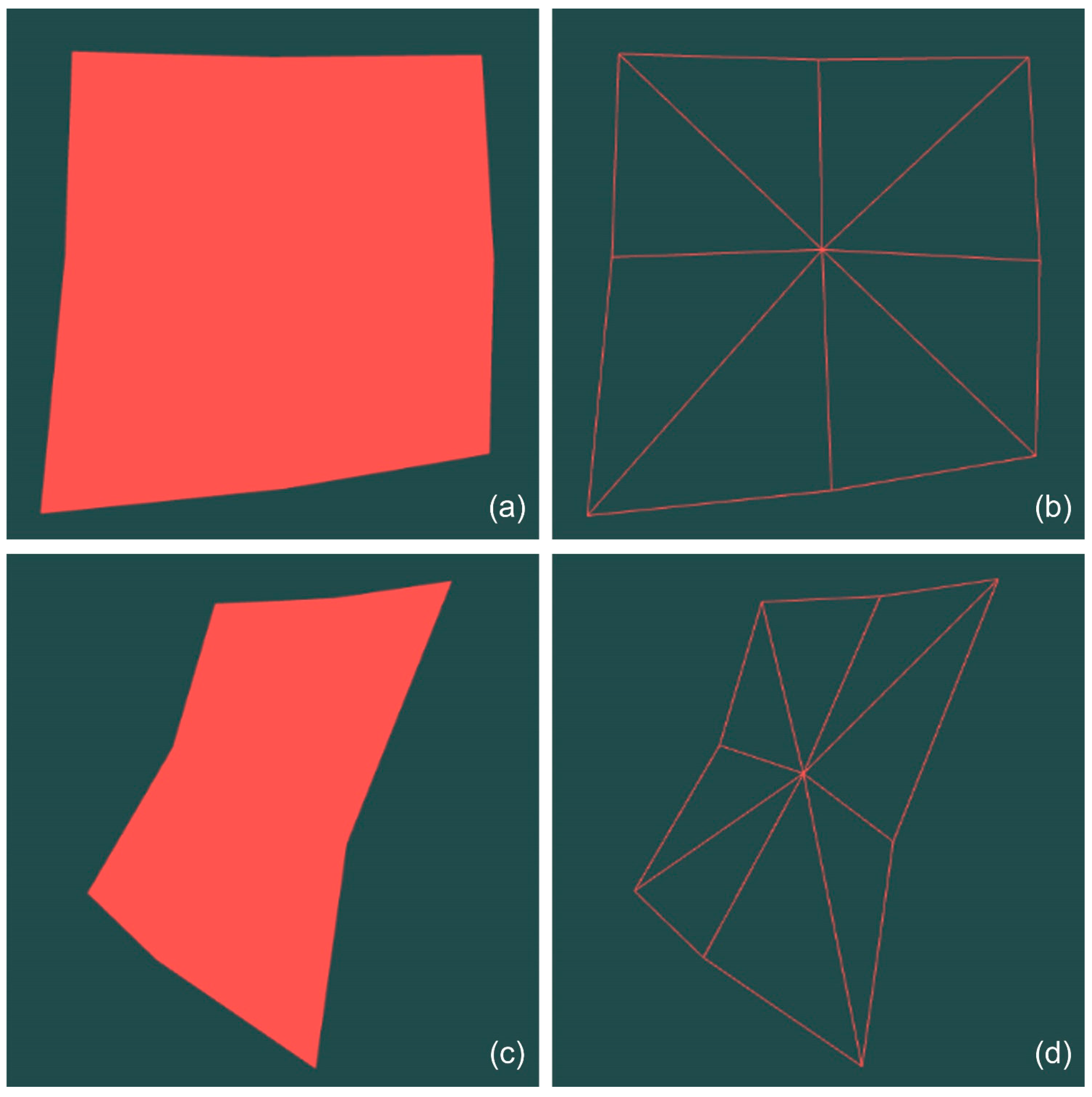
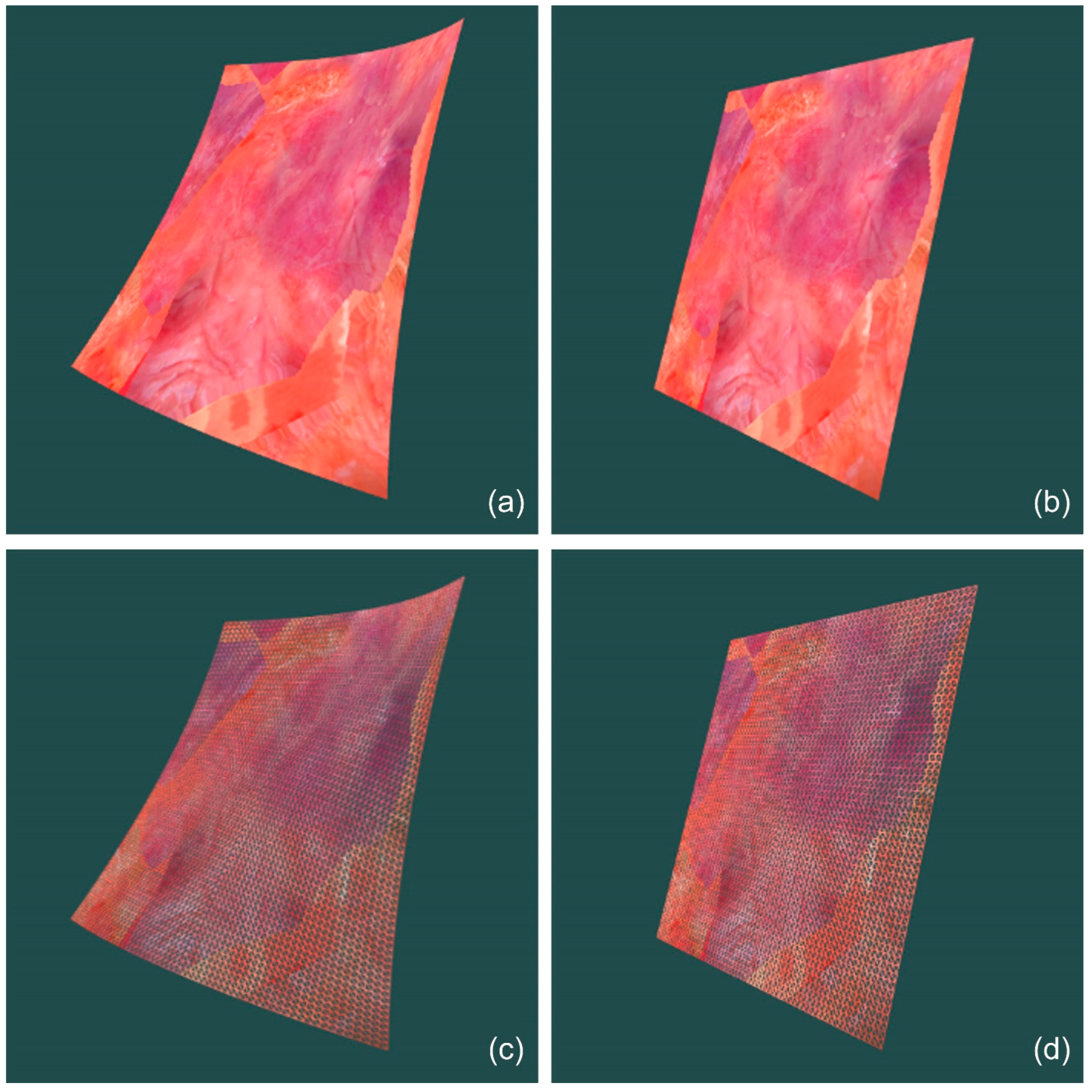
In the verification process, to minimize the interference of other factors, only two structures of the bending spring and reinforcing spring are retained. In the object model, the particle is located at the intersection of the grid composed of squares with a side length of 1, and the elastic coefficient of all springs is 1. The relaxation length is the distance between the particles in the grid at the time of initialization, and the calculation process uses a unified measurement standard, omitting the unit. The specific position of the particle in the experimental model is shown in Figure 3a, and the bending spring and the reinforcing spring are shown in Figure 3b,c.

The verification process is divided into two parts:

• Move the particle at the center to the left by 0.5, as shown in Figure 4a,b.
• Move the particle at the center upward to the right, as shown in Figure 4c,d.

After that, the forces generated by different structures on the central particle in each of the two cases are calculated. The calculation results are shown in

Table 1. Comparison of the force of bending and reinforcing spring on particle change.

Spring Category	Lateral Movement 0.5		Move Upright $\frac{\sqrt{2}}{2}$
	Direction	Size	Direction	Size
Bending spring	Horizontal left	1.211	Lower left	1.040
Reinforcing spring	Horizontal left	1.110	Lower left	1.563

.

Through the calculation results of the two changes, it can be found that the control ability of the bending spring was stronger than that of the reinforcing spring in the transverse change process, and the control ability of the reinforcing spring in the diagonal direction was stronger than that of the bending spring, that is, the control ability of the two types of springs to the same change in the particle was different. Therefore, this showed that the method of improving the ability of the model to fit soft tissue heterogeneity by optimizing the topological structure of the particle spring model was effective.

2.4. Nonlinear Relationship Fitting Based on Parameter Dynamics

It is known that the dynamic equation of the basic unit in the mass–spring model can be expressed as

$$f_b=k(l-l^0)+cv$$

(10)

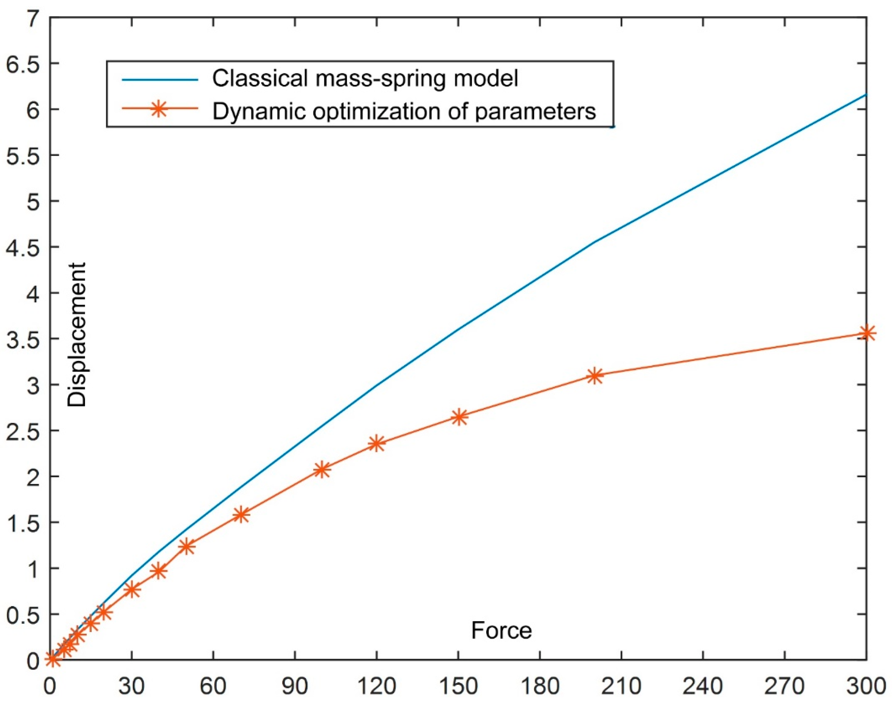
Among them, the elastic coefficient $k$ and the damping coefficient $c$ are constants representing the inherent characteristics of the spring and the damper, respectively. The particle spring model can fit the elastic deformation under normal conditions due to its internal structure composed of springs. However, because its dynamic equation is relatively simple, it cannot fit the nonlinear relationship between the stress and strain of biological tissues well [2]. In order to improve the ability of the mass–spring model in this respect, this study proposed to dynamically change the original constant elastic coefficient with the change in the corresponding spring length, thereby introducing a continuous nonlinear mapping to enable it to fit the more complex stress–strain relationship. This method is called parameter dynamics.

The ultimate purpose of this improvement is to control the changing relationship between the force and displacement of the particle through the dynamic elastic coefficient to fit the nonlinear relationship between the force and deformation of the biological tissue. During the modeling process, the force and deformation of the soft tissue correspond to the external force and displacement of the particle, respectively. Therefore, first, we need to find the relationship between the elastic coefficient $k$ and the force and displacement of the particle. In the mass–spring model, the process of deformation can be roughly expressed as follows: the mass is accelerated by the external force, and thus, the displacement occurs such that the length of the connecting spring of the mass changes and the elastic force is generated to balance the impact of the external force on the mass. In this process, the damping force is generated at the same time, and the hysteresis phenomenon occurs. After that, the force between the particles continues to spread. Finally, when the resultant force of all the particles is zero, the model reaches a new equilibrium state.

Theoretically, since the non-mapping relationship between the elastic coefficient and the corresponding spring length change is arbitrary, the fitting can also be arbitrary. However, considering the computational cost required by this method, the nonlinear relationship with a lower order should be selected as much as possible. Here, to show that the dynamic elasticity of this parameter can indeed introduce a nonlinear relationship, the derivation formula is as follows:

$$\begin{array}{ll}F& =f_e+{\displaystyle \sum _{n=1}^{n=m}[k^n(l^n-l^{n0})+c^{n}v]}\\ & =f_e+{\displaystyle \sum _{n=1}^{n=m}(l^n-l^{n0})}{\displaystyle \sum _{n=1}^{n=m}{k}^n}+{\displaystyle \sum _{n=1}^{n=m}{c}^{n}v}\end{array}$$

(11)

If the mapping relationship between the elastic coefficient $k^n$ of any spring and the corresponding spring length change $(l^n-l^{n0})$ is shown in Equation (12), where $h^n$ represents the constant coefficient of the linear mapping

$$k^n=h^n(l^n-l^{n0})$$

(12)

Then, according to Formula (11):

$$F=f_e+{\displaystyle \sum _{n=1}^{n=m}{(l^n-l^{n0})}^2}{\displaystyle \sum _{n=1}^{n=m}{h}^n}+{\displaystyle \sum _{n=1}^{n=m}{c}^{n}v}$$

(13)

The above formula shows that there is a nonlinear relationship between the external force on the particle and the change in the spring length after the parameter is dynamic.

$$s=\frac{1}{2}a{t}^2=\frac{1}{2}\frac{F}{m}{t}^2=\frac{1}{2}\frac{t^2}{m}{f}_e+\frac{1}{2}\frac{t^2}{m}{(l-l^0)}^{2}h+\frac{1}{2}\frac{t^2}{m}cv$$

(14)

The above formula shows that the displacement of the particle and the change in the spring length also have a nonlinear relationship, and thus, it can be concluded that the nonlinear mapping of the basic element of any model can make the external force of the particle and the displacement of the particle have a nonlinear relationship.

To sum up, compared with the classical particle spring model, this study introduced the mapping of Formula (12) to achieve a more accurate nonlinear relationship between the force and displacement of particles, which showed that the method of introducing the nonlinear relationship through parameter dynamics was effective, and because this mapping relationship was not unique, the fitting nonlinear relationship had great flexibility. At the same time, in the same model, the nonlinear relations in different regions and directions could be realized by different mappings of different springs.

2.5. Viscoelastic Control Based on a Virtual Body Spring

Considering that the spring mesh in the mass–spring model is only distributed on the surface of the model, the control ability of the mass–spring model to the model object is mostly concentrated on the surface of the model, which leads to the inflexibility of the mass–spring model in fitting the changes in the direction perpendicular to the surface. The reason for this is that the mass–spring model itself does not have variables that describe the characteristics in the vertical direction, this problem was significantly improved with the appearance of virtual body springs [26].

The method using virtual body springs is relatively simple, that is, the real-time position of the particle in the particle spring model and the corresponding initial position are connected by a virtual spring, and the relaxation length of the virtual spring is 0. The reason why it is called a virtual body spring is that the spring does not exist before the model changes, and it will only work after the model changes.

During the process of model deformation, the force generated by the virtual body spring is dynamic. After the model loses the external force, all the particles can reach the stable state when they are at the initial position, that is, the model can finally recover to the initial state through the force generated by the virtual body spring.

The main purpose of the virtual body spring method proposed by the original author is to give the model a sense of volume [26], and the model can automatically return to the original state after removing the external force, which can make the simulation of elastic deformation of the particle spring model more realistic. However, the virtual body spring enables the particle spring model to obtain the control ability in the vertical surface direction. Based on this, this study undertook further research and, inspired by the dynamic parameters mentioned above, some improvements were made to the virtual body spring to enhance the ability of the model to fit the biological characteristics in the vertical surface direction.

The two previous optimizations are mainly used to improve the particle spring in response to the characteristics of soft tissue anisotropy and stress–strain nonlinearity. However, the spring mesh is coincident with the curved surface, and thus, it is difficult to show the viscoelasticity of biological tissue in the vertical direction, including creep, relaxation, and hysteresis [16]. To solve this problem, a method was proposed in this study. Based on the virtual body spring structure, the elastic coefficient in the virtual body spring is remapped to make the elastic force produced by the virtual body spring more consistent with the viscoelastic characteristics.

The virtual body spring is still special in essence and the elastic force generated by it can be expressed as

$$f_v=Kl+cv$$

(15)

In this study, the remapping of the elastic coefficient K was used to make Formula (15) better fit the viscoelasticity of biological tissue. Since the function of the damper itself is to reflect the hysteresis characteristics of elastic objects in the deformation process, to reduce the complexity of remapping, this study aimed to use the damper to fit the hysteresis characteristics and fit the creep and relaxation characteristics of biological tissue through remapping. To fit the above characteristics, first, it was necessary to determine the relationship between the force and the creep relaxation reaction.

Generally, the creep characteristic is mainly manifested in the process of biological tissue deformation, while the relaxation characteristic is mainly manifested in the process of biological tissue restitution [19]. In terms of creep characteristics, when biological tissue is deformed from the initial state, even if the initial force is relatively small, the tissue will appear obviously offset, but the effect of the force on the offset distance will rapidly decrease with the increase in the offset distance of the object. For relaxation characteristics, because it is mainly manifested in the recovery process, the initial recovery state should be subject to a large force and the recovery speed is faster. As the offset distance between the object and the initial state becomes smaller and smaller, the recovery speed will become slower and slower. To understand this relationship more clearly, this study established an approximate relationship between the force and the object’s offset distance using the creep and relaxation characteristics in general.

Since the virtual body spring connects the actual position of the mass point and the corresponding initial position, and the relaxation length is 0, which makes the spring elongation equal to the displacement of the mass point, the change in the mass point can be judged using the change in the elongation of the virtual body spring corresponding to the mass point, that is, the model is in the process of stress deformation when the virtual body spring is extended, and the model is in the process of restoring the initial state when the virtual body spring is shortened.

From this, it can be seen that the creep characteristic shown in Figure 5a can be fitted when the virtual body spring is extended, and the relaxation characteristic shown in Figure 5b can be fitted when the spring is shortened. It is obvious that the approximate change relationship is nonlinear, but it can be seen from Equation (15) that the existing virtual body spring cannot realize the nonlinear relationship between the spring extension amount and the generated force. In the previous article, the parameter dynamic method was proposed to give the spring the ability to fit the non-linear relationship, which led us to consider the following: if the elastic coefficient of the virtual body spring is remapped, can it better fit the viscoelasticity of biological tissue?

The remapping process of the spring elastic coefficient of the virtual body is represented by Equation (16):

$$k=f(l)$$

(16)

Then:

$$f_v=f(l)l+cv$$

(17)

It can be seen from Figure 5a,b that the changing relationship corresponding to the two characteristics is different, but both can be approximated as a quadratic curve. To fit the relationship, Equation (16) is expressed as:

$$k=h_{1}l+h_2+h_3\frac{1}{l}$$

(18)

where $h_1$, $h_2$, and $h_3$ are adjustable parameters. If Equation (18) is substituted into Equation (17), we obtain

$$f_v=h_1{l}^2+h_{2}l+h_3+cv$$

(19)

Through the above derivation, it can be shown that the creep and relaxation characteristics obtained by any measurement can be approximated using this mapping method, but different mapping relationships need to be selected when describing the creep and relaxation characteristics of the same model.

2.6. Calculation Process for the Physical Modeling

The calculation process for the particle spring model is roughly divided into two steps. The first step is to solve the acceleration of the particle, and the second step is to solve the position of the particle at the next time according to the acceleration obtained by the particle.

In the improved mass–spring model, the force acting on a single mass can be expressed as

$$F=f_{st}+f_{sh}+f_{\mathrm{be}}+f_{\mathrm{en}}+f_{\mathrm{vi}}+f_e$$

(20)

where $f_{st}$ is the elastic force generated by the structural spring, $f_{sh}$ is the elastic force generated by the shear spring, $f_{be}$ is the elastic force generated by the bending spring, $f_{en}$ is the elastic force generated by the reinforcing spring, $f_{vi}$ is the elastic force generated by the virtual body spring, and $f_e$ is the external force applied at this point. The force $f$ generated by any basic unit in the model can be expressed as

$$f=f(l-l^0)(l-l^0)+cv$$

(21)

where $f(l-l^0)$ represents the mapping of the spring elastic coefficient, $l$ represents the spring length at the current time, $l^0$ represents the spring relaxation variable, $c$ represents the damping coefficient, and $v$ represents the current velocity of the particle.

The sum of the external forces on a single particle can be calculated using Equations (20) and (21), and then the acceleration $a$ of the particle can be obtained according to $F=ma$. Thus, the first step of the calculation process is completed. The acceleration $a$ is mainly determined by the parameters in the mass–spring model. The results of this process are controlled by adjusting the parameters and then entering the parameters to the second step of the calculation process.

The second step involves solving the position of the particle after the change. It is assumed that the initial position of the particle is $s_0$, the initial velocity is $v_0$, the initial acceleration is $a_0$, and the time step is t. Among the above parameters, $a_0$ can be obtained in step 1, $s_0$ is the data obtained via an advance measurement, and the time step is an adjustable parameter. Combined with $v=at$ and $s=\frac{1}{2}a{t}^2$, the following can be obtained:

$$v_t=v_0+a_{0}t$$

(22)

$$s_t=s_0+v_{0}t+\frac{1}{2}{a}_0{t}^2$$

(23)

where $v_t$ represents the velocity of the particle at the next time and $s_t$ represents the position of the particle at the next time. This completes the second step of the calculation process. The result generated in this step is determined by the acceleration generated in step 1 and cannot be controlled. The model can be updated by the position of the particle at the next time obtained in this step.

When fitting the force deformation of the model, the total force of the particle changes. The acceleration is calculated in step 1, and then the new position is calculated in step 2 to determine whether the resultant force of the particle at the new position is zero. If the force on all the particles is zero under the current situation, the model will reach a new equilibrium state. If there are particles with a non-zero force, repeat the calculation process of step 1 and step 2 so that the position of the particles will continue to be updated. From a macro perspective, this shows the force deformation process of the model. When the resultant force on all the particles is zero, the particles will not generate new acceleration and displacement. At this time, the model is in a stable state.

3. Results

3.1. Effect and Explanation of the Geometric Modeling of Heart Soft Tissue

3.1.1. Implementation of the Single Frame Model

Static model data: select the data of nine coordinate points in the first frame of the measurement data set and use the Bezier method to conduct biquadratic Bezier surface modeling. The model surface color is set to red. The modeling effect is shown in Figure 6.

In this case, since no interpolation operation was carried out, this model only included nine coordinate data points of the measurement data. Because the number of points was too small, there were fewer triangular patches, and there were obvious boundaries at the intersection of triangular patches. Based on the above two points, the model was far from usable. Next, the optimization and improvement of the model are discussed.

3.1.2. Model Effect Optimization

To make the model smooth, it is necessary to increase the number of nodes to increase the number of triangular patches. Because the measurement data are limited, the interpolation method was used to increase the number of nodes to improve the accuracy of the model. At the same time, considering the observation problem, texture mapping was introduced to greatly improve the observation effect. The result was shown in Figure 7.

As can be seen from Figure 7, the surface was very smooth after thinning. At the same time, due to the existence of texture, it was easier to observe. The refined model met the modeling requirements in terms of accuracy, and the degree of thinning could be freely controlled.

3.1.3. Dynamic Effect Display

The model could finally achieve 800 frames of continuous dynamic display. Here, the model changes between different times are explained by comparing the models at different times. To see the consistency of the model changes and the difference, two discontinuous models were selected for result verification, as shown in Figure 8.

3.1.4. Re-Parameterization Validity Verification

In this study, the calculation speed of the modeling process was improved using re-parameterization. To show that the re-parameterization method will not lead to a shape change in the model, the two methods of re-modeling through reverse calculation of control points and directly modeling with the re-parameterized calculation formula were compared to show the correctness of the method. The first frame data were still selected for the experiment.

It can be seen from Figure 9 that the reparameterization did not change the shape of the model, and then the fps line chart for ten consecutive moments in the two cases was plotted, as shown in Figure 10, it can be seen that the reparameterization under the same conditions improves the fps of the program, thus proving the effectiveness of the reparameterization method.

3.1.5. Base Surface Overlay Verification

Since there is no other relevant data on the object area in the research process, to verify the effectiveness and feasibility of the superimposed base surface method, we chose to manually extract part of the object features to build the base surface. In the extraction process, first, the plane close to the surface was determined as the reference, and the plane coordinate data were compared with the original surface coordinate data. The new data retained the details of each position of the surface, and the data were superimposed on the base surface.

In theory, the model will become a plane after the base surface is superimposed. To verify the effectiveness of the base surface superimposition, a simulation experiment was conducted here.

Compared with the original surface, as shown in Figure 11a,c, combined with the experimental results of the superimposed base surface Figure 11b,d, it can be found that the superimposed base surface does introduce new information into the original surface, and does not modify the data related to the original surface in this process, which shows that it is feasible to make the model retain the inherent properties of the object through the base surface.

3.2. Effect and Explanation of the Physical Modeling of Heart Soft Tissue

3.2.1. Force Verification of the Optimized Mass–Spring Model

In this study, the classical particle spring model was first realized in the research process, and then its adaptability to soft tissue fitting was improved through optimization. Here, the correctness of the optimized particle spring model was verified by calculating the force of each particle in the initial state and the external force.

In the initial state of the particle spring model, the position and force of the particle are shown in

Table 2. Initial position and stress of particle.

Particle Data	Particle Coordinate Position	Force on Particle
First point	2.449, −5.161, 43.124	0.000, 0.000, 0.000
Second point	5.597, −5.083, 42.853	0.000, 0.000, 0.000
Third point	8.698, −5.136, 42.088	0.000, 0.000, 0.000
Fourth point	2.508, −2.281, 41.294	0.000, 0.000, 0.000
Fifth point	5.550, −2.241, 41.133	0.000, 0.000, 0.000
Sixth point	8.599, −2.287, 41.717	0.000, 0.000, 0.000
Seventh point	2.612, 0.480, 40.384	0.000, 0.000, 0.000
Eighth point	5.550, 0.444, 39.870	0.000, 0.000, 0.000
Ninth point	8.581, 0.434, 40.607	0.000, 0.000, 0.000

.

It can be seen from Table 2 that each mass point was at the actual measurement position, and since the relaxation length of each spring was equal to the distance between the mass points connected to the spring, no elastic force was generated. The above data were in line with the expected situation.

After that, we applied a stable force (0, 10, 20) to the central particle, that is, the fifth particle, and observed the position and force of the particle.

At the moment of force on the particle, the force on the fifth particle was unbalanced, and the model started to change. The instantaneous force on the particle is shown in

Table 3. Instantaneous position and force of the particle.

Particle Data	Particle Coordinate Position	Force on Particle
First point	2.449, −5.161, 43.124	0.000, 0.000, 0.000
Second point	5.597, −5.083, 42.853	0.000, 0.000, 0.000
Third point	8.698, −5.136, 42.088	0.000, 0.000, 0.000
Fourth point	2.508, −2.281, 41.294	0.000, 0.000, 0.000
Fifth point	5.550, −2.241, 41.133	0.000, 10.000, 20.000
Sixth point	8.599, −2.287, 41.717	0.000, 0.000, 0.000
Seventh point	2.612, 0.480, 40.384	0.000, 0.000, 0.000
Eighth point	5.550, 0.444, 39.870	0.000, 0.000, 0.000
Ninth point	8.581, 0.434, 40.607	0.000, 0.000, 0.000

.

After that, all particles continued to change and finally returned to the equilibrium state, and

Table 4. Position and force of particles in the model under a balanced stress state.

Particle Data	Particle Coordinate Position	Force on Particle
First point	2.449, −5.161, 43.124	0.000, 0.000, 0.000
Second point	5.606, −5.099, 42.863	−0.003, 0.012, −0.004
Third point	8.698, −5.136, 42.088	0.000, 0.000, 0.000
Fourth point	2.534, −2.285, 41.306	0.000, 0.003, −0.002
Fifth point	5.560, −1.966, 41.764	−0.005, 0.002, 0.002
Sixth point	8.628, −2.295, 41.721	−0.008, 0.004, −0.001
Seventh point	2.612, 0.480, 40.384	0.000, 0.000, 0.000
Eighth point	5.557, 0.416, 39.900	0.002, 0.002, −0.003
Ninth point	8.581, 0.434, 40.607	0.000, 0.000, 0.000

was obtained.

It can be seen from Table 4 that the force of the fifth particle basically returned to zero, that is, the model returned to the stable state again. At this time, the position of each particle changed compared with the initial state. In particular, the force of the fifth point changed greatly, that is, the model realized the stress deformation process.

After that, the applied stabilizing force was removed, and the final model successfully returned to a stable state. The actual data output is shown in

Table 5. Position and stress of particles after the recovery.

Particle Data	Particle Coordinate Position	Force on Particle
First point	2.449, −5.161, 43.124	0.000, 0.000, 0.000
Second point	5.598, −5.077, 42.857	0.000, −0.001, 0.000
Third point	8.698, −5.136, 42.088	0.000, 0.000, 0.000
Fourth point	2.509, −2.274, 41.307	0.001, 0.000, 0.000
Fifth point	5.549, −2.270, 41.068	0.000, 0.001, 0.000
Sixth point	8.596, −2.286, 41.719	0.000, 0.000, 0.000
Seventh point	2.612, 0.480, 40.384	0.000, 0.000, 0.000
Eighth point	5.550, 0.442, 39.884	0.000, −0.001, 0.000
Ninth point	8.581, 0.434, 40.607	0.000, 0.000, 0.000

.

Therefore, the particles returned to their initial positions and completed the whole process of stress deformation.

3.2.2. Topology Optimization Effect Verification

In this study, a reinforcing spring was added based on the topological structure of the classical particle spring model. To verify that the introduction of the reinforcing spring improved the model’s ability to fit the anisotropy, the two cases where the elastic coefficients of the reinforcing spring and the bending spring were adjusted were compared in this experiment.

Since the original measurement data was a lattice, it was impossible to add a reinforcing spring. To experiment, this study first constructed a uniform lattice, then established a bicubic Bezier surface, introduced an optimized particle spring model, and created a model object. The experimental steps are as follows:

• The elastic coefficient of the bending spring was set to 2.0 and the elastic coefficient of the reinforcing spring was set to 10.0, a continuous force (0, 75, 0) was applied to the sixth mass point of the model, and the positions of each mass point were recorded when the model reaches the equilibrium state.
• The set value of the elastic coefficient of the bending spring and the reinforcing spring was adjusted, the same force was applied at the same position again, and the position of the mass was recorded again after the model was balanced.

The initial position of each particle and the measurement results under two conditions are shown in

Table 6. Initial positions of the particles and the effect of springs.

Particle Data	The Initial Position of a Particle	Large Bending Spring Coefficient	The Reinforced Spring Coefficient Is Large
First point	−3.000, 0.000, 45.000	−3.000, 0.000, 45.000	−3.000, 0.000, 45.000
Second point	−1.000, 0.000, 45.000	−0.998, 0.192, 44.994	−1.002, 0.184, 44.981
Third point	1.000, 0.000, 45.000	0.996, 0.105, 44.998	0.996, 0.104, 44.998
Fourth point	3.000, 0.000, 45.000	3.000, 0.000, 45.000	3.000, 0.000, 45.000
Fifth point	−3.000, 0.000, 43.000	−2.994, 0.192, 42.998	−2.981, 0.184, 43.002
Sixth point	−1.000, 0.000, 43.000	−0.989, 0.568, 42.989	−0.980, 0.649, 42.980
Seventh point	1.000, 0.000, 43.000	0.999, 0.150, 42.999	0.999, 0.144, 42.997
Eighth point	3.000, 0.000, 43.000	2.987, 0.076, 43.001	2.993, 0.034, 43.004
Ninth point	−3.000, 0.000, 41.000	−2.998, 0.105, 41.004	−2.997, 0.104, 41.004
Tenth point	−1.000, 0.000, 41.000	−0.999, 0.150, 41.001	−0.997, 0.144, 41.001
Eleventh point	1.000, 0.000, 41.000	0.999, 0.073, 41.001	0.998, 0.070, 41.002
Twelfth point	3.000, 0.000, 41.000	2.999, 0.001, 41.000	3.004, 0.001, 40.997
Thirteenth point	−3.000, 0.000, 39.000	−3.000, 0.000, 39.000	−3.000, 0.000, 39.000
Fourteenth point	−1.000, 0.000, 39.000	−1.001, 0.076, 39.013	−1.004, 0.034, 39.007
Fifteenth point	1.000, 0.000, 39.000	1.000, 0.001, 39.001	1.003, 0.001, 38.996
Sixteenth point	3.000, 0.000, 39.000	3.000, 0.000, 39.000	3.000, 0.000, 39.000

.

3.2.3. Nonlinear Effect Verification of the Parameter Dynamics

To verify that the model with dynamic parameters had a better nonlinear fitting ability, different forces were applied to a single particle in the classical particle spring model, the displacement data of the particle were recorded, and the relationship between the force and the displacement was found.

After that, the parameter dynamics was introduced, the elastic coefficient in the mass–spring model was mapped into Equation (12), and the mass displacement was recorded under the same force. The following Figure 12 was obtained.

3.2.4. Display of the Stress Deformation Effect

The previous experiments verified the correctness of the theory by calculating the force of each particle in the particle spring model. The purpose of this experiment was to show the change effect of the model after physical modeling under the external force from a macro perspective.

After applying a stable (0, 10, 20) force to the model in the initial state, the equilibrium state could be reached eventually. To facilitate observation of the change effect, a mesh with a low subdivision density was selected. The experimental results are shown in Figure 13.

4. Discussion

It can be seen from Figure 9 that the re-parameterization did not change the shape of the model, and then the FPS broken line diagram of ten consecutive times in both cases was drawn. As shown in Figure 10, it can be seen that the re-parameterization improved the FPS of the program under the same conditions, thus showing the effectiveness of the re-parameterization method.

Compared with the original surface, as shown in Figure 11, combined with the experimental results of the superimposed base surface, it was found that the superimposed base surface indeed introduced new information to the original surface, and the relevant data of the original surface was not modified in this process. Therefore, it is feasible for the model to retain the inherent characteristics of the object through the base surface.

In the experiment to verify the reinforced spring coefficient, the acting force position was the sixth mass point. Comparing the coordinate positions of the sixth mass point in the two cases, it was found that under the same situations, when the elastic coefficient of the reinforcing spring was large, the displacement of the mass point in the direction of the acting force was large. The reason for this was that the reinforcing spring only had a little restriction on the movement of the mass point perpendicular to the curved surface, and thus, the mass point could move farther under the same acting force. It was also found that, compared with the former case, when the coefficient of the reinforcing spring was large, the displacement of the same particle in the oblique direction was larger. Through the above two points, the reinforcing spring indeed had a stronger control ability in the diagonal direction of the particle than the bending spring.

It can be seen from Figure 11 that after the parameter dynamic mapping using Equation (12), the displacement of the particle was smaller than that before the optimization, and the larger the force, the larger the displacement deviation between the two, that is, the change amount of the particle displacement gradually decreased with the increase in the force. It was shown that the parameter dynamic method could indeed improve the nonlinear fitting ability of the mass–spring model to a certain extent, and the nonlinear mapping of the parameter dynamics could also be extended.

5. Conclusions

First, the classical geometric modeling method was studied, and the Bezier method was used to realize the geometric modeling of the heart’s soft tissue surface. After that, the modeling method was optimized to meet the requirements of ensuring real-time computations and improving authenticity. The huge waste caused by repeated calculation of control points was solved using the re-parameterization method, and the program running efficiency was improved. At the same time, considering the inherent characteristics of biological tissues, a base surface superposition method was proposed, which enabled the geometric model to retain details while maintaining the advantages of the Bezier method. The experimental results showed that the relevant optimization method for the Bezier method was effective, which not only improved the calculation speed but also makes it more widely applicable. At the same time, it can be seen from the model implementation effect that the model area under the Bezier method was very smooth.

Second, related research on physical modeling was carried out. Because ensuring real-time calculations is the highest priority in the virtual simulation process, the particle spring model was selected to realize the physical modeling of the heart’s soft tissue surface. However, the existing mass–spring model could not fully adapt to the problem of biological tissue modeling. Therefore, while representing the relevant characteristics of biological tissue, this study produced some optimization and improvement on the mass–spring model. First of all, through the optimization of the topological structure of the particle spring, its fitting ability to the anisotropy was improved. After that, the mass–spring model had a more extensive nonlinear relationship fitting ability through the dynamic parameter of the elastic coefficient. Finally, based on the virtual body spring, the second modeling of the elastic coefficient was carried out, and the creep and relaxation characteristics of biological tissue were fitted according to the change in the spring length. In the above three points, the mass–spring model was optimized for the anisotropy, nonlinearity, and viscoelasticity of biological tissue to improve its adaptability to the physical modeling of biological tissue. After the above theoretical research, relevant practical verification was also carried out. It can be seen from the realization effect of the model that the surface of the model was still smooth during the process of force change, and the deformation effect was consistent with the actual situation.

References

1. Li, H. Establishment of Emergency Teaching Model and Optimization of Discrete Dynamic Calculation in Complex Virtual Simulation Environment. Math. Probl. Eng. 2022, 2022, 6767237. [Google Scholar] [CrossRef]
2. Zou, Y.; Liu, P.X. A High-Resolution Model for Soft Tissue Deformation Based on Point Primitives. Comput. Methods Programs Biomed. 2017, 148, 113–121. [Google Scholar] [CrossRef] [PubMed]
3. Cotin, S.; Delingette, H.; Ayache, N. Real-Time Elastic Deformations of Soft Tissues for Surgery Simulation. IEEE Trans. Vis. Comput. Graph. 1999, 5, 62–73. [Google Scholar] [CrossRef] [Green Version]
4. Fuchs, L.; Bechmann, D.; Bertrand, Y.; Dufourd, J.F. Formal Specification for Free-Form Curves and Surfaces. In Proceedings of the Spring Conference on Computer Graphics, Bratislava, Slovakia, 5–7 June 1996. [Google Scholar]
5. Woźny, P.; Chudy, F. Linear-Time Geometric Algorithm for Evaluating Bézier Curves. Comput.-Aided Des. 2020, 118, 102760. [Google Scholar] [CrossRef]
6. Beccari, C.V.; Casciola, G. A Cox-De Boor-Type Recurrence Relation for C1 Multi-Degree Splines. Comput. Aided Geom. Des. 2019, 75, 101784. [Google Scholar] [CrossRef]
7. Deng, C.; Wang, Z.; Liu, J.; Xu, H.; Hu, Q. FC-NURBS Curves: Fullness Control Non-Uniform Rational B-Spline Curves. Commun. Inf. Syst. 2022, 22, 131–146. [Google Scholar] [CrossRef]
8. Hagen, H.; Bonneau, G.P. Variational Design of Smooth Rational Bézier Curves. Comput. Aided Geom. Des. 2018, 8, 393–399. [Google Scholar] [CrossRef] [Green Version]
9. Shi, F. Computer Aided Geometric Design and Non-Uniform Rational B-Spline; Higher Education Press: Beijing, China, 2001. [Google Scholar]
10. Zimmermann, C.; Sauer, R.A. Adaptive Local Surface Refinement Based on LR NURBS and Its Application to Contact. Comput. Mech. 2017, 60, 1011–1031. [Google Scholar] [CrossRef] [Green Version]
11. Gibson, S.; Fyock, C.; Grimson, E.; Kanade, T.; Kikinis, R.; Lauer, H.; McKenzie, N.; Mor, A.; Nakajima, S.; Ohkami, H.; et al. Volumetric Object Modeling for Surgical Simulation. Med. Image Anal. 1998, 2, 121. [Google Scholar] [CrossRef] [Green Version]
12. Han, X.A.; Ma, Y.C.; Huang, X.L. A Novel Generalization of Bézier Curve and Surface. J. Comput. Appl. Math. 2008, 217, 180–193. [Google Scholar] [CrossRef]
13. Hu, F.; Wu, J.; Qin, X. A Novel Extension of the Bézier Model and Its Applications to Surface Modeling. Adv. Eng. Softw. 2018, 125, 27–54. [Google Scholar] [CrossRef]
14. Li, J. A Class of Cubic Trigonometric Bezier Curve with a Shape Parameter. J. Inf. Comput. Sci. 2013, 10, 3071–3077. [Google Scholar] [CrossRef]
15. Andrew, N. Physically Based Deformable Models in Computer Graphics. Comput. Graph. Forum 2006, 25, 809–837. [Google Scholar]
16. Zhang, J.; Zhong, Y.; Gu, C. Deformable Models for Surgical Simulation: A Survey. IEEE Rev. Biomed. Eng. 2018, 11, 143–164. [Google Scholar] [CrossRef] [Green Version]
17. Cen, S.; Wu, C.J.; Li, Z.; Shang, Y.; Li, C. Some Advances in High-Performance Finite Element Methods. Eng. Comput. 2019, 36, 2811–2834. [Google Scholar] [CrossRef] [Green Version]
18. Lapeer, R.J.; Gasson, P.D.; Karri, V. A Hyperelastic Finite Element Model of Human Skin for Interactive Real-Time Surgical Simulation. IEEE Trans. Biomed. Eng. 2011, 58, 1013–1022. [Google Scholar] [CrossRef]
19. Freutel, M.; Schmidt, H.; Dürselen, L.; Ignatius, A.; Galbusera, F. Finite Element Modeling of Soft Tissues: Material Models, Tissue Iinteraction and Challenges. Clin. Biomech. 2014, 29, 363–372. [Google Scholar] [CrossRef]
20. Plantefève, R.; Peterlik, I.; Haouchine, N.; Cotin, S. Patient-Specific Biomechanical Modeling for Guidance during Minimally-Invasive Hepatic Surgery. Ann. Biomed. Eng. 2016, 44, 139–153. [Google Scholar] [CrossRef]
21. Talbot, H.; Spadoni, F.; Duriez, C.; Sermesant, M.; O’Neill, M.; Jaïs, P.; Cotin, S.; Delingette, D. Interactive Training System for Interventional Electrocardiology Procedures. Med. Image Anal. 2017, 35, 225–237. [Google Scholar] [CrossRef] [Green Version]
22. Taylor, Z.R.; Zhu, J. The Finite Element Method: Its Basis and Fundamentals; Butterworth–Heinemann: Oxford, UK, 2005. [Google Scholar]
23. Mollemans, W.; Schutyser, F.; Cleynenbreugel, J.V.; Suetens, P. Tetrahedral Mass Spring Model for Fast Soft Tissue Deformation. In Proceedings of the International Symposium on Surgery Simulation and Soft Tissue Modeling, Juan-Les-Pins, France, 12–13 June 2003; Springer: Berlin/Heidelberg, Germany, 2003; pp. 145–154. [Google Scholar]
24. Duan, Y.; Huang, W.; Chang, H.; Chen, W.; Zhou, J.; Teo, S.K.; Su, Y.; Chui, C.K.; Chang, S. Volume Preserved Mass-Spring Model with Novel Constraints for Soft Tissue Deformation. IEEE J. Biomed. Health Inform. 2015, 20, 268–280. [Google Scholar] [CrossRef]
25. Okamura, A.M.; Simone, C.; O’leary, M.D. Force Modeling for Needle Insertion into Soft Tissue. IEEE Trans. Biomed. Eng. 2004, 51, 1707–1716. [Google Scholar] [CrossRef] [PubMed]
26. Vicente, G.S.; Aguinaga, I.; Celigueta, J.T. Cubical Mass-Spring Model Design Based on a Tensile Deformation Test and Nonlinear Material Model. IEEE Trans. Vis. Comput. Graph. 2012, 18, 228–241. [Google Scholar] [CrossRef] [PubMed]
27. Schill, M. Biomechanical Soft Tissue Modeling Techniques, Implementation and Applications; Universitä Mannheim: Deutschland, Germany, 2001. [Google Scholar]
28. Nowak, M.; Michoński, J.; Sitnik, R. Filling Cavities in Point Clouds Representing Human Body Surface Using Bezier Patches. Multimed. Tools Appl. 2021, 80, 15093–15134. [Google Scholar] [CrossRef]
29. Joseph, L.; Tong, L.; John, M. Non-Linear Least Squares Fitting of Bezier Surfaces to Unstructured Point Clouds. AIMS Math. 2021, 6, 3142–3159. [Google Scholar]
Figure 1. Distribution of the data points.
Applsci 13 02493 g001
Figure 2. Schematic diagram of an anisotropic optimization topology.
Applsci 13 02493 g002
Figure 3. Schematic diagram of the experimental model: (a) schematic diagram of the particle distribution, (b) schematic diagram of the bending spring, and (c) schematic diagram of the reinforcing spring.
Applsci 13 02493 g003
Figure 4. Schematic diagram of the verification process: (a) schematic diagram of the lateral change in the bending spring, (b) schematic diagram of the lateral change in the reinforcing spring, (c) schematic diagram of the change in the bending spring at the upper right, and (d) schematic diagram of the change in the reinforcement spring at the top right.
Applsci 13 02493 g004
Figure 5. Graph of force versus object offset distance: (a) creep characteristics and (b) relaxation characteristics.
Applsci 13 02493 g005
Figure 6. Modeling effect: (a) effect of a single frame of the front view model, (b) effect of a single frame of the elevation point model, (c) effect of a single frame of the side view model, and (d) effect of a single frame of the side viewpoint model.
Applsci 13 02493 g006
Figure 7. Effect drawing of the refined model: (a) effect of single frame thinning of the front view model, (b) effect of single frame thinning of the elevation point model, (c) effect of single frame thinning of the side view model, and (d) effect of single frame thinning of the side view model.
Applsci 13 02493 g007
Figure 8. Comparison of the model effects between two frames before and after: (a) side view model effect of the first frame, (b) side view model effect of the second frame, (c) effect of the viewpoint model on the first frame side, and (d) effect of the viewpoint model on the second frame side.
Applsci 13 02493 g008
Figure 9. Comparison of two modeling methods: (a) repeated calculation modeling and (b) reparametric modeling.
Applsci 13 02493 g009
Figure 10. Comparison of the FPS optimization effect.
Applsci 13 02493 g010
Figure 11. Model rendering after a superposition: (a) superimposing the front effect, (b) effect after a superposition, (c) point effect before stacking, and (d) point effect after stacking.
Applsci 13 02493 g011
Figure 12. Comparison diagram of force vs. displacement.
Applsci 13 02493 g012
Figure 13. Comparison of models before and after modeling under an external force: (a) initial state and (b) stable state after stress.
Applsci 13 02493 g013