
Kernel Learning by Spectral Representation and Gaussian Mixtures


Abstract
:1. Introduction
2. The Concept of Kernels
2.1. Stationary Kernels
2.2. Locally Stationary Kernels
3. Approximating Stationary Kernels
3.1. Approximating Locally Stationary Kernel
3.2. Learning Locally Stationary Kernel, GaBaSR
3.2.1. GaBaSR Algorithm
- Learn all the parameters for the Gaussian mixture :
- Let be the current parameters of the Gaussian Mixture Model (GMM), where is the prior probability of the kth component, is the mean and is the covariance matrix of the kth component, then the GMM is given by , here the output will be the new sample parameters for the GMM .
- Take M samples from , i.e., for the spectral representation.
- Here the input are the parameters of the GMM, and the frequencies , and the output will be the new frequencies sampled.
- Approximate the kernel as
- Predict the new samples:
- (a)
- If the task is a regression use:
- (b)
- If the task is a classification use:
3.2.2. Learning the Gaussian Mixture
- First sample :indicates the component of the Gaussian Mixture from which the random frequency is drawn.For do:
- (a)
- The element belongs to class with probability:
- (b)
- The element belongs to an unrepresented class, with probability:where the parameters and are sampled from their priors,where and are vague/non-informative priors.
- Second sample and :For , sample and from:
3.2.3. Sampling to approximate the kernel
- In the case of a regression:where
- In the classification task, an approximation of the logistic regression is used,where . Thus, the likelihood is approximated by:where,
- Computing : the following criteria is used to accept a sample with probability r:
3.2.4. Learning Locally Stationary Kernels
- Sample : Sampling is analogous to learning the stationary kernel but with instead of .
- Sample : This sample is analogous to the previous section but with instead of .
- Sample : To sample , we sample fromIn order to compute , we use as a locally stationary kernel instead of a stationary kernel. This simple change allows to add more learning capabilities to GaBaSR.
3.2.5. Complexity of GaBaSR
- Complexity of sampling all : The complexity of sampling one is . Thus, the complexity of sampling all for is bounded by , where d is the dimension of the input vectors, M is the number of samples to approximate the kernel and K is the number of Gaussian’s found by the algorithm.
- Complexity of sampling all and :
- -
- Complexity of computing : To take a sample we need to compute which takes . Also, we need to compute which takes , so the complexity is bounded by .
- -
- Complexity of computing : To take a sample we need to compute which takes . After after that we need to compute the inverse of a matrix of which takes , so this step is bounded by .
- -
- Complexity of computing both and is bounded by .
We need to take K samples, so sample all and is bounded by . - Complexity of : The complexity of computing (doesn’t matter if it is a regression or classification task) is bounded by . Since the complexity of computing the matrix is ; then, the complexity of computing is . This means that the complexity of taking M samples ( is bounded by .
- Complexity of one swap (loop) of the algorithm: We sum the three complexities and we have: because .
- Complexity of s swaps (loops) of the algorithm: If we make s swaps, then the complexity of all the GaBaSR is bounded by .
4. Experiments
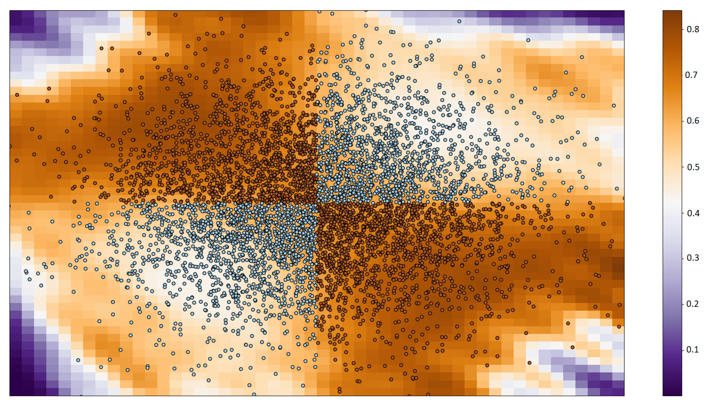
4.1. Classification
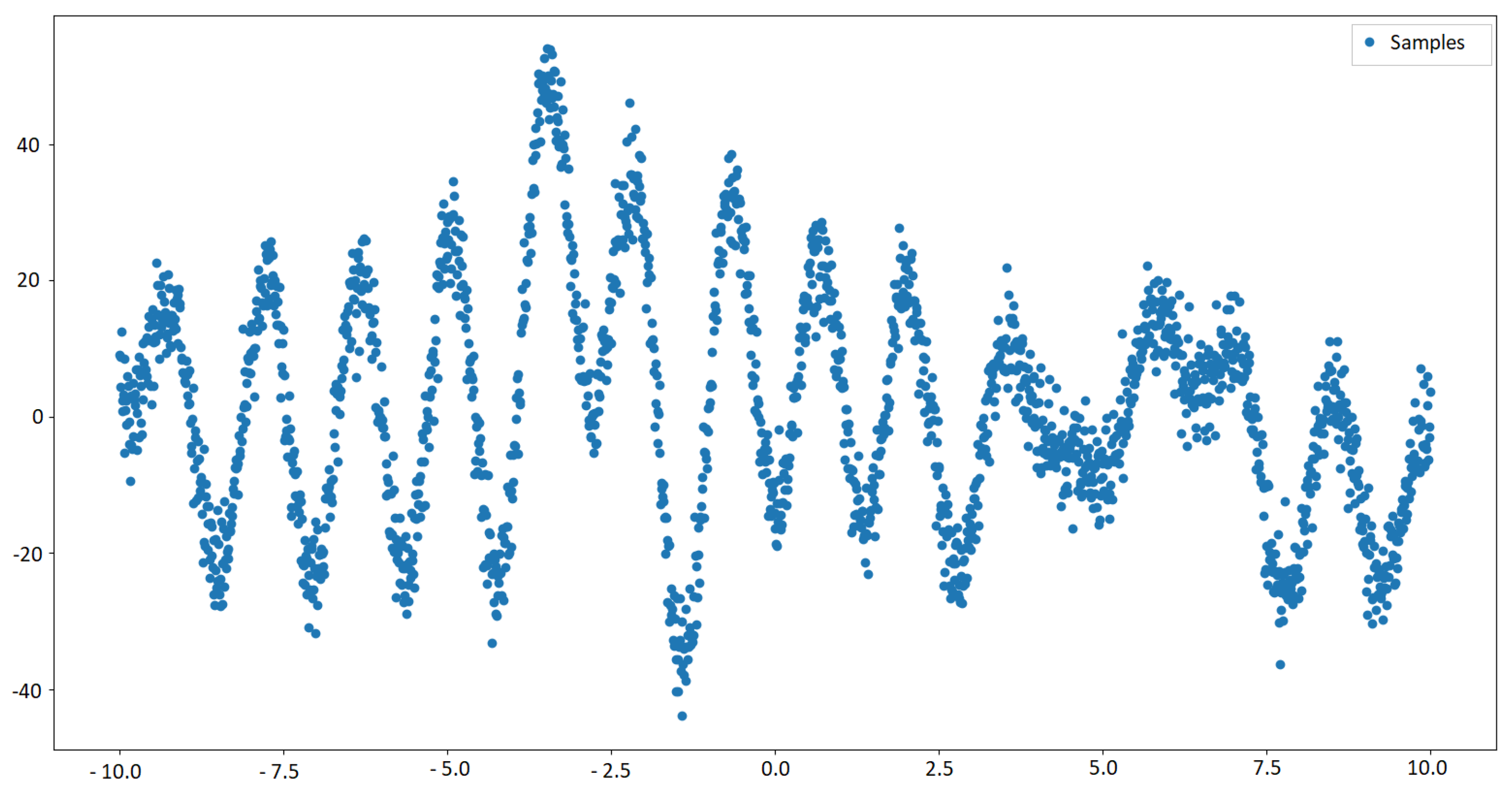
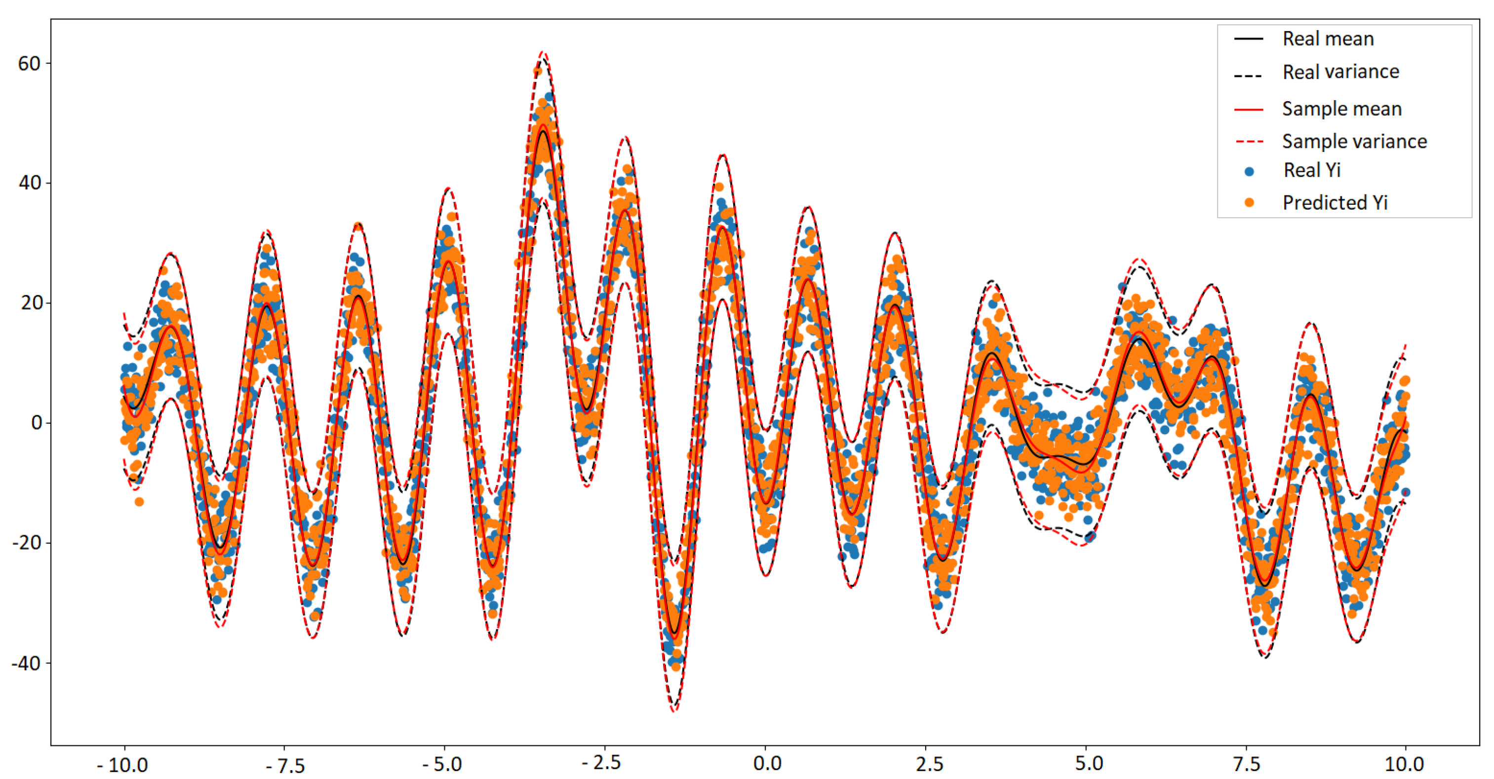
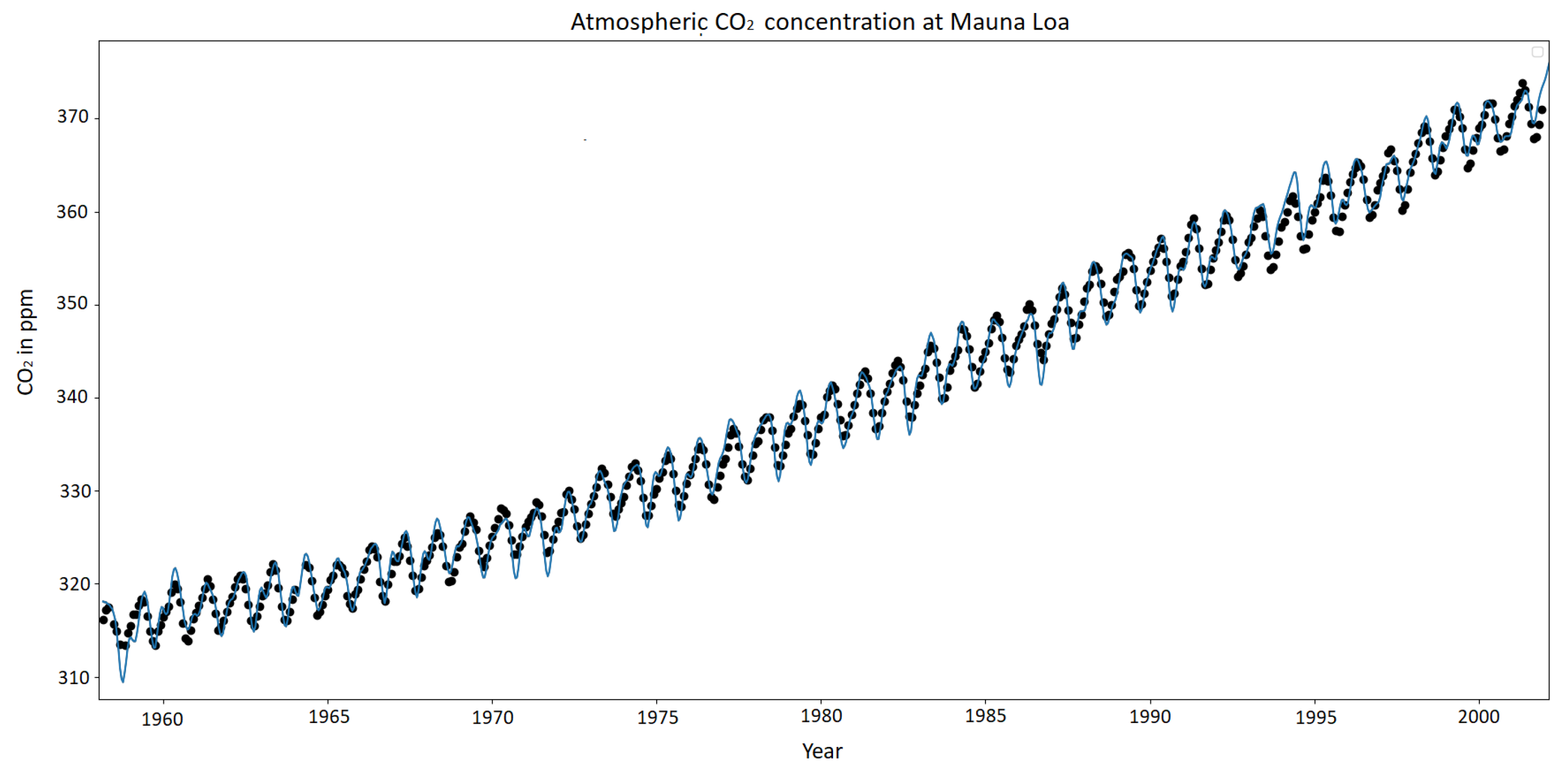
4.2. Regression
5. Conclusions
Author Contributions
Funding
Data Availability Statement
Acknowledgments
Conflicts of Interest
Abbreviations
| AUC | Area Under the Curve |
| MSE | Mean Squared Error |
| SVM | Support Vector Machine |
| Coefficient of determination | |
| MKL | Multiple Kernel Learning |
| SDP | Semi-Definite Programming |
| SMO | Sequential Minimal Optimization |
| BaNK | Bayesian Nonparametric Kernel |
| GaBaSR | Gaussian Mixture Bayesian Nonparametric Kernel Learning using Spectral Representation |
| GMM | Gaussian Mixture Model |
| MCMC | Markov Chain Monte Carlo |
| UCI | University of California, Irvine |
References
- Smola, A.J.; Schölkopf, B. Learning with Kernels; Citeseer: Princeton, NJ, USA, 1998; Volume 4. [Google Scholar]
- Soentpiet, R. Advances in Kernel Methods: Support Vector Learning; MIT Press: Cambridge, MA, USA, 1999. [Google Scholar]
- Anand, S.S.; Scotney, B.W.; Tan, M.G.; McClean, S.I.; Bell, D.A.; Hughes, J.G.; Magill, I.C. Designing a kernel for data mining. IEEE Expert 1997, 12, 65–74. [Google Scholar] [CrossRef]
- Schölkopf, B.; Smola, A.; Müller, K.R. Kernel principal component analysis. In Proceedings of the International Conference on Artificial Neural Networks, Lausanne, Switzerland, 8–10 October 1997; pp. 583–588. [Google Scholar]
- Zien, A.; Rätsch, G.; Mika, S.; Schölkopf, B.; Lengauer, T.; Müller, K.R. Engineering support vector machine kernels that recognize translation initiation sites. Bioinformatics 2000, 16, 799–807. [Google Scholar] [CrossRef] [PubMed]
- Tipping, M.E. The relevance vector machine. In Advances in Neural Information Processing Systems; MIT Press: Cambridge, MA, USA, 2000; pp. 652–658. [Google Scholar]
- Junli, C.; Licheng, J. Classification mechanism of support vector machines. In Proceedings of the WCC 2000-ICSP 5th International Conference on Signal Processing Proceedings 16th World Computer Congress, Beijing, China, 21–25 August 2000; Volume 3, pp. 1556–1559. [Google Scholar]
- Bennett, K.P.; Campbell, C. Support vector machines: Hype or hallelujah? Acm Sigkdd Explor. Newsl. 2000, 2, 1–13. [Google Scholar] [CrossRef]
- Gönen, M.; Alpaydın, E. Multiple kernel learning algorithms. J. Mach. Learn. Res. 2011, 12, 2211–2268. [Google Scholar]
- Lanckriet, G.R.; Cristianini, N.; Bartlett, P.; Ghaoui, L.E.; Jordan, M.I. Learning the Kernel Matrix with Semidefinite Programming. J. Mach. Learn. Res. 2004, 5, 27–72. [Google Scholar]
- Hoi, S.C.; Jin, R.; Lyu, M.R. Learning Nonparametric Kernel Matrices from Pairwise Constraints. In Proceedings of the 24th International Conference on Machine Learning ACM, Corvallis, OR, USA, 20–24 June 2007; pp. 361–368. [Google Scholar]
- Cvetkovic, D.M.; Doob, M.; Sachs, H. Spectra of Graphs; Academic Press: New York, NY, USA, 1980; Volume 10. [Google Scholar]
- Platt, J. Sequential Minimal Optimization: A Fast Algorithm for Training Support Vector Machines; Microsoft: Redmond, WA, USA, 1998. [Google Scholar]
- Bach, F.R.; Lanckriet, G.R.; Jordan, M.I. Multiple Kernel Learning, Conic Duality, and the SMO Algorithm. In Proceedings of the Twenty-First international Conference on Machine Learning ACM, Banff, AB, Canada, 4–8 July 2004; p. 6. [Google Scholar]
- Williams, C.K.; Rasmussen, C.E. Gaussian Processes for Machine Learning; MIT Press: Cambridge, MA, USA, 2006. [Google Scholar]
- Rahimi, A.; Recht, B. Random features for large-scale kernel machines. In Proceedings of the Advances in Neural Information Processing Systems, Vancouver, BC, Canada, 3–5 December 2007; pp. 1177–1184. [Google Scholar]
- Ghiasi-Shirazi, K.; Safabakhsh, R.; Shamsi, M. Learning translation invariant kernels for classification. J. Mach. Learn. Res. 2010, 11, 1353–1390. [Google Scholar]
- Oliva, J.B.; Dubey, A.; Wilson, A.G.; Póczos, B.; Schneider, J.; Xing, E.P. Bayesian Nonparametric Kernel-Learning. In Proceedings of the Artificial Intelligence and Statistics, Cadiz, Spain, 9–11 May 2016; pp. 1078–1086. [Google Scholar]
- Rasmussen, C. The infinite Gaussian mixture model. In Advances in Neural Information Processing Systems; MIT Press: Cambridge, MA, USA, 2000; pp. 554–560. [Google Scholar]
- Genton, M. Classes of kernels for machine learning: A statistics perspective. J. Mach. Learn. Res. 2001, 2, 299–312. [Google Scholar]
- Bochner, S. Harmonic Analysis and the Theory of Probability; California University Press: Berkeley, CA, USA, 1955. [Google Scholar]
- Silverman, R. Locally stationary random processes. IRE Trans. Inf. Theory 1957, 3, 182–187. [Google Scholar] [CrossRef]
- Hoeffding, W. Probability inequalities for sums of bounded random variables. In The Collected Works of Wassily Hoeffding; Springer: Berlin, Germany, 1994; pp. 409–426. [Google Scholar]
- Gelman, A.; Carlin, J.B.; Stern, H.S.; Dunson, D.B.; Vehtari, A.; Rubin, D.B. Bayesian Data Analysis; Chapman and Hall/CRC: Boca Raton, FL, USA, 2013. [Google Scholar]
- Geman, S.; Geman, D. Stochastic relaxation, Gibbs distributions, and the Bayesian restoration of images. IEEE Trans. Pattern Anal. Mach. Intell. 1984, 6, 721–741. [Google Scholar] [CrossRef] [PubMed]
- Dua, D.; Graff, C. UCI Machine Learning Repository. Open J. Stat. 2017, 10. [Google Scholar]
- Yeh, I.C.; Yang, K.J.; Ting, T.M. Knowledge discovery on RFM model using Bernoulli sequence. Expert Syst. Appl. 2009, 36, 5866–5871. [Google Scholar] [CrossRef]
- Gama, J. Electricity Dataset. 2004. Available online: http://www.inescporto.pt/~{}jgama/ales/ales_5.html (accessed on 6 August 2019).
- Carbon, D. Mauna LOA CO2. 2004. Available online: https://cdiac.ess-dive.lbl.gov/ftp/trends/CO2/sio-keel-flask/maunaloa_c.dat (accessed on 6 August 2019).
- Buitinck, L.; Louppe, G.; Blondel, M.; Pedregosa, F.; Mueller, A.; Grisel, O.; Niculae, V.; Prettenhofer, P.; Gramfort, A.; Grobler, J.; et al. API design for machine learning software: Experiences from the scikit-learn project. In Proceedings of the ECML PKDD Workshop: Languages for Data Mining and Machine Learning, Prague, Czech Republic, 23–27 September 2013; pp. 108–122. [Google Scholar]


| Dataset | N | M | Swaps | AUC |
|---|---|---|---|---|
| Breast Cancer [26] | 569 | 500 | 5 | 0.96480 |
| Credit-g [26] | 1000 | 500 | 5 | 0.44576 |
| Blood Transfusion [27] | 748 | 500 | 5 | 0.37572 |
| Electricity [28] | 45,312 | 500 | 5 | 0.68576 |
| Egg-eye-state [26] | 14,980 | 500 | 5 | 0.61635 |
| Kr vs Kp [26] | 3196 | 500 | 5 | 0.99357 |
| Dataset | N | M | Swaps | AUC |
|---|---|---|---|---|
| Breast Cancer [26] | 569 | 500 | 5 | 0.934656 |
| Credit-g [26] | 1000 | 500 | 5 | 0.85282 |
| Blood Transfusion [27] | 748 | 500 | 5 | 0 |
| Electricity [28] | 45,312 | 500 | 5 | 0.76076 |
| Egg-eye-state [26] | 14,980 | 500 | 5 | 0.692924 |
| Kr vs Kp [26] | 3196 | 500 | 5 | 0.96970 |
| Dataset | N | M | Swaps | AUC |
|---|---|---|---|---|
| Breast Cancer [26] | 569 | 500 | 5 | 0.51348 |
| Credit-g [26] | 1000 | 500 | 5 | 0.5142 |
| Blood Transfusion [27] | 748 | 500 | 5 | 0.54063 |
| Electricity [28] | 45,312 | 500 | 5 | 0.74991 |
| Egg-eye-state [26] | 14,980 | 500 | 5 | 0.519743 |
| Kr vs Kp [26] | 3196 | 500 | 5 | 0.9045 |
| Dataset | M | Swaps | MSE | |
|---|---|---|---|---|
| Mauna LOA CO | 250 | 5 | 0.60522 | 0.99789 |
| California houses | 250 | 5 | 2.91313 | −1.16892 |
| Boston house-price | 250 | 5 | 3.10931 | 0.97060 |
| Diabetes | 250 | 5 | 5,918,263.63330 | −869.13210 |
| Dataset | MSE | |
|---|---|---|
| Mauna LOA CO | 6.86 | 0.98 |
| California houses | 0.55 | 0.59 |
| Boston house-price | 18.92 | 0.78 |
| Diabetes | 3141.62 | 0.51 |
| Dataset | MSE | |
|---|---|---|
| Mauna LOA CO | 758.08513 | −1.60705 |
| California houses | 2.00777 | −0.50784 |
| Boston house-price | 47.66904 | 0.43533 |
| Diabetes | 8094.08752 | −0.36496 |
Disclaimer/Publisher’s Note: The statements, opinions and data contained in all publications are solely those of the individual author(s) and contributor(s) and not of MDPI and/or the editor(s). MDPI and/or the editor(s) disclaim responsibility for any injury to people or property resulting from any ideas, methods, instructions or products referred to in the content. |
© 2023 by the authors. Licensee MDPI, Basel, Switzerland. This article is an open access article distributed under the terms and conditions of the Creative Commons Attribution (CC BY) license (https://creativecommons.org/licenses/by/4.0/).
Share and Cite
Pena-Llamas, L.R.; Guardado-Medina, R.O.; Garcia, A.; Mendez-Vazquez, A. Kernel Learning by Spectral Representation and Gaussian Mixtures. Appl. Sci. 2023, 13, 2473. https://doi.org/10.3390/app13042473
Pena-Llamas LR, Guardado-Medina RO, Garcia A, Mendez-Vazquez A. Kernel Learning by Spectral Representation and Gaussian Mixtures. Applied Sciences. 2023; 13(4):2473. https://doi.org/10.3390/app13042473
Chicago/Turabian StylePena-Llamas, Luis R., Ramon O. Guardado-Medina, Arturo Garcia, and Andres Mendez-Vazquez. 2023. "Kernel Learning by Spectral Representation and Gaussian Mixtures" Applied Sciences 13, no. 4: 2473. https://doi.org/10.3390/app13042473