Article

Generative Music with Partitioned Quantum Cellular Automata

by
Eduardo Reck Miranda
1,2,* and
Hari Shaji
1
1
Interdisciplinary Centre for Computer Music Research (ICCMR), University of Plymouth, Plymouth PL4 8AA, UK
2
Quantinuum, Partnership House, Carlisle Place, London SW1P 1BX, UK
*
Author to whom correspondence should be addressed.
Appl. Sci. 2023, 13(4), 2401; https://doi.org/10.3390/app13042401
Submission received: 3 January 2023 / Revised: 31 January 2023 / Accepted: 3 February 2023 / Published: 13 February 2023
(This article belongs to the Special Issue Algorithmic Music and Sound Computing)

Abstract

:
Cellular automata (CA) are abstract computational models of dynamic systems that change some features with space and time. Music is the art of organising sounds in space and time, and it can be modelled as a dynamic system. Hence, CA are of interest to composers working with generative music. The art of generating music with CA hinges on the design of algorithms to evolve patterns of data and methods to render those patterns into musical forms. This paper introduces methods for creating original music using partitioned quantum cellular automata (PQCA). PQCA consist of an approach to implementing CA on quantum computers. Quantum computers leverage properties of quantum mechanics to perform computations differently from classical computers, with alleged advantages. The paper begins with some explanations of background concepts, including CA, quantum computing, and PQCA. Then, it details the PQCA systems that we have been developing to generate music and discusses practical examples. PQCA-generated materials for Qubism, a professional piece of music composed for London Sinfonietta, are included. The PQCA systems presented here were run on real quantum computers rather than simulations thereof. The rationale for doing so is also discussed.

1. Introduction

In this paper, we report on our research into harnessing quantum computing for creating original music.
The great majority of research in artificial intelligence (AI) for musical composition has been focused on developing systems for imitating the style of existing music [1]. For instance, ref. [2] introduced a system that analysed given pieces of music and recombined the identified musical elements into new pieces, which sounded like the originals. This system used a recombination algorithm informed by augmented transition networks (ATN). These were originally developed for linguistics to analyse the structure of sentences [3]. More recently, ref. [4] introduced a system based on deep learning neural networks [5] to compose tunes imitating the ones used for training the network. An overview of deep learning models for music composition is available in [6].
Indeed, state-of-the-art AI is capable of generating convincing musical compositions [1,7]. However, the work reported here is not aimed at systems to imitate existing repertoires. We are interested in developing AI technology to support the creation of innovative music instead. Examples of previous work in this vein are sparse. A notable system, Fractal Music [8], generates music from fractals [9]. Moreover, [10] introduced CAMUS, a system that generated music using cellular automata (CA) [11]. This system inspired the development of the systems reported in the present paper.
Quantum computing is an emergent technology, which is advancing rapidly. It promises a number of advantages for certain computational tasks, which current digital processors struggle to realize. For instance, the simulation of molecules for drug discovery and development is computationally very demanding, even for current supercomputers. Quantum computing brings new approaches to optimise this, which will enable drugs to be developed faster and more effectively [12].
For music, quantum computers will bring considerable processing speed and capacity to handle increased quantities of data simultaneously. This is bound to impact future music recommendation systems [13]. Furthermore, and perhaps more significantly, this new technology is bound to foster new approaches to making music, which would be unlikely otherwise. For instance, whereas ref. [14] developed a quantum computing music sampler called QuiKo, ref. [15] developed the concept of a Qeyboard, a quantum musical instrument. Moreover, [16] developed Quantum Music Playground, an educational tool for learning quantum computing concepts through music. This paper introduces a system for composing music using partitioned quantum cellular automata (PQCA) [17]. It follows from preliminary work introduced in [18].
Music is the art of organising sounds in space and time [19,20]. CA are abstract computational models of systems that change some features with space and time [11]. Pragmatically, CA models are useful because they generate patterns of data that can be translated into music [21,22,23]. Quantum versions of CA have been developed to simulate quantum mechanical phenomena; e.g., quantum lattice gases [24], hence our rationale for exploring PQCA to generate music.
We begin with a brief explanation of quantum computing, CA and quantum CA. Then, we present the new PQCA models that we developed for musical composition and show practical examples produced for a musical composition entitled Qubism We end the paper with concluding remarks and directions for further development.

2. Background

2.1. Cellular Automata (CA)

CA are discrete dynamical systems often described as counterparts to partial differential equations, which are suitable for modelling continuous dynamical systems. CA have been used to model phenomena in a variety of fields, including image processing [25], ecology [26], biology [27], sociology [28] and vocal production [29].
Stanislaw Ulam and John von Neumann conceived the notion of CA in the 1960s [30]. They were looking into developing self-reproducing machines. They built a model consisting of a grid of cells. Each cell could assume several values representing the components from which they built an abstract self-reproducing machine. Completely controlled by a set of simple rules, the machine was able to make identical copies of itself at other locations on the grid.
In practice, a CA model is often implemented as an arrangement of identical cells that influence one another. This arrangement usually forms either a one-dimensional bar or a two-dimensional grid of cells, respectively. However, in theory, there could be any number of dimensions. An algorithm expressing transition rules operates on all cells simultaneously to alter their values. The transition rules take into account the values of cells that are next to or surrounding each cell.
The number of possible values for the cells might simply be the two numbers one and zero (e.g., representing on and off switches), but it can be any amount. Cell values can represent objects, properties or processes, depending on what is being modelled. For instance, if each cell stands for a portion of a landscape, then a certain value might represent the type of vegetation that is growing in the area.
The functioning of a CA-based system is normally monitored on a computer screen as a sequence of changing patterns, following the tick of a virtual clock, like in an animated film.
Figure 1 shows an example consisting of a bar of cells, each of which can have the value either zero or one, represented by the colours white or black, respectively. From a given overall initial configuration of values, all cells change simultaneously at each tick t of the virtual clock.
An example of two-dimensional CA, known as Conway’s Game of Life [31], is shown in Figure 2. The system CAMUS, mentioned earlier, uses Game of Life to generate music [10].

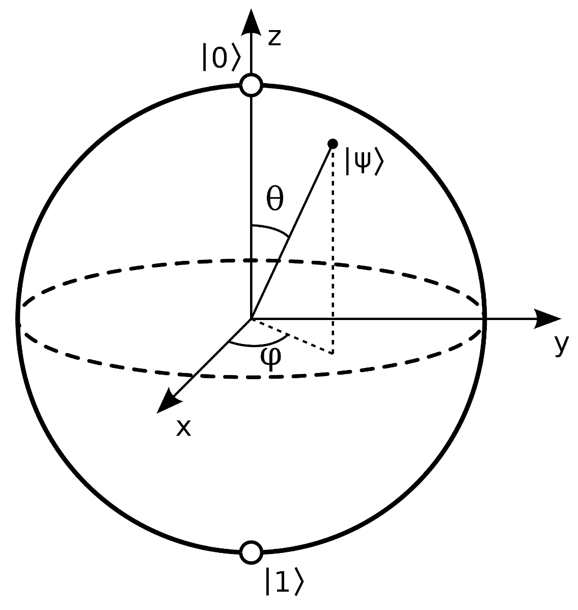
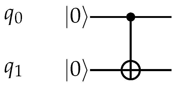
2.2. Quantum Computing

The basic unit for representing information in a quantum computer is the qubit. A qubit is to a quantum computer what a bit is to a digital computer. However, qubits operate at the atomic or even subatomic level. Therefore, they are subject to the laws of quantum mechanics, with their properties of superposition and entanglement. In quantum mechanics, an object does not exist in a determined state. Its state is unknown until one observes it.
The state of a qubit lives in a two-dimensional complex vector space, referred to as a two-dimensional Hilbert space. The canonical basis vectors in a Hilbert space are notated as | 0 and | 1 . This notation, referred to as the Dirac notation, provides an abbreviated way to represent a vector. For instance, | 0 and | 1 represent the vectors shown in Equation (1):
| 0 = 1 0 and | 1 = 0 1
The general state | ψ of a qubit is written as a linear combination of the basis vectors as follows: | ψ = α | 0 + β | 1 with α , β C and | α | 2 + | β | 2 = 1 . This linear combination expresses a state of superposition.
In a nutshell, qubits process information in a state of superposition. However, they will return binary numbers (zeros and ones) when we read them. In quantum computing terminology, the act of reading qubits is referred to as projective measurement.
Not expressed in the equation for | ψ above, however, is the phase of the qubit. To visualize this, let us consider a single qubit as a transparent sphere with opposite poles. From its centre, the vector | ψ can point to anywhere on the surface. This sphere is called the Bloch sphere and the vector is referred to as a state vector (Figure 3). The angle φ defines the phase.
Quantum computers are programmed by applying sequences of unitary linear operations U to state vectors: | ψ = U | ψ . Programming languages for quantum computing provide a number of such linear operators, referred to as gates. For instance, the X gate rotates the state vector by 180 degrees around the x-axis of the Bloch sphere. Thus, if the qubit vector is pointing to | 0 , then this gate flips it to | 1 : | 1 = X | 0 , and vice versa, | 0 = X | 1 .
A parametric rotation Rx ( θ ) gate is typically available for quantum programming, where the angle for the rotation around the x-axis is specified. Similarly, there are Rz ( φ ) and Ry ( θ ) gates for rotations on the z-axis and y-axis of the Bloch sphere.
Mathematically, quantum gates are represented as matrices. For instance, the X gate, which flips the state of a qubit is represented as shown in Equation (2). In this case, gate operation is represented mathematically as the multiplication of a matrix (gate) by a vector (qubit state).
X = 0 1 1 0
Thus, the application of an X gate to | 0 is written as shown in Equation (3):
X ( | 0 ) = 0 1 1 0 × 1 0 = 0 1 = | 1
An important gate for quantum computing is the Hadamard gate, referred to as the H gate. It has the matrix shown in Equation (4).
H = 1 2 1 2 1 2 1 2 = 1 2 1 1 1 1
The application of the H gate to a qubit pointing to | 0 puts it in superposition, right at the equator of the Bloch sphere. That is, it puts the qubit into a balanced superposition state consisting of an equal-weighted combination of two opposing states, where α 2 = 0.5 and β 2 = 0.5 . This is depicted in Equation (5):
H ( | 0 ) = 1 2 ( | 0 + | 1 )
Gates can also operate on multiple qubits. For instance, the controlled X gate (also known as CX or CNOT gate) puts two qubits in entanglement. The CX gate applies an X gate on a qubit only if the state of another qubit is | 1 . Thus, this gate establishes a dependency (or a correlation) of the state of one qubit with the value of another (Figure 4).
In practice, any quantum gate can be made conditional, and entanglement can take place between more than two qubits.
Quantum processing with multiple qubits is represented using tensored vectors. A tensored vector is the result of the tensor product (represented by the symbol ⨂) of two or more vectors. A system of two qubits looks like | 0 | 0 , but it is normally abbreviated to | 00 . It is useful to study the expanded form of the tensor product to follow how it works. For instance, see Equation (6).
| 01 = | 0 | 1 = 1 0 0 1 = 1 × 0 1 × 1 0 × 0 0 × 1 = 0 1 0 0
Furthermore, let us consider two qubits | q 1 and | q 0 with state vectors | Ψ and | Φ , respectively. These are shown in Equation (7). Moreover, Equation (8) describes a system with two qubits | q 1 and | q 0 , combining the state vectors | Ψ and | Φ .
| Ψ = α | 0 + β | 1 for q 0 | Φ = γ | 0 + δ | 1 for q 1
| Ψ | Φ = α γ | 00 + α δ | 01 + β γ | 10 + β δ | 11
In fact, Equation (8) represents a new quantum state with four amplitude coefficients (Equation (9)). Thus, Equation (10) expresses that each of the four quantum states has an equal probability of 25% each of being returned.
| Ω = ω 0 | 00 + ω 1 | 01 + ω 2 | 10 + ω 3 | 11
| Ω = 1 4 | 00 + 1 4 | 01 + 1 4 | 10 + 1 4 | 11
Now, it should be straightforward to work out how to describe quantum systems with more qubits. For instance, Equation (11) depicts a quantum system with four qubits:
| B = β 0 | 0000 + β 1 | 0001 + β 2 | 0010 + β 3 | 0011 + β 4 | 0100 + β 5 | 0101 + β 6 | 0110 + β 7 | 0111 + β 8 | 1000 + β 9 | 1001 + β 10 | 1010 + β 11 | 1011 + β 12 | 1100 + β 13 | 1101 + β 14 | 1110 + β 15 | 1111
A linear increase in the number of qubits extends the capacity of representing information on a quantum computer exponentially [32]. With a quantum system composed of n qubits, their joint state space is given by the tensor product of their individual state spaces and has dimension 2 n . With qubits in superposition, a quantum computer can consider all possible values of some input data simultaneously.
The evolution of many qubits interacting with each other is given by a global exponentially large unitary operator acting on the entire joint exponentially large state space. The larger this space, the harder for classical computers to process; hence, in principle, the advantage of quantum computers over digital classical ones.
A quantum program is often depicted as a circuit with sequences of quantum gates operating on qubits (Figure 5). Typically, the qubits start in the state | 0 . When the qubits are read, the results can be stored in standard digital memory, which is accessible for further handling.
Quantum algorithms require a different way of thinking from the way one normally approaches programming. For instance, it is not possible to store quantum states in a “working memory” (classically) for access later in the algorithm. This is due to the so-called non-cloning principle of quantum mechanics, which states that it is impossible to create an independent and identical copy of an arbitrary unknown quantum state. For an in-depth theoretical introduction to quantum computing, please refer to [32,33,34].

3. Partitioned Quantum Cellular Automata

Quantum cellular automata (QCA), as its name suggests, are CA for quantum computers. Actually, they were introduced as an alternative paradigm for quantum computation and were shown to be universal: QCA can function as a quantum Turing machine. Please, refer to [35] for a theoretical discussion about QCA and universal computation.
In QCA, the cells are implemented as qubits. However, implementing a QCA with currently available quantum hardware is not trivial. The difficulty lies in updating all cells, or qubits, at the same cycle. For instance, if we attempt to implement a quantum version of any classical CA algorithm, we would need to store a copy of the original state of a qubit to update the others. However, this is not allowed with a quantum computer because of the non-cloning principle mentioned earlier [32].
A number of approaches have been proposed to get around the difficulty mentioned above [35]. One of them is referred to as partitioned quantum cellular automata (PQCA) [17,36].
This section introduces the basics of PQCA. For a rigorous theoretical discussion please refer to [17,36], in particular, to learn more about their nonclassical behaviour. Here, we focus on the practical aspects of implementing PQCA.
To recapitulate, a CA at a certain time t is characterized by two properties: its current state and an update step that establishes the values of the cells at time t + 1 . Thus, we need to apply an update circuit to all qubits of the automaton simultaneously at each time step.
In PQCA, we first define one or more partition schemes to split an arrangement of cells into tessellating supercells. Then, a global update circuit is built from update frames. These update frames are defined using the partitions and local circuits.

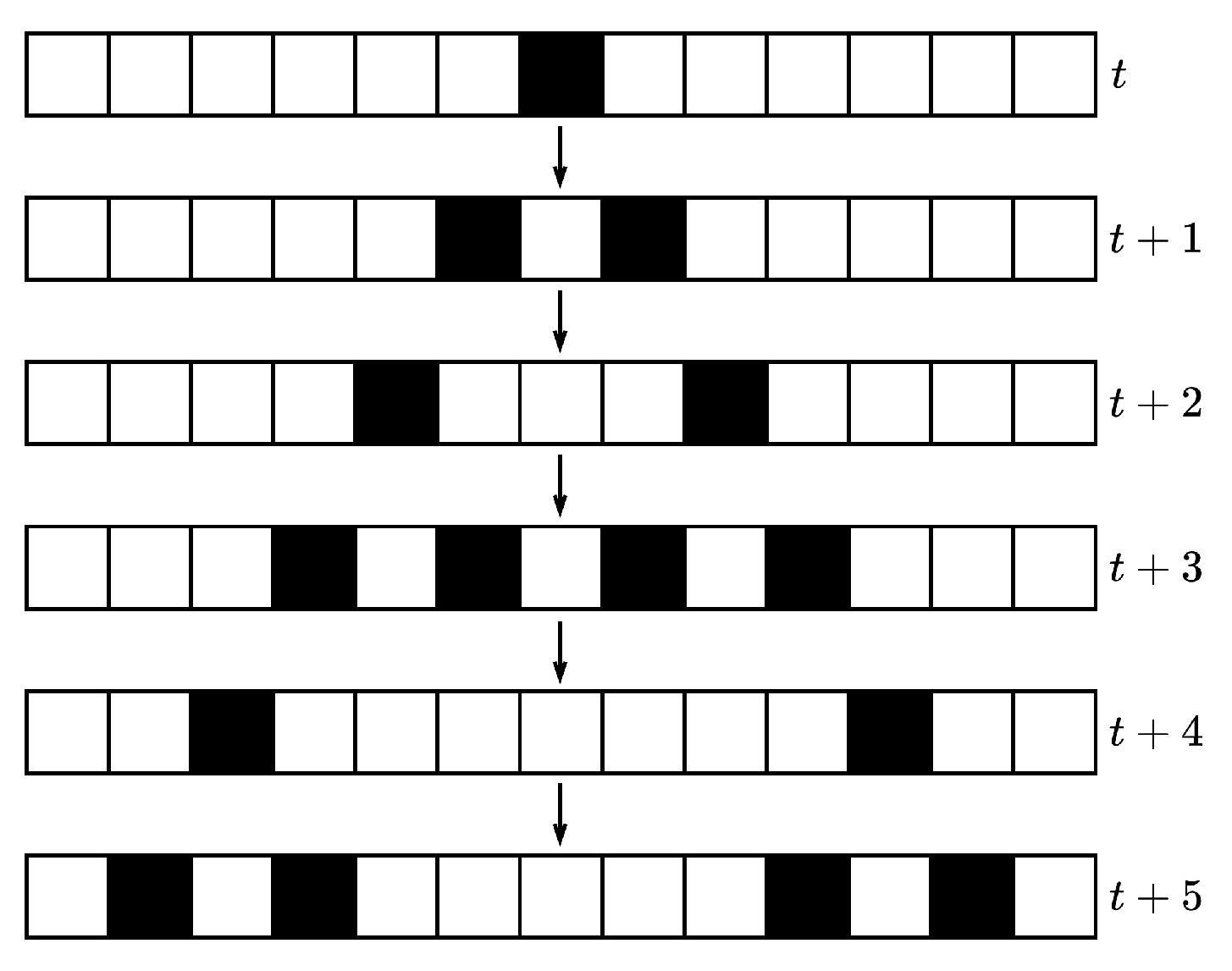
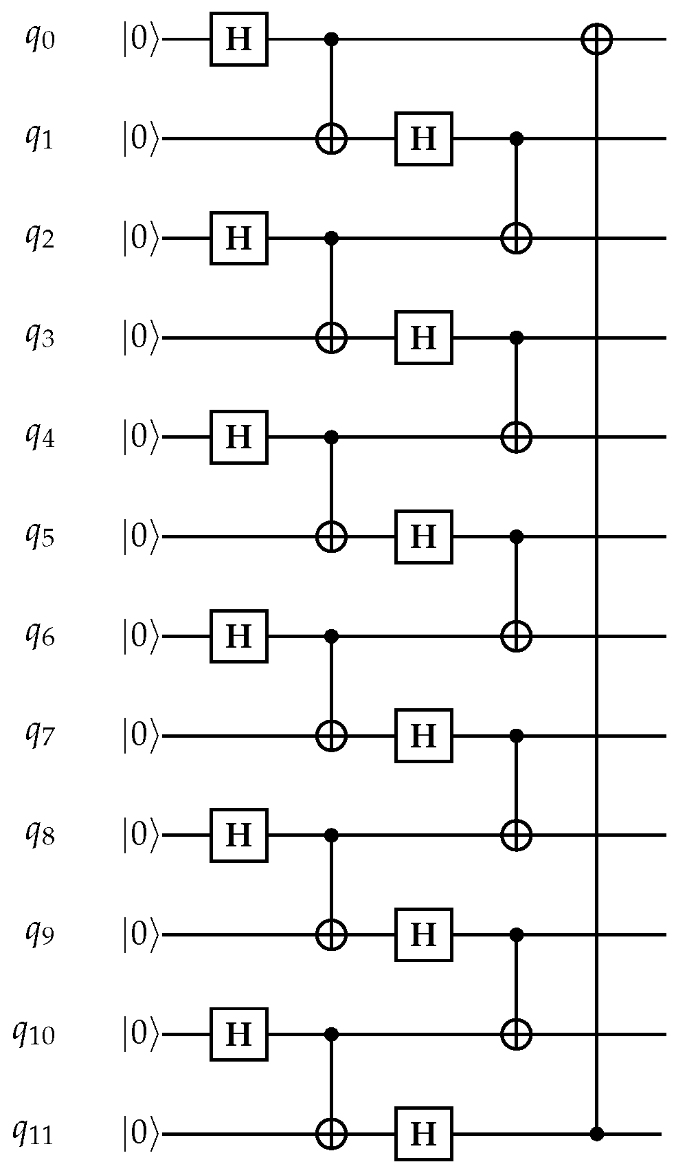
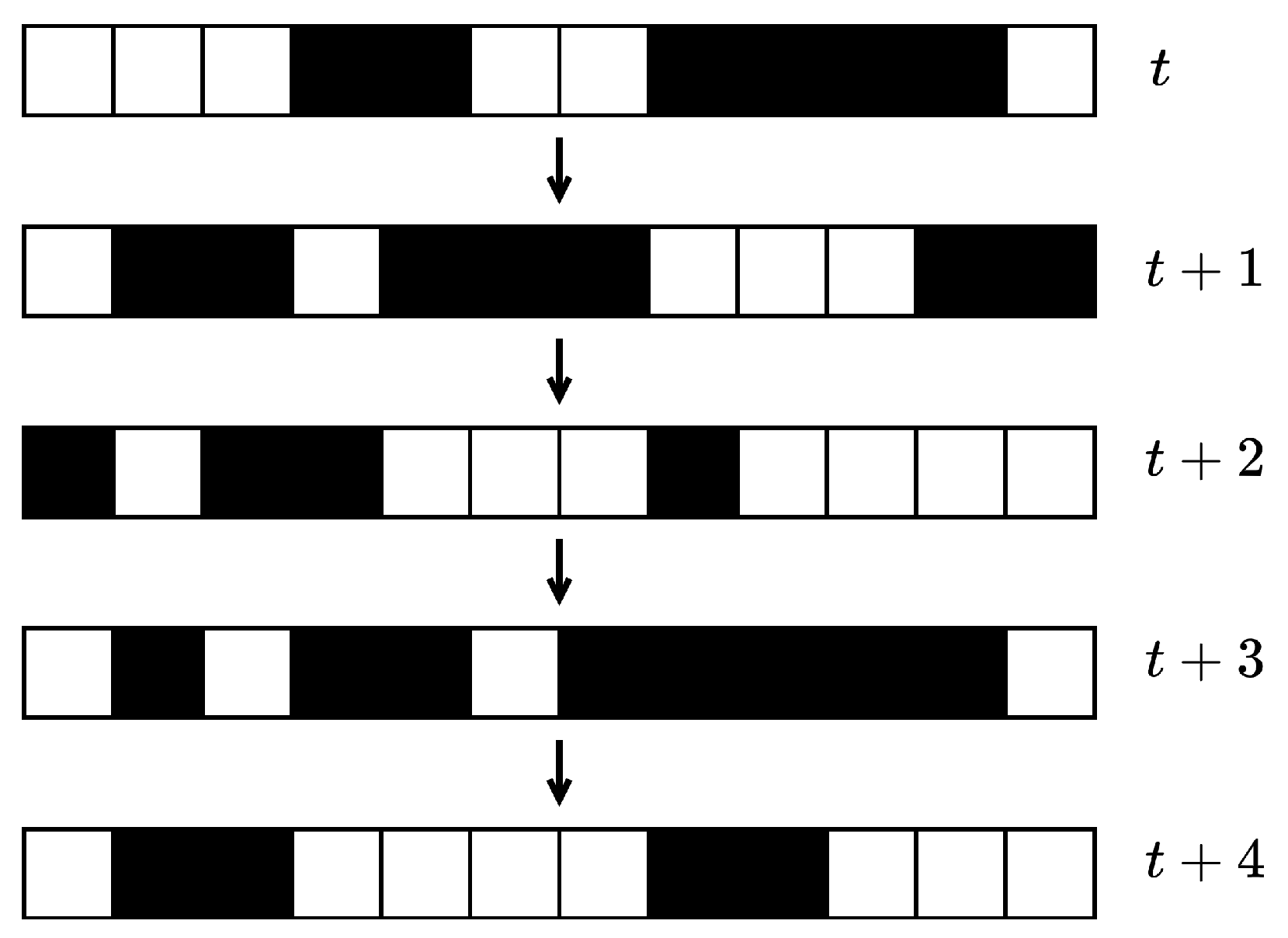
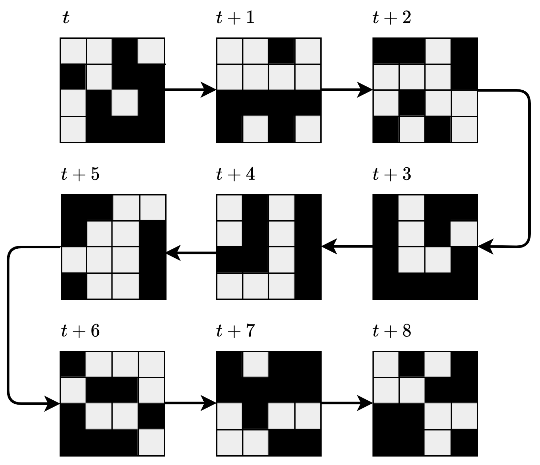
3.1. One-Dimensional PQCA

As an example, consider a one-dimensional PQCA characterised by a bar of twelve cells. This is depicted in Figure 6.
Figure 7 shows two examples of partition schemes. At the top is a partition consisting of six supercells, two cells long each. Let us notate this as follows:
{ [ 1 , 2 ] , [ 3 , 4 ] , [ 5 , 6 ] , [ 7 , 8 ] , [ 9 , 10 ] , [ 11 , 12 ] }
At the bottom is a shifted version of the partition:
{ [ 2 , 3 ] , [ 4 , 5 ] , [ 6 , 7 ] , [ 8 , 9 ] , [ 10 , 11 ] , [ 12 , 1 ] }
Let us define a local circuit for the one-dimensional PQCA considering the partitions shown in Figure 7. A local circuit needs to have the same number of qubits as the number of cells in the target supercells. In this case, we are working with supercells that are two cells long each. Therefore, the local update circuit must work with two qubits. Figure 8 shows a two-qubit circuit, with a H and a CX gate, respectively. This local circuit is then tessellated through the supercells forming an update frame.
A global update circuit can and should include more than one update frame. Figure 9 shows an example of a global update circuit using two update frames, one based on the partition shown at the top of Figure 7 and the other using a shifted version of the partition, which is shown at the bottom of the figure. For this example, we used the same local circuit for both update frames, but we could have used two distinct local circuits instead.
An example showing four cycles of the PQCA from given initial cell values—or qubit states—is shown in Figure 10. The automaton applies the global update circuit to the current qubit states, and the measured output is used to set the qubits with states for the next cycle and so on.

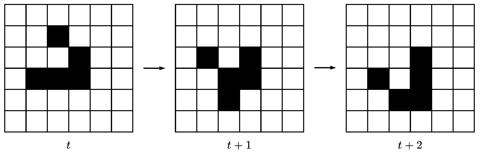
3.2. Two-Dimensional PQCA

As an example of a two-dimensional PQCA, let us consider a 4 × 4 grid of cells, as shown in Figure 11.
Figure 12 and Figure 13 show two examples of partitions: one is a partition of the grid into horizontal strips, and the other into vertical strips, respectively. Effectively, Figure 12 constitutes eight supercells, each of which is formed by two cells. In addition, Figure 13 has four supercells, each of which is formed by four cells.
In the same spirit of one-dimensional PQCA, let us define a global update circuit for the two-dimensional PQCA shown in Figure 11.
For this example, we defined two local circuits, one for each of the partitions. Figure 14 and Figure 15 show the local circuits for the partitions in Figure 12 and Figure 13, respectively. They yield two update frames, which combined result in the global update circuit with 16 qubits, as shown in Figure 16. An example of a pattern produced by this two-dimensional PQCA is shown in Figure 17.

4. Music Mapping

The art of generating music with CA hinges on the methods to convert their outputs into patterns of musical notes. It is here that composers can experiment with different mapping designs. An example developed to make music with the Game of Life CA (shown in Figure 2) is discussed in [10]. A preliminary mapping design for PQCA was presented in [18].
This section presents the mapping schemes developed to generate musical forms for a piece for a chamber ensemble, composed for London Sinfonietta, entitled Qubism.
We developed two distinct mapping schemes: one for the one-dimensional and another for the two-dimensional PQCA, respectively.

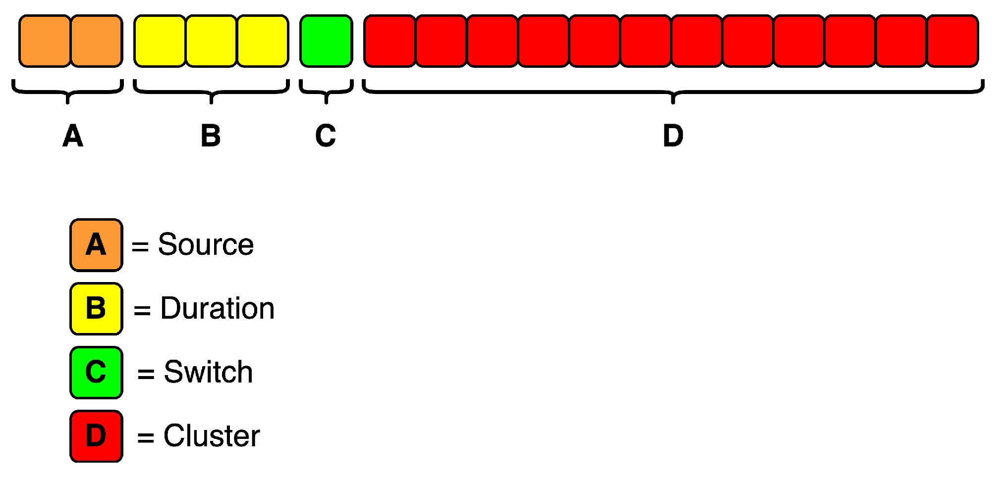
4.1. One-Dimensional PQCA Mapping

A bar of 18 cells forms the one-dimensional PQCA. The mapping scheme generates clusters of musical notes. Each cycle of the PQCA produces an eighteen-bit long bitstring, which is converted into either a cluster or a rest (i.e., silence).
A cluster is a group of notes that are played simultaneously. It can have up to 12 notes. Conversely, a rest is when a cycle does not generate any notes at all.
To encode musical information, the bitstring is split into four sections (Figure 18). Each section forms a code representing a property of the cluster, as follows (the bit order is from the left to the right of the bitstring):
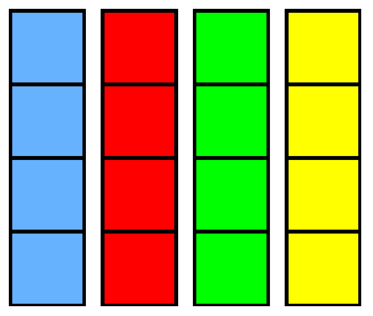
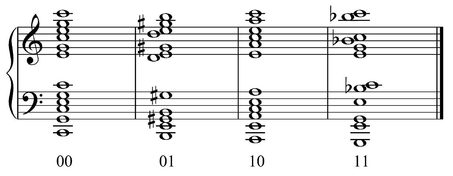
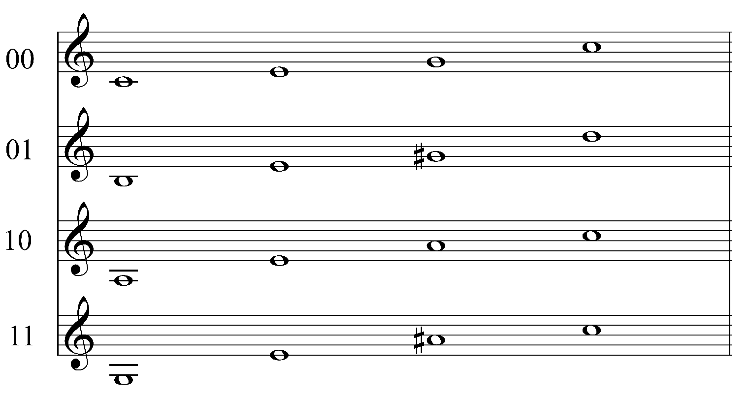
  • Code A (bits 1 and 2) defines the source of the notes. There are four different sources to choose from (Figure 19).
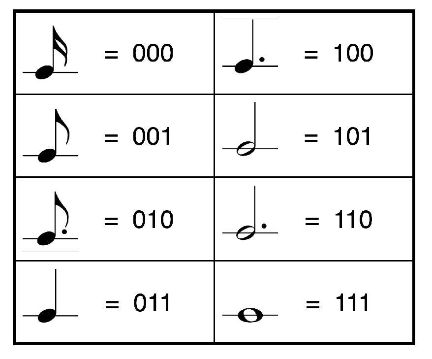
  • Code B (bits 3, 4 and 5) defines the duration of the cluster. There are eight different durations to choose from (Figure 20).
  • Code C (bit 6) = rest switch.
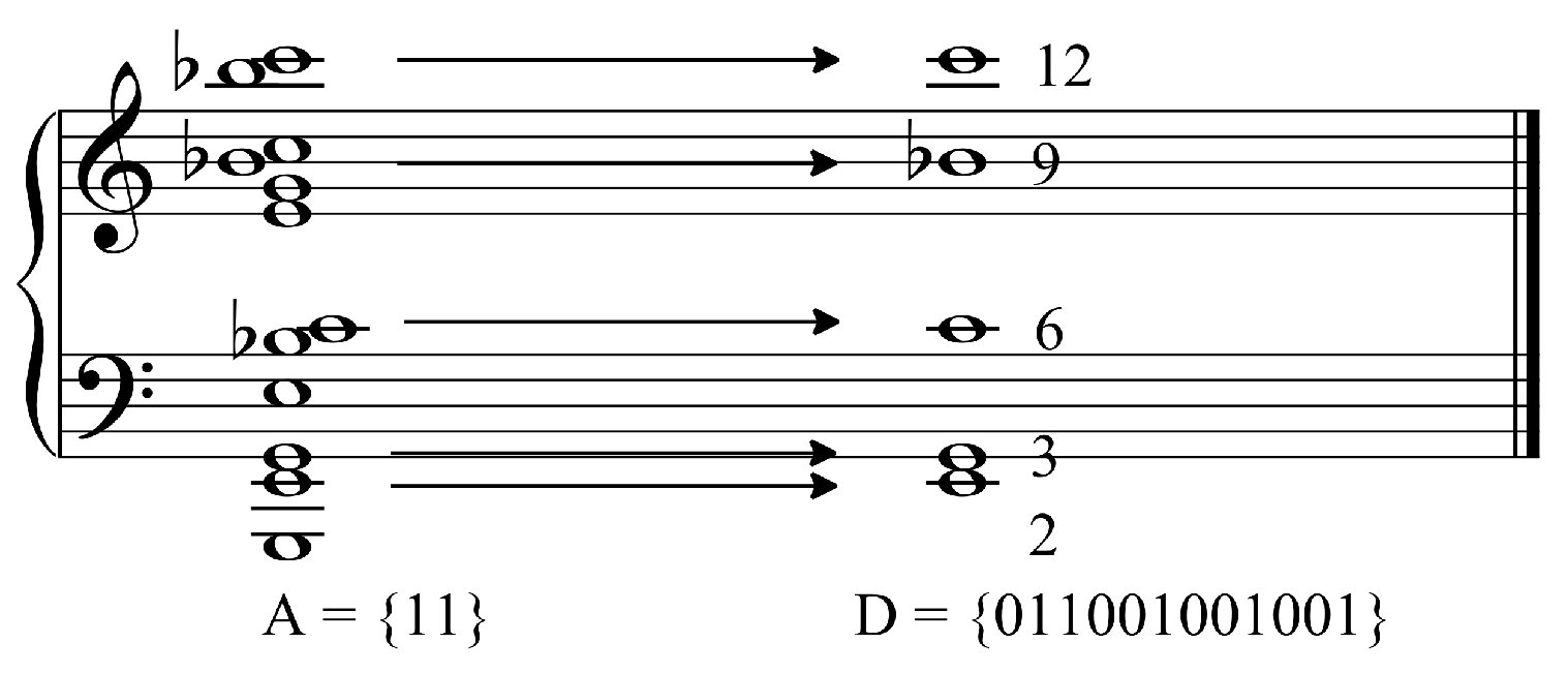
  • Code D (bits from 7 to 18) defines the notes of the cluster; these notes are picked from the source defined by code A
The pitches for a cluster are picked from one of four sources, according to code A. Hence, this code requires two bits to encode four options. The sources can be customised. The composition Qubism used two sets of sources, one of which is shown in Figure 19.
There are eight options for the duration of a cluster, which are defined by code B (Figure 20). It requires three bits to encode eight options. Moreover, code C establishes if the respective cluster is active (code C = 1 ) or constitutes a rest (code C = 0 ).
Note that in Figure 19, the sources are already displayed as clusters of twelve pitches. Formed by the last twelve bits of the bitstring (from 7 to 18), code D defines which notes in the selected source will constitute the resulting cluster.
The positions of digits “1” in the string (from the left to the right) correspond to the positions of the notes to be picked from the source (from the bottom to the top). For instance, let us consider code D = { 011001001001 } . This instructs the system to pick the second, third, sixth, ninth and twelfth notes to form the cluster, as illustrated in Figure 21. However, if code C = 0 , then the system would output a rest, respective to the duration of the cluster instead. A real example is discussed in Section 5.

4.2. Two-Dimensional PQCA Mapping

The mapping scheme for the two-dimensional PQCA generates polyphonic musical segments to be played by an ensemble of instruments.
The PQCA grid should be thought of as a structural frame for a musical segment, and the values of the cells specify how the contents are arranged in the frame.
The vertical dimension of the grid defines the number of instruments. The horizontal dimension defines the length of the segment and encodes a transposition coefficient, which is explained below. As a default, the scheme is set to associate each column of the grid to a beat in a 4/4 measure; this is customisable.
As an example, consider the 8 × 4 grid of cells depicted in Figure 22. Let us hypothesise that this is the output from one PQCA cycle. This grid provides a frame for two 4/4 measures. That is, each cycle of the PQCA will generate two measures of music at a time. Moreover, in this case, the music will be for four instruments. This particular example yields three notes: there are three cells that are equal to 1. Two notes are played by instrument number three and one note by instrument number two. How are the pitches, placements and durations of the notes calculated?
Just as in the one-dimensional PQCA mapping (Section 4.1), here we also have sources of pitches (Figure 23) and codes for durations (Figure 24).

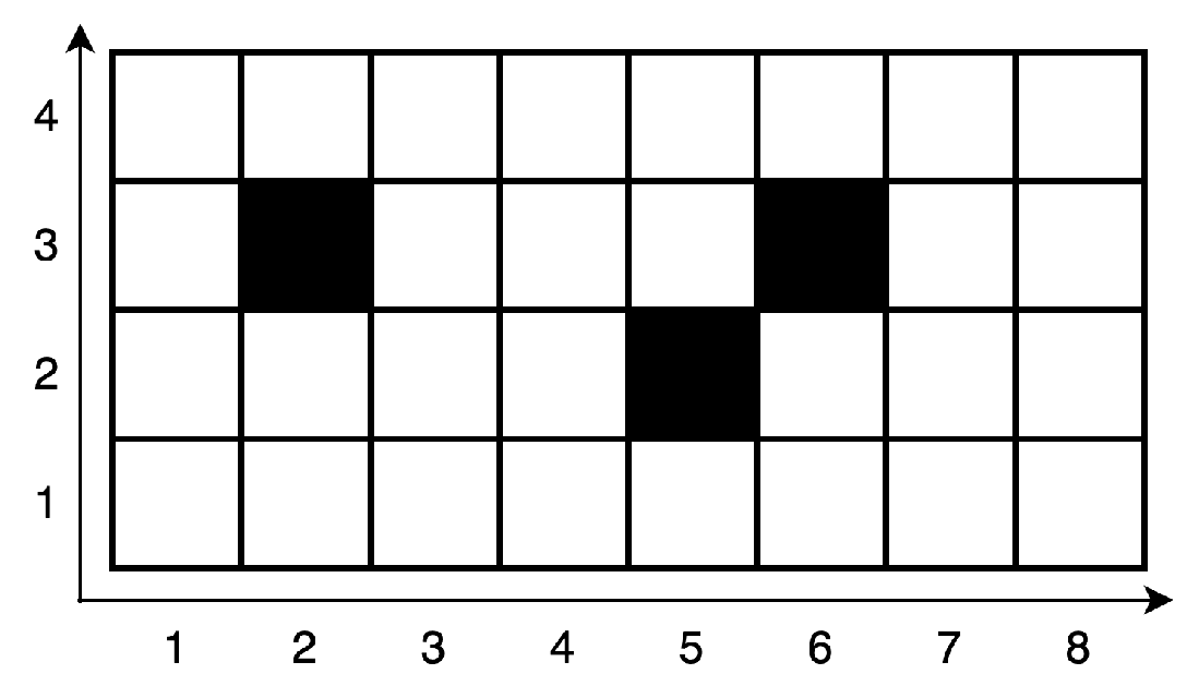
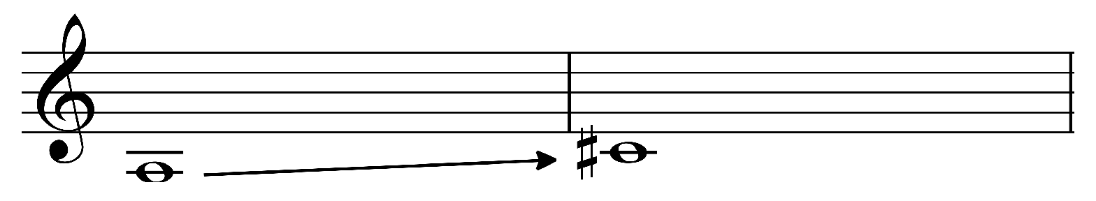
4.2.1. Calculating the Pitch of a Cell

The system is programmed with four sources of reference pitches, labelled as 00, 01, 10 and 11, respectively (Figure 23). The sources can hold any number of pitches. In this example, they hold four pitches each.
To establish which source to pick a reference pitch from, the system builds a two-bit long code ( x y ) with the values of the top right (x) and bottom left (y) neighbours of the respective cell (Figure 25). For instance, in Figure 22, the cell at coordinates ( 5 , 2 ) yields the code ( 10 ) : x = 1 and y = 0 . Thus, the system retrieves the first pitch, A 3 , from source 10. The system loops through a source sequentially; the next time it needs to retrieve a reference pitch from source 10, it will pick the second one, E 4 , and so on.
In addition to the sources, the system holds a list of transposition coefficients Δ = [ δ 1 , δ 2 , , δ n ] . These coefficients correspond to semitones for transposing a given reference pitch. That is, the system transposes the selected reference pitch by adding to (or subtracting from) a transposition coefficient δ .
Let us consider the following example: Δ = [ 7 , 5 , 0 , 12 , 4 , 0 , 5 , 7 ] . Δ must be of the same length as the horizontal dimension of the grid; in this case, equal to eight. This is because the x coordinate of the cell defines the index i of Δ [ i ] to retrieve the respective coefficient to transpose the pitch. Thus, for cell ( 5 , 2 ) , it will add four semitones ( Δ [ 5 ] = 4 ) to pitch A 3 , resulting in C 4 (Figure 26).

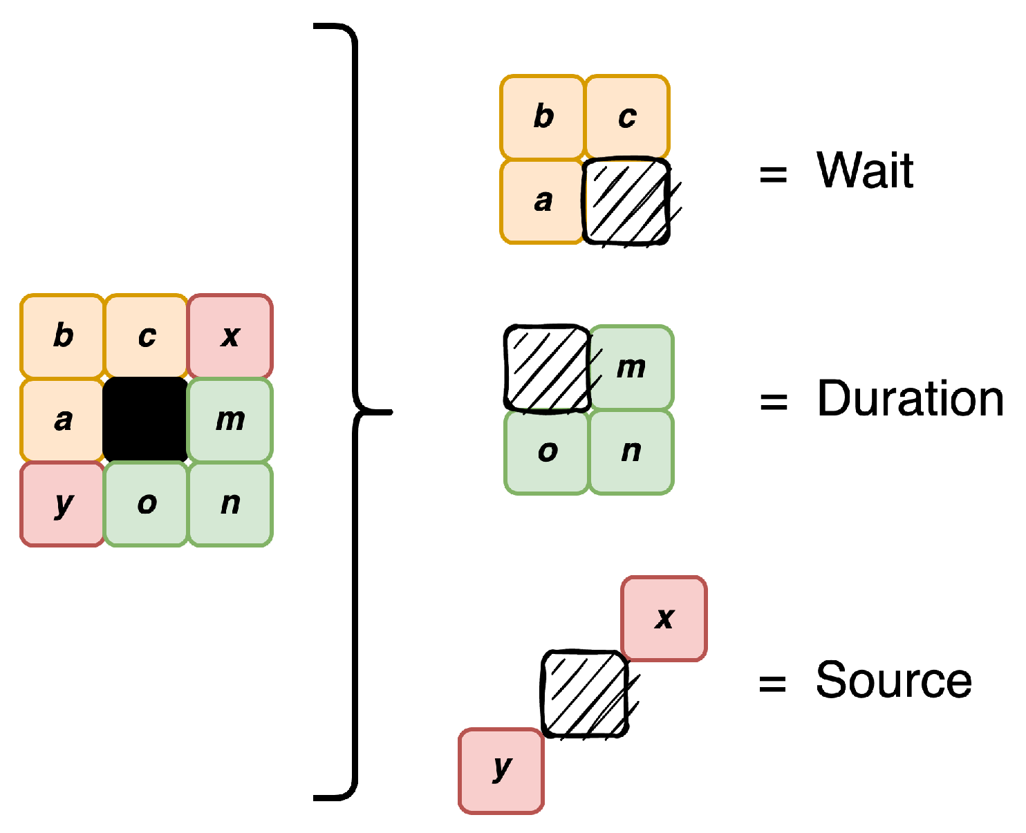
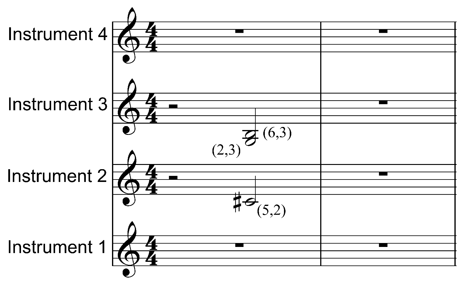
4.2.2. Placing the Pitches in the Frame: Wait and Duration

As mentioned at the beginning of Section 4.2, the 8 × 4 grid in Figure 22 defines a frame for two 4/4 measures of music. We have already established that the cell ( 5 , 2 ) yields the pitch C 4 , which is to be played by the second instrument (counting from the bottom to the top of the score) of an ensemble of four (Figure 27). To calculate the placement of this pitch on the frame, the system builds two codes based on the values of the respective neighbouring cells, as shown in Figure 25: ( a b c ) for waits and ( m n o ) for durations. Thus, Wait ( 5 , 2 ) = 000 and Duration ( 5 , 2 ) = 000 , which retrieves a minim figure (or a half note in North American English). In this case, note C 4 starts after two beats from the beginning and lasts for another two beats. The complete frame with all three notes is shown in Figure 27. In this example, the cells were processed from the bottom to the top and from the left to the right of the grid, in this order: (5,2), (2,3) and (6,3).

5. Real Examples from Qubism

We are now in a position to examine two real examples of generating musical materials for the composition Qubism. The first example used a one-dimensional PQCA to generate a rhythmic sequence of clusters. The second used a two-dimensional PQCA to produce a polyphonic musical sequence.

5.1. Composing Rhythmic Clusters

The first example used the sources of pitches and duration codes shown in Figure 19 and Figure 20, in Section 4.1.
We partitioned the PQCA bar of 18 cells into nine pairs of supercells. Similarly to the instance in Figure 7, we defined two partition schemes. One of which was a shifted version of the other by one cell.
Next, we specified two update frames, one for each of the partitions, and the global update circuit. Figure 28 and Figure 29 show the respective local circuits for the update frames, and the global update circuit is depicted in Figure 30.
As briefly mentioned in Section 2.2, the qubits in a quantum circuit typically start in the ground state | 0 . However, here we wanted to initialise the cells of the PQCA with random values. To this end, we implemented a simple quantum dice [37] to generate truly random values to initialise them. This resulted in the following initial cell values: [1, 1, 1, 0, 1, 1, 1, 0, 0, 1, 1, 0, 0, 0, 0, 1, 0, 0]. Thus, the system needed to adapt the global update circuit before sending it to the backend for processing. When a cell was equal to one, the system added an X gate at the beginning of the circuit to flip the respective qubit to | 1 . Figure 30 shows the circuit for the first cycle. On the left side of the dashed line are the gates to initialise the qubits. Such update must be done for every cycle of the PQCA to set the qubits with the results from the last measurement.
The circuit (Figure 30) required 18 qubits. It was run on ibmq_toronto, which is a 27-qubit superconducting Falcon processor made by IBM Quantum. We ran it for 50 cycles, with 30,000 shots per cycle. Figure 31 shows the resulting rhythmic sequence of clusters and Figure 32 depicts the cellular sequence that produced it.

5.2. Composing Musical Forms

The two-dimensional example used the sources of reference pitches shown in Figure 23 and the codes for waits and duration shown in Figure 24. The transposition coefficients were defined as follows: Δ = [ 7 , 4 , 5 , 0 , 12 , 3 , 2 , 1 ] .
This PQCA used an 8 × 12 cellular grid. Therefore, each cycle produced two 4 4 measures of music for twelve instruments.
We defined two partition schemes, forming 48 supercells each. One scheme partitioned the grid into horizontal pairs and the other into vertical pairs. Then, we defined two update frames, one for each partition. The respective update circuits are shown in Figure 33 and Figure 34.
The global update circuit is shown in Figure 35. As it requires 96 qubits, only a partial view of the circuit is printed. Put simply, in the full version, the shown block of 24 qubits is repeated four times. For this PQCA, the initial values of the entire grid were 0s. It was run on ibm_washington, which is a 127-qubit superconducting Eagle processor made by IBM Quantum. We ran it for 50 cycles of 80,000 shots per cycle. Figure 36 depicts the cellular sequence resulting from the first four cycles of the PQCA and Figure 37 shows the respective resulting musical forms: there are eight measures of music, two measures per cycle.

5.3. Implementation Considerations

The systems were implemented in Python [38] and Qiskit [39], an open-source SDK for programming quantum computers. The ICCMR team developed and maintain a Python package for designing and executing PQCA, which is publicly available. The PQCA package and accompanying tutorials, including music mapping examples, are available through the ICCMR’s GitHub repository [40,41].
Quantum computing hardware is accessed through IBM Cloud [42]. The global update circuits are optimised using optimisation tools available through t∣ket〉, a software platform developed by Quantinuum [43]. The optimisation reduces the number of gates in a quantum circuit and reconfigures it to perform better on specific devices.
The system generates music notation in MusicXML format using Music21, a Python-based toolkit for computer-aided musicology [44].

6. Concluding Discussion

There have been numerous initiatives to use CA to compose music, e.g., [10,21,22,45,46,47,48]. However, to the best of our knowledge, the work presented here, the PQCA package [40] and the composition Qubism are pioneering the use of quantum CA in music. The PQCA package [40] is now publicly available for other musicians wishing to explore the fascinating possibilities offered by quantum CA.
In the introduction, we mentioned that we were interested in developing AI technology to support musicians to create original music, rather than imitations of existing repertoires. Moreover, we emphasised the term “support” because we are not interested in systems that create compositions autonomously.
Music expresses ineffable thoughts, highly personal impressions of the world and emotions. Of course, music is also logical, systematic and follows guiding rules. Rationality does play an important role in music composition, especially classical music. However, music that is generated totally automatically is rather meaningless. Music should be embedded in cultural and emotionally meaningful contexts, which composers express in subtle ways, which are largely beyond description. A computer would not be capable of composing a piece such as Beethoven’s Symphony No. 3 autonomously. Its backstory, myriad references, drama and so on, are aspects of musicianship that computers, as we know them today, cannot grasp.
Obviously, composers ought to explore the technologies of their time. Undoubtedly, the most influential music technology of the 21st century is the computer: a general-purpose device that can be programmed to generate music following logical operations. Moreover, computers facilitate musical composition informed by processes and data abstracted from phenomena other than music. CA models are a case in point.
However, computing technology is constantly evolving, and emerging quantum computers are a nascent technology, which is bound to impact the music industry in the time to come.
Despite the various theoretical demonstrations and proof-of-principles of the advantages that future quantum computers will bring over existing classical ones (e.g., [49,50]), we are not in a position here to advocate any quantum advantage for musical applications. What we advocate, however, is that the music technology community should be quantum-ready for when quantum computing hardware becomes more sophisticated, widely available and possibly advantageous for creativity and business. In the process of learning and experimenting with this new technology, novel approaches, creative ideas and innovative applications are bound to emerge. Nevertheless, we argue that it would be impossible to generate the musical examples shown in this paper without a quantum computer.
The methods described in the paper to map PQCA outputs onto music are, of course, arbitrary. There might be infinite ways of doing this, and it would be untenable to compare those methods objectively. One could ask: Does the music produced with method “a” sound more interesting than the music produced with method “b”? To answer this question, we would need to define “interesting”. This is not trivial. We rather propose that the design of such methods should be considered as part of a compositional process. Different composers or different pieces should explore different methods. In the case of the systems presented here, they were not designed to produce music ready to be played. We intentionally designed them to produce material to be further developed by a human composer. Indeed, the examples in Figure 31 and Figure 37 are sketches for Qubism. Dozens of such sketches were produced. These were the raw materials for the composition. With these materials, the composer (E.R.M.) further developed them into a fully fledged piece.

Author Contributions

Conceptualization, E.R.M.; methodology, E.R.M.; software, H.S.; investigation, E.R.M. and H.S.; resources, E.R.M.; writing—original draft preparation, E.R.M. and H.S.; writing—review and editing, E.R.M.; project administration, E.R.M. All authors have read and agreed to the published version of the manuscript.

Funding

This research received no external funding.

Acknowledgments

This work was developed as part of E.R.M. research residency at the Center for Quantum Technologies and Applications (CQTA) in DESY (Deutsches Elektronen-Synchrotron), Zeuthen, Germany, in 2022. The authors would like to thank CQTA for enabling access to IBM Quantum computer resources. In particular, we are indebted to Karl Jansen and his team, for their support and advice.

Conflicts of Interest

The authors declare no conflict of interest.

References

  1. Miranda, E.R. (Ed.) Handbook of Artificial Intelligence for Music Foundations, Advanced Approaches, and Developments for Creativity; Springer International Publishing: Cham, Switzerland, 2021. [Google Scholar]
  2. Cope, D. Experiments in Musical Intelligence; A-R Editions: Madison, WI, USA, 1996. [Google Scholar]
  3. Woods, W.A. Transition network grammars for natural language analysis. Commun. ACM 1970, 13, 591–606. [Google Scholar] [CrossRef]
  4. Kuang, J.; Yang, T. Popular Song Composition Based on Deep Learning and Neural Networks. J. Math. 2021, 2021, 7164817. [Google Scholar] [CrossRef]
  5. Graupe, D. Deep Learning Neural Networks; World Scientific: Singapore, 2016. [Google Scholar]
  6. Hernandez-Olivan, C.; Beltran, J.R. Music Composition with Deep Learning: A Review. arXiv 2021, arXiv:2108.12290. [Google Scholar]
  7. Romero, J.; Ekart, A.; Martins, T.; Correia, J. (Eds.) Artificial Intelligence in Music, Sound, Art and Design; LNCS 12103; Springer International Publishing: Cham, Switzerland, 2020. [Google Scholar]
  8. Waugh, I. Datamusic Fractal Music. Music. Technol. 1991, October, 62–66. [Google Scholar]
  9. Epstein, J.M.; Axtell, R. The Fractal Geometry of Nature; W. H. Freeman: New York, NY, USA, 1982. [Google Scholar]
  10. Miranda, E.R. Cellular Automata Music: An Interdisciplinary Project. J. New Music. Res. 1993, 22, 3–21, (formerly known as Interface). [Google Scholar] [CrossRef]
  11. Shiff, J.L. Cellular Automata: A Discrete View of the World; Wiley: Hoboken, NJ, USA, 2011. [Google Scholar]
  12. Cao, Y.; Romero, J.; Olson, J.P.; Degroote, M.; Johnson, P.D.; Kieferova, M.; Kivlichan, I.D.; Menke, T.; Peropadre, B.; Sawaya, N.P.D.; et al. Quantum Chemistry in the Age of Quantum Computing. Chem. Rev. 2019, 19, 10856–10915. [Google Scholar] [CrossRef]
  13. Kerenidis, I.; Prakash, A. Quantum recommendation systems. In Proceedings of the 2017 Conference on Innovations in Theoretical Computer Science, Berkeley, CA, USA, 9–11 January 2017. [Google Scholar] [CrossRef]
  14. Oshiro, S. QuiKo: A Quantum Beat Generation Application. In Quantum Computer Music Foundations, Methods and Advanced Concepts; Miranda, E.R., Ed.; Springer: Cham, Switzerland, 2022. [Google Scholar]
  15. Clemente, G.; Crippa, A.; Jansen, K.; Tuysuz, C. New Directions in Quantum Music: Concepts for a Quantum Keyboard and the Sound of the Ising Model. In Quantum Computer Music Foundations, Methods and Advanced Concepts; Miranda, E.R., Ed.; Springer: Cham, Switzerland, 2022. [Google Scholar]
  16. Weaver, J. Quantum Music Playground Tutorial. In Quantum Computer Music Foundations, Methods and Advanced Concepts; Miranda, E.R., Ed.; Springer: Cham, Switzerland, 2022. [Google Scholar]
  17. Arrighi, P.; Grattage, J. Partitioned quantum cellular automata are intrinsically universal. arXiv 2010, arXiv:1010.2335. [Google Scholar] [CrossRef]
  18. Miranda, E.R.; Miller-Bakewell, H. Cellular Automata Music Composition: From Classical to Quantum. In Quantum Computer Music Foundations, Methods and Advanced Concepts; Miranda, E.R., Ed.; Springer: Cham, Switzerland, 2022. [Google Scholar]
  19. Clark, S.; Rehding, A. Music in Time: Phenomenology, Perception, Performance; Harvard University Press: Cambridge, MA, USA, 2016. [Google Scholar]
  20. Dustan, R. The Composer’s Handbook: A Guide to the Principles of Musical Composition; Leopold Classic Library: South Yarra, VIC, Australia, 2017. [Google Scholar]
  21. Beyls, P. The musical universe of cellular automata. In Proceedings of the International Computer Music Conference (ICMC), Columbus, OH, USA, 2–5 November 1989; pp. 34–41. [Google Scholar]
  22. Hoffmann, P. Towards an automated art: Algorithmic processes in Xenakis’ compositions. Contemp. Music. Rev. 2002, 21, 121–131. [Google Scholar] [CrossRef]
  23. Miranda, E.R. Cellular automata music: From sound synthesis to musical forms. In Evolutionary Computer Music; Miranda, E.R., Biles, J.A., Eds.; Springer: London, UK, 2007. [Google Scholar]
  24. Love, P.; Boghosian, B. From Dirac to Diffusion: Decoherence in Quantum Lattice Gases. Quantum Inf. Process. 2005, 4, 335–354. [Google Scholar] [CrossRef]
  25. Preston, K.; McDuff, M.J.B. Modern Cellular Automata: Theory and Applications; Springer International Publishing: Cham, Switzerland, 1984. [Google Scholar]
  26. Hogeweg, P. Cellular automata as a paradigm for ecological modeling. Appl. Math. Comput. 1988, 27, 81–100. [Google Scholar] [CrossRef]
  27. Ermentrout, G.B.; Edelstein-Keshet, L. Cellular automata approaches to biological modeling. J. Theor. Biol. 1993, 160, 97–133. [Google Scholar] [CrossRef]
  28. Epstein, J.M.; Axtell, R. Growing Artificial Societies: Social Sciences from the Bottom Up; The MIT Press: Cambridge, MA, USA, 1996. [Google Scholar]
  29. Miranda, E.R. Generating Source Streams for Extralinguistic Utterances. J. Audio Eng. Soc. 2002, 50, 165–172. [Google Scholar]
  30. Burks, A.W. (Ed.) Essays on Cellular Automata; University of Illinois Press: Champaign, IL, USA, 1971. [Google Scholar]
  31. Gardner, M. The fantastic combinations of John Conway’s new solitaire game “life”. Sci. Am. 1970, 223, 120–123. [Google Scholar] [CrossRef]
  32. Nielsen, M.A.; Chuang, I.L. Quantum Computation and Quantum Information, 10th Anniversary Edition; Cambridge University Press: New York, NY, USA, 2011. [Google Scholar]
  33. Ekert, A.; Macchiavello, C. An Overview of Quantum Computing. In Unconventional Models of Computation; Calude, C.S., Casti, J., Dinneen, M.J., Eds.; Springer: Singapore, 1997. [Google Scholar]
  34. Sutor, R.S. Dancing with Qubits: How Quantum Computing Works and How It Can Change the Word; Packt: Birmingham, UK, 2019. [Google Scholar]
  35. Farrelly, T. A review of quantum cellular automata. Quantum 2020, 4, 368. [Google Scholar] [CrossRef]
  36. Inokuchi, S.; Mizoguchi, Y. Generalized partitioned quantum cellular automata and quantization of classical CA. arXiv 2003, arXiv:quant-ph/0312102. [Google Scholar]
  37. Miranda, E.R. Creative Quantum Computing: Inverse FFT Sound Synthesis, Adaptive Sequencing and Musical Composition. In Handbook of Unconventional Computing; Adamatzky, A., Ed.; World Scientific: Singapore, 2021. [Google Scholar]
  38. Python Programming Language Documentation. Available online: https://www.python.org/ (accessed on 27 December 2022).
  39. Qiskit Documentation. Available online: https://qiskit.org/ (accessed on 27 December 2022).
  40. PQCA Repository. Available online: https://github.com/iccmr-quantum/pqca (accessed on 27 December 2022).
  41. PQCA Tutorial. Available online: https://github.com/iccmr-quantum/PQCA_Tutorial (accessed on 27 December 2022).
  42. IBM Quantum Computer Resources. Available online: https://www.ibm.com/quantum (accessed on 27 December 2022).
  43. Sivarajah, S.; Dilkes, S.; Cowtan, A.; Simmons, W.; Edgington, A.; Duncan, R. t|ket〉: A retargetable compiler for NISQ devices. Quantum Sci. Technol. 2020, 6, 014003. [Google Scholar] [CrossRef]
  44. Music 21 Documentation. Available online: https://web.mit.edu/music21/ (accessed on 27 December 2022).
  45. Bilotta, E.; Pantano, P.; Talarico, V. Music Generation through Cellular Automata: How to Give Life to Strange Creatures. Research Gate. Available online: https://www.researchgate.net/publication/2324938_Music_Generation_through_Cellular_Automata_How_to_Give_Life_to_Strange_Creatures (accessed on 28 December 2022).
  46. Burraston, D.M. Generative Music and Cellular Automata. Ph.D. Thesis, University of Technology, Sydney, Australia, 2006. Available online: https://www.noyzelab.com/uploads/1/2/6/1/126197943/dburraston-genmusic_ca-phd-thesis.pdf (accessed on 28 December 2022).
  47. Delarosa, O.; Soros, L.B. Growing MIDI Music Files Using Convolutional Cellular Automata. In Proceedings of the IEEE Symposium Series on Computational Intelligence (SSCI), Canberra, ACT, Australia, 1–4 December 2020. [Google Scholar] [CrossRef]
  48. Nedjah, N.; Bezerra, H.D.; Mourelle, L.M. Automatic generation of harmonious music using cellular automata based hardware design. Integration 2018, 61, 205–223. [Google Scholar] [CrossRef]
  49. Gibney, E. Hello quantum world! Google publishes landmark quantum supremacy claim. Nature 2019, 574, 461–463. [Google Scholar] [CrossRef]
  50. Huang, H.-Y.; Broughton, M.; Cotler, J.; Chen, S.; Mohseni, M.; Neven, H.; Babbush, R.; Kueng, R.; Preskill, J.; McClean, J.R. Quantum advantage in learning from experiments. Science 2022, 367, 1182–1186. [Google Scholar] [CrossRef] [PubMed]
Figure 1. An example of a one-dimensional CA consisting of a bar of 13 cells.
Applsci 13 02401 g001
Figure 2. An example of a two-dimensional CA consisting of a grid of 36 cells.
Applsci 13 02401 g002
Figure 3. A Bloch sphere representing a single qubit. Source: Smite-Meister, https://commons.wikimedia.org/w/index.php?curid=5829358 (accessed on 2 January 2023).
Applsci 13 02401 g003
Figure 4. Circuit representation of the CX gate. In this case, q 1 will be flipped only if q 0 is | 1 .
Applsci 13 02401 g004
Figure 5. An example of a quantum circuit showing a sequence of quantum gates, the first of which are two H gates applied to q 3 and q 4 , followed by a CX gate with q 4 as a control to flip the state of q 0 and so on.
Applsci 13 02401 g005
Figure 6. A bar of twelve cells.
Applsci 13 02401 g006
Figure 7. At the top is a bar of twelve cells partitioned into six supercells, two cells long each. At the bottom is a shifted version of the partition.
Applsci 13 02401 g007
Figure 8. A simple local updating circuit for a supercell comprising two qubits.
Applsci 13 02401 g008
Figure 9. An example of a global quantum circuit for a one-dimensional PQCA.
Applsci 13 02401 g009
Figure 10. An example of five cycles of a one-dimensional PQCA. (Note: the colours of the squares stand for the measured values of the automaton. A black cell represents the number 1 and a white one the number 0.)
Applsci 13 02401 g010
Figure 11. A grid of 4 × 4 cells for a two-dimensional PQCA.
Applsci 13 02401 g011
Figure 12. A grid of 4 × 4 cells partitioned into horizontal pairs of cells.
Applsci 13 02401 g012
Figure 13. A grid of 4 × 4 cells partitioned into vertical strips of four cells each.
Applsci 13 02401 g013
Figure 14. Local update circuit made of two qubits.
Applsci 13 02401 g014
Figure 15. Local update circuit made of four qubits.
Applsci 13 02401 g015
Figure 16. An example of a global update circuit for a two-dimensional PQCA.
Applsci 13 02401 g016
Figure 17. A pattern produced with nine cycles of the global update circuit shown in Figure 16. All cells started with | 0 .
Applsci 13 02401 g017
Figure 18. Coding scheme for representing a cluster of musical notes.
Applsci 13 02401 g018
Figure 19. A set of four sources of pitches to build clusters.
Applsci 13 02401 g019
Figure 20. One-dimensional PQCA codes for note durations.
Applsci 13 02401 g020
Figure 21. An example of a cluster generated with A = { 11 } and D = { 011001001001 } .
Applsci 13 02401 g021
Figure 22. A 8 × 4 grid of cells. Three cells are equal to 1.
Applsci 13 02401 g022
Figure 23. Sources of reference pitches for two-dimensional PQCA.
Applsci 13 02401 g023
Figure 24. Two-dimensional PQCA codes for waits and durations.
Applsci 13 02401 g024
Figure 25. Coding scheme for the two-dimensional PQCA.
Applsci 13 02401 g025
Figure 26. Adding four semitones to pitch A 3 results in C 4 .
Applsci 13 02401 g026
Figure 27. The musical rendering of the PQCA in Figure 22.
Applsci 13 02401 g027
Figure 28. The local circuit for the first update frame of the one-dimensional PQCA example.
Applsci 13 02401 g028
Figure 29. The local circuit for the second update frame of the one-dimensional PQCA example.
Applsci 13 02401 g029
Figure 30. Global update circuit for the one-dimensional PQCA example. On the left side of the red dashed line are the gates to initialise the qubits.
Applsci 13 02401 g030
Figure 31. The resulting rhythmic sequence of clusters.
Applsci 13 02401 g031
Figure 32. The resulting cellular sequence.
Applsci 13 02401 g032
Figure 33. A local updating circuit for the first update frame of the two-dimensional example.
Applsci 13 02401 g033
Figure 34. A local updating circuit for the second update frame of the two-dimensional example.
Applsci 13 02401 g034
Figure 35. The global update circuit for the polyphonic musical example.
Applsci 13 02401 g035
Figure 36. Cellular sequence resulting from the first four cycles of the PQCA.
Applsci 13 02401 g036
Figure 37. Resulting musical form for twelve instruments.
Applsci 13 02401 g037
Disclaimer/Publisher’s Note: The statements, opinions and data contained in all publications are solely those of the individual author(s) and contributor(s) and not of MDPI and/or the editor(s). MDPI and/or the editor(s) disclaim responsibility for any injury to people or property resulting from any ideas, methods, instructions or products referred to in the content.

