Low Complexity Deep Learning Framework for Greek Orthodox Church Hymns Classification

Abstract

The Byzantine religious tradition includes Greek Orthodox Church hymns, which significantly differ from other cultures’ religious music. Since the deep learning revolution, audio and music signal processing are often approached as computer vision problems. This work trains from scratch three different novel convolutional neural networks on a hymns dataset to perform hymns classification for mobile applications. The audio data are first transformed into Mel-spectrograms and then fed as input to the model. To study in more detail our models’ performance, two state-of-the-art (SOTA) deep learning models were trained on the same dataset. Our approach outperforms the SOTA models both in terms of accuracy and their characteristics. Additional statistical analysis was conducted to validate the results obtained.

1. Introduction

The heritage sectors of culture and religion require the extensive study of diverse data, which has led to the consideration of machine learning (ML) and deep learning (DL) methodologies as complementary to traditional signal processing techniques [1]. Recently, the great success of DL approaches in several computer vision (CV) problems has led to their application in audio signal processing problems too. More specifically, the audio data are usually transformed into spectrograms (images) and then CV methods are employed [2].

Convolutional neural networks (CNNs) have been trained to extract useful information from images such as paintings’ styles [3], music features [4], and optical music classification [5]. CNNs’ success in image classification is attributed to their ability to apply filters for feature extraction and exploit images’ grid topology [6]. As a result, such models are often trained on audio and music signal processing problems [7].

However, ML and DL techniques face many challenges when they are designed for mobile applications [8,9,10]. DL models require extensive computational power for their training, and even after training, their weights occupy large portions of memory. To overcome such challenges, DL approaches for mobile devices are designed to be lightweight and are often trained either offline or in the cloud.

Audio signal processing applications, such as voice recognition, music genre classification, sound identification, and cultural heritage music classification, form many of today’s mobile applications that utilize ML/DL methodologies. Recognizing and classifying Greek Orthodox Church hymns is a challenging task due to their vocal nature, lack of musical accompaniment, and differing climaxes from Western hymns. Furthermore, the Byzantine chants are monodic, in free rhythm, and often try to illustrate the meaning of the words melodically. The language used is Greek, while the measure of the music is often altered to serve the poetic text so that it can be properly emphasized. Finally, the way the verse is pronounced in particular ways, to precisely support the poetic text. Breathing in the middle of a word or within a single meaning (e.g., between adjective and noun) is forbidden. Usually, breaths are only in commas and dots in the text. Such characteristics are also met in other Eastern Orthodox Church hymns, such as the Russian Church, the Ukrainian Church, the Serbian Church, etc. The authors have collected a corpus of 23 Greek Orthodox Church hymns with 4820 performances in total. The audio samples are first transformed into Mel-spectrograms, and then three different novel CNN architectures are trained in a supervised learning framework for the task of Greek Orthodox Church hymns identification, while five pre-trained DL models are tested on the same problem.

The main contributions of this research may be summarized as follows:

• Three novel DL models based on convolution operation are designed for Greek Orthodox Church hymns classification. A novel Visual Geometry Group (VGG) approach is presented, namely Micro VGG, which is custom-made for this problem and outperforms the other custom architectures. Micro VGG is lightweight and its fast convergence makes it suitable for mobile applications.
• Five state-of-the-art (SOTA) models are tested on the problem of Greek Orthodox Church hymns classification. A comparison study between the different DL approaches is conducted, both in terms of prediction accuracy and in terms of computational cost.

Our approach differs from conventional applications like Shazam in several ways. First, Shazam identifies songs based on an audio fingerprint which is related to the acquired spectrogram. Shazam identifies specific points in the spectrogram that correspond to peaks indicating higher energy content. By focusing on these peak points, the algorithm effectively minimizes the impact of background noise during audio identification. Shazam constructs its fingerprint catalog using a hash table, wherein the frequency serves as the key. Instead of marking only a single point in the spectrogram, Shazam marks a pair of points: the peak intensity along with a secondary anchor point. As a result, its database key comprises a hash of the frequencies of both points, rather than a single frequency. This approach reduces the occurrence of hash collisions, thereby enhancing the performance of the hash table [11]. However, one of the main drawbacks of Shazam is the fact that it is very sensitive to which version of a track has been sampled, making the maximum number of false predictions a parameter that needs to be tuned depending on the application [12]. On the contrary, our method is based on knowledge retrieval. A DL model learns the features that characterize each data sample. The proposed DL approaches are designed to be applied to any audio dataset that contains music without instruments. Micro VGG can be trained on small datasets to perform audio classification. Its architecture is based on the classical VGG model. Thus, it can exploit its non-linear behavior to extract valuable features from the acquired spectrograms. To the best of the authors’ knowledge, it is the first time that the Greek Orthodox Church hymns classification problem is addressed using a DL framework.

1.1. Related Work

DL has found several applications in audio and music signal processing [13]. Although DL has advanced audio technology, leading to commercial applications such as music recommendation systems [14], its main success lies in music information retrieval (MIR) and music generation (MG). MIR may be defined as the set of techniques that are used to extract valuable information from audio data [2], while MG is formed by methods that generate new audio content [15]. Music data classification and identification are formulated as MIR problems; hence, our literature review will focus on this field.

Several different CNN models have been utilized for music identification and audio classification. The authors in [16] train a CNN model and a tensor deep stacking network for sound classification. The CNN is trained on two datasets with environmental sound data samples. The DL architecture is structured with two convolution layers and one fully connected. Finally, the tensor deep stacking network is trained using two stacked blocks, then with three stacked blocks, and finally with four stacked blocks. The work presented in [7] employs an ensemble of learners for audio classification. More specifically, five pre-trained CNN models, namely AlexNet [17], GoogleNet [18], VGGNet [19], ResNet [20], and InceptionV3 [21], form an ensemble classifier that achieves better performance overall. Two of the most successful CNNs for audio identification tasks are the VGGish and the YAMNet models [22]. VGGish is a pre-trained CNN that is inspired by the VGG networks. The model consists of a series of convolution and activation layers, optionally followed by a max pooling layer. This network contains 17 layers in total. These two models, together with GoogleNet, SqueezeNet [23], and ShuffleNet [24] are tested in a comparative study that is provided in [25]. VGGish achieves the best classification accuracy.

DL relies heavily on large amounts of data; hence, publicly available datasets are considered valuable. AudioSet [26] is an audio-event dataset widely used in audio classification problems. More specifically, DL models are often pre-trained on AudioSet before their application in a different problem, exploiting the transfer learning capabilities.

Audio ML/DL on mobile devices has recently emerged as a new research area. In [27], ML algorithms are used for monitoring environmental sounds. The authors seek to find whether it is feasible to create a measurement system for environmental sound monitoring that runs on a handheld device and uses ML to provide meaningful readings. The authors in [28] perform audio-visual speech and gesture recognition using CNN architectures that combine convolution and recurrent operations. A novel DL-based speech enhancement method for dual microphone cell phones is presented in [29] utilizing a CNN with a recurrent architecture. The proposed densely connected convolutional recurrent network employs an encoder-decoder scheme to achieve both a good feature extraction and sequential modeling of the available audio data.

Recently, DL has been employed for music genre recognition problems. A novel CNN model for Persian music genre recognition, namely PMG-Net, is introduced in [30]. The authors created and made publicly available the PMG-Data dataset, which consists of 500 music samples from different genres of Pop, Rap, Traditional, Rock, and Monody. Furthermore, after the data pre-processing, the desired features are fed to PMG-Net. PMG-Net is based on the VGG-16 architecture; however, it only consists of two equal-size filters in two subsequent layers. The work presented in [31] provides a novel feature extraction algorithm, also utilizing the tunable Q-wavelet transform. The extracted features are fed into several ML classifiers.

1.2. Organization of the Article

The rest of this work is structured as follows: In Section 2, the data pre-processing methods are presented along with the CNN architectures, while in Section 3 the experiments and the results are discussed. Section 4 is devoted to the discussion of the results. Section 5 concludes this work by highlighting the most important remarks.

Notation and abbreviations: In this work, we use lowercase Latin letters for scalars, matrices are denoted with capital bold letters, i.e., $\mathbf{W}$, and vectors with lowercase bold letters, i.e., $\mathbf{x}$. The calligraphic capital letter is reserved for the mathematical operators, i.e., $\mathcal{P}$.

2. Materials and Methods

This section discusses the data generation and processing procedures. Image processing is required for the images to be in a suitable form for the neural networks’ training. In addition, the different CNNs that are designed for the task of Greek Orthodox Church hymns identification are presented in detail.

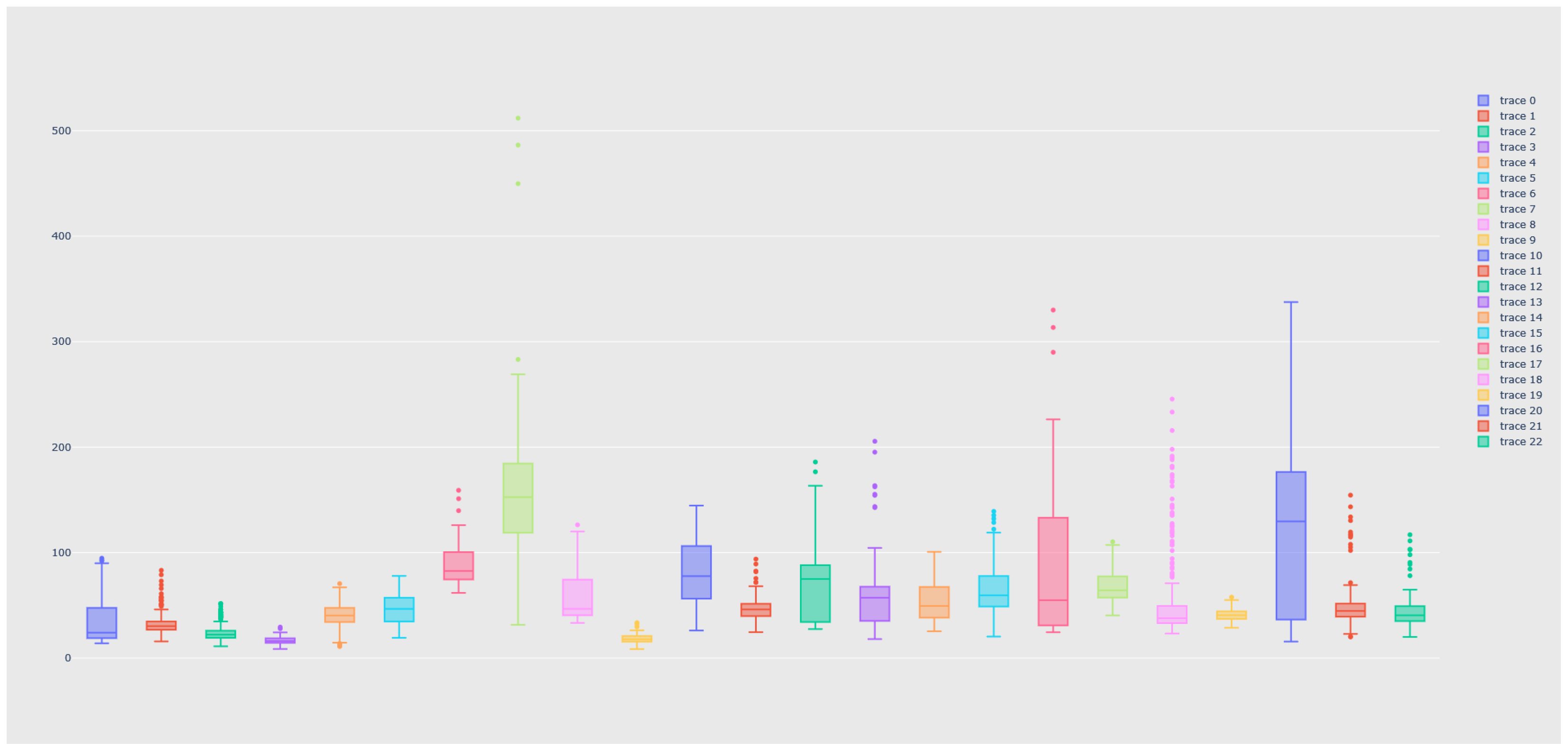
2.1. Data Generation

For this work, the dataset is composed of 23 distinct classes (hymns). The number of samples per class is shown in

Table 1. Number of performances per class.

Class	Samples	Hymn Name (In the Greek Language)
Hymn1	210	H ΠAΡΘΕΝOΣ ΣHΜΕΡOΝ
Hymn2	210	ΕΥΛOΓHΤOΣ ΕΙ ΧΡΙΣΤΕ O ΘΕOΣ
Hymn3	218	ΤHΝ ΩΡAΙOΤHΤA
Hymn4	174	ΤOΝ ΣΤAΥΡOΝ ΣOΥ ΠΡOΣΚΥΝOΥΜΕ
Hymn5	210	AΝOΙΞΩ ΤO ΣΤOΜA ΜOΥ
Hymn6	210	ΦΩΣ ΙΛAΡOΝ
Hymn7	210	ΜΕΤA ΤΩΝ AΓΙΩΝ AΝAΠAΥΣOΝ
Hymn8	210	ΧΡΙΣΤOΣ AΝΕΣΤH
Hymn9	210	ΜΕΤA ΠΝΕΥΜAΤΩΝ ΔΙΚAΙΩΝ
Hymn10	222	ΕΙΣ ΤHΝ ΚAΤAΠAΥΣΙΝ ΣOΥ ΚΥΡΙΕ
Hymn11	210	ΠΡOΣΤAΣΙA ΤΩΝ ΧΡΙΣΤΙAΝΩΝ
Hymn12	210	ΔOΞOΛOΓΙA
Hymn13	210	AΝAΣΤAΣΕΩΣ HΜΕΡA
Hymn14	210	ΤOΝ ΝΥΜΦΩΝA ΣOΥ ΒΛΕΠΩ
Hymn15	210	ΤOΥ ΔΕΙΠΝOΥ ΣOΥ ΤOΥ ΜΥΣΤΙΚOΥ
Hymn16	210	AΠOΣΤOΛOΙ ΕΚ ΠΕΡAΤΩΝ
Hymn17	210	ΘΕOΣ ΚΥΡΙOΣ
Hymn18	216	ΘΕOΤOΚΕ ΠAΡΘΕΝΕ
Hymn19	213	ΠAΣA ΠΝOH
Hymn20	207	ΩΣ ΤΩΝ AΙΧΜAΛΩΤΩΝ
Hymn21	210	ΜΕΓAΝ ΕΥΡAΤO
Hymn22	210	ΕΚ ΝΕOΤHΤOΣ ΜOΥ
Hymn23	210	ΜΕΤA ΠΝΕΥΜAΤΩΝ ΔΙΚAΙΩΝ

. Every sample corresponds to a unique interpretation of a Greek Orthodox Church hymn. To enhance the dataset’s diversity, some of the hymns were recorded in a soundproof environment by a single chanter using professional recording equipment, while others were captured using a mobile phone in various churches during divine services, including background noise from crowds and church bells. During the recordings inside the churches, the mobile phone was placed in different places each time to achieve diversity in the audio quality. This strategy was implemented to aid the CNN model in learning distinct features, allowing it to recognize Greek Orthodox Church hymns recorded in any location. The data samples recorded in situ form 50% of the whole dataset. The equal split between the hymns recorded in a soundproof environment and those that were captured during the divine service aims to mitigate the bias from the dataset.

Regarding the statistical properties of our dataset, the minimum duration of a hymn is 20.4 s, while the maximum duration is 117 s. The average duration is 52.8 s and the standard deviation is 17.9 s. For each separate class, these values are depicted in the Boxplots in Figure 1.

2.2. Data Processing

To exploit the SOTA CV techniques, audio data should be transformed into images through a suitable representation. Here, the image processing techniques that were employed are thoroughly discussed.

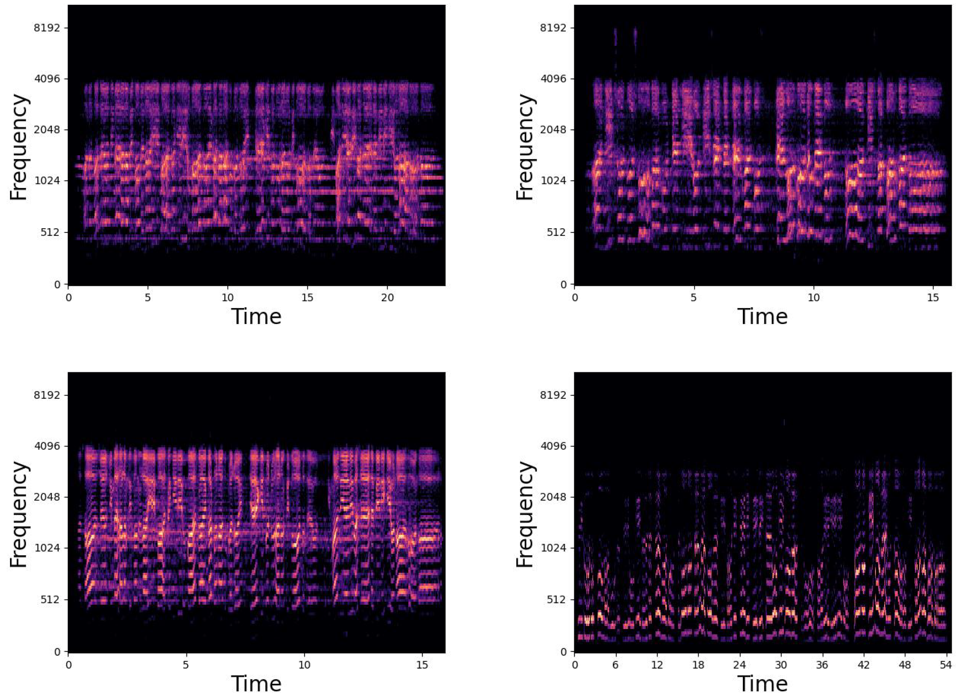
2.2.1. Mel-Spectrograms

To implement CV methodologies, each audio file is converted into a spectrogram. Since the audio files feature human voices, Mel-spectrograms are utilized. A spectrogram can be described as the result of the fast Fourier transform (FFT), an algorithm that computes the discrete Fourier transform (DFT), applied on overlapping windowed segments of the audio signal. It also highlights the passage from the time domain representation to the frequency domain representation.

However, humans do not perceive sound on a linear scale. The Mel scale is preferred because it closely approximates human perception and accurately represents the frequencies that humans typically hear. It is an alternative scale of pitches resulting from human listeners’ judgment that a pair of pitches are equally distant. A reference point is established between the two scales by setting a perceptual pitch of 1000 Hz on the regular frequency scale equal to 1000 Mels. Mel spectrograms can be obtained by transforming the regular spectrograms into the Mel scale using the following formula:

$$m=2595log\left(1+\frac{\nu }{700}\right).$$

(1)

$\nu$ denotes the frequency measured in Hertz.

For our purposes, the whole audio file is transformed into Mel-spectrogram. In Figure 2, different examples of Mel spectrograms from our dataset are depicted. The transformation of the audio samples to Mel-spectrograms is performed using a sample rate equal to 22,050, 512 samples between successive frames (hop length) and a 2048 FFT in window length.

For the acquired spectrograms, the mean value of each RGB channel is {0.4680, 0.4225, 0.4795} and the standard deviation is equal to {0.4449, 0.4624, 0.4298}.

2.2.2. Data Processing and Augmentation

The initial dataset consists of 23 classes and 4820 performances. Various data processing augmentation techniques were employed to increase the number of inputs for the DL models. More specifically, the images are resized in a $64\times 64$ format for computational cost reduction purposes, while the pixel values are normalized.

There are many data augmentation techniques for CV problems, such as random cropping, image rotation, image blurring with a Gaussian filter, etc. A recently introduced data augmentation method is the TriviaAugment (TA) algorithm [32]. TA works as follows. Let $\mathcal{X}$ be an image from our dataset and $\mathcal{T}$ be a set of augmentations. An augmentation is mathematically defined as a function

$$f:\mathcal{D}\times {\mathbb{Z}}^{+}\to \mathcal{A}$$

(2)

Here, $\mathcal{D}$ refers to the image dataset, $\mathcal{A}$ represents the set of the augmented images and a discrete strength parameter is defined in ${\mathbb{Z}}^{+}$.

TA takes as input an image $\mathcal{X}$ and the set $\mathcal{T}$. In the next step, TA samples uniformly at random an augmentation mapping from $\mathcal{T}$ and applies it to the given image $\mathcal{X}$, assigning a strength value s and returns the augmented image. The whole procedure is depicted in Algorithm 1.

Algorithm 1 TA algorithm

Dataset $\mathcal{D}$ with M images     while $m\le M$  do          Pick an image $\mathcal{X}\in \mathcal{D}$          Sample augmentation f from $\mathcal{T}$          Sample a strength value s          Return $f(\mathcal{X},s)$     end while

Another popular data augmentation technique that is employed in our work is the MixUp augmentation [33]. Given two images from the available data selected randomly, MixUp generates a weighted combination of them. Mathematically, this process is formulated as follows: If $({\mathbf{x}}_1,y_1)$ and $({\mathbf{x}}_2,y_2)$ is the chosen image pair, the synthetic image is generated as

$$\begin{array}{cc}\hfill & \widehat{\mathbf{x}}=w{\mathbf{x}}_1+(1-w){\mathbf{x}}_2\hfill \\ \hfill & \widehat{y}=w{y}_1+(1-w)y_2\hfill \end{array}$$

(3)

The weight coefficient $w\sim$Beta(a = 0.2) is independently sampled.

Finally, a third data augmentation method, namely SpecAugment [34] is utilized. SpecAugment consists of three augmentation policies:

• Time warping: From a uniform distribution with range $[-D,D]$, a starting point $d_0$ and a displacement coefficient d are sampled. A linear warping function $\mathcal{D}\left(t\right)$ is defined, such that the point $d_0$ is mapped to the point $d_0+d$. Time warping is defined in such a way that the warped features at time t are related to the original features by the following equation:

  $${\mathbf{x}}_{warp}\left(\mathcal{D}\left(t\right)\right)={\mathbf{x}}_{orig}$$

  (4)
• Frequency masking: Given a uniform distribution with a range from 0 to $\mathcal{F}$, a mask of size f is randomly chosen. Then, a value $f_0$ is chosen from the interval $[0,f_0-f]$ and the consecutive log-Mel frequency channels $[f_0,f_0+f)$ are masked.
• Time masking: Given a uniform distribution with a range from 0 to $\mathcal{T}$, a mask size $\tau$ is randomly chosen. Then, a value ${\tau }_0$ is chosen from the interval $[0,{\tau }_0-\tau ]$ and the consecutive time steps $[{\tau }_0,{\tau }_0+\tau )$ are masked.

The SpecAugment policy consists of applying these three augmentation methods a fixed number of times [34].

After applying these three data augmentation techniques to our dataset, the number of samples increased to 19,280 images.

2.3. CNN Architectures

CNNs have achieved impressive results in many research areas, including CV, natural language processing (NLP), audio signal processing, and object detection [35]. The building blocks of CNN architectures are the following:

• Input layer: This layer accepts the input data in a form suitable for further processing. Usually, the image data are transformed into multi-dimensional arrays with three color channels.
• Convolution layer: Convolution layers are the building blocks of any CNN architecture. They perform the process of feature extraction. The main difference with a fully connected layer is that convolutional layers are characterized by the neuron’s receptive field. This receptive field indicates that every single unit receives input from only a restricted area of the previous layer.
• Activation function: In the academic literature, the majority of the CNN architectures use as an activation function; either a rectified linear unit (ReLU) function or some kind of a variant. ReLU is mathematically defined as in [6]

  $$\begin{array}{c}\hfill g\left(v\right)=max(0,v).\end{array}$$

  (5)
• Pooling layer: Their purpose is to reduce the size of the incoming data in a computationally efficient manner.
• Flattening: This layer transforms the data into a 1D vector.
• Output layer: This layer outputs the model’s prediction.

Many CNNs utilize several techniques to improve their performance. Dropout [36] was introduced as a regularization technique. When Dropout is utilized, some layer outputs are ignored (“dropped out”) in a random way, which results in a different layer behavior. The main consequence of this method is that, in each step during training, a different “view” of the configured layer takes place. In addition, the training process becomes noisy, since individual nodes within a layer are forced to take on more or less responsibility for the inputs.

Batch normalization [37] is another widely used method for accelerating and stabilizing neural networks’ training. Batch normalization usually calculates during training the mean and standard deviation of each input variable to a layer per mini-batch and uses these results to perform layer standardization. There is an ongoing discussion between ML researchers about the way that batch normalization affects training, particularly if it reduces internal covariance shift or smooths the objective function [38,39].

Weights Initialization

Weights initialization refers to the process of assigning values to the neural network’s weights, thus defining a starting point. However, many works employed random initialization, resulting in many problems such as vanishing or exploding gradients [40]. Other initialization techniques include normal initialization, zero initialization, and random uniform initialization. However, all of these methods are not capable to overcome the aforementioned challenges.

Xavier initialization was introduced in [40] as a way to overcome the aforementioned challenges. Xavier initialization does not focus on the randomization technique but on the number of outputs in the following layer. The weights are initialized from a bounded uniform distribution, such that

$$W\sim U\left[-\frac{\sqrt{6}}{m_j+m_{j+1}},\frac{\sqrt{6}}{m_j+m_{j+1}}\right]$$

(6)

$m_j$ represents the number of incoming network connections and $m_{j+1}$ refers to the number of outgoing network connections.

Xavier initialization mitigates the possibilities for exploding or vanishing gradients since the weights are set neither too close to zero nor too close to 1. In this way, the gradients do not vanish or explode too rapidly. In this paper, all the trained models utilize Xavier initialization.

2.4. Performance Metrics

ML and DL algorithms are evaluated in terms of their performance and their generalization capabilities, using several different performance and statistical metrics. In a supervised learning framework, the most common performance metrics for multi-class classification are presented below [41,42,43]:

• Accuracy is defined as the fraction of correct predictions. It is expressed mathematically as

  $$\mathrm{Accuracy}=\frac{1}{M}\sum _{m=0}^{M-1}\mathcal{I}({\widehat{q}}_n=q_n)$$

  (7)
  M is the number of test classes, ${\widehat{q}}_n$ denotes the ML model class predicted label, $q_n$ is the true class label, and $\mathcal{I}\left(x\right)$ represents the indicator function.
• Precision expresses the ratio of correctly predicted positive classes to all predicted positive classes and in multi-class classification problems is defined as

  $$\mathrm{Precision}=\frac{{\sum }_{l=1}^{L}T{P}_l}{{\sum }_{l=1}^L(T{P}_l+F{P}_l)}$$

  (8)
  L refers to the number of classes, $T{P}_l$ is the number of true positive outcomes, and $F{P}_l$ is the number of false positive outcomes for class label l.
• Recall expresses the ratio of correctly predicted positive classes to all existing positive classes. In mathematical terms,

  $$\mathrm{Recall}=\frac{{\sum }_{l=1}^{L}T{P}_l}{{\sum }_{l=1}^L(T{P}_l+F{N}_l)}$$

  (9)
  L is the number of classes, $T{P}_l$ is the number of true positive, and $F{N}_l$ is the number of false negative for class label l, respectively.
• F₁-score aggregates Precision and Recall metrics under the concept of harmonic mean. This is defined as

  $$F_1-\mathrm{score}=2\times \frac{\mathrm{Precision}\times \mathrm{Recall}}{\mathrm{Precision}+\mathrm{Recall}}.$$

  (10)
  $F_1$-score can be viewed also as the weighted average between Precision and Recall.

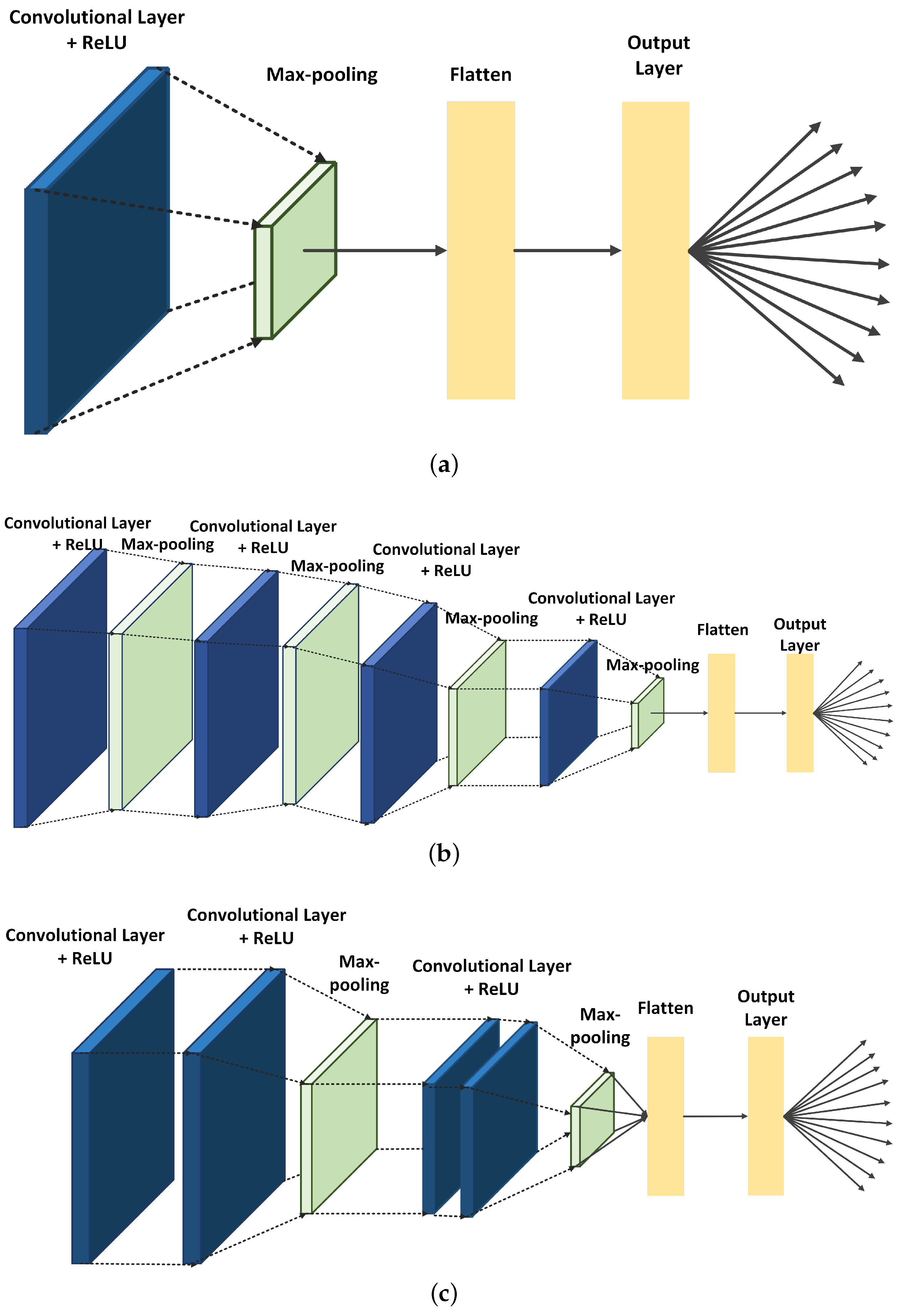
2.5. Proposed Approaches

In this research work, Greek Orthodox Church hymns identification is tackled as a CV problem. To find an optimal solution to this problem, three different CNNs are designed. In Figure 3, the different architectures are depicted.

Initially, a shallow CNN with only one convolution layer is designed; however, it severely underperforms. The next design is a CNN architecture with four convolution layers, dropout and batch normalization, and two fully-connected layers. Although it performs well in terms of accuracy, it requires a significant amount of computational resources. The third solution is a VGG-variant, namely Micro VGG, that outperforms the other two models and is lightweight.

2.5.1. Shallow CNN

As a first approach, a shallow CNN with only one convolution layer followed by a max-pooling layer and two fully-connected layers is designed. The convolution layer has 64 neurons, while the first fully connected has 128 neurons. After several experiments, the best-performing instance of the model utilized the ReLU function. Dropout was used as a mechanism to avoid overfitting. The neurons’ weights were initialized using the Xavier technique.

2.5.2. Deep CNN

The second DL model that was trained to identify Greek Orthodox Church hymnsis a custom CNN with four convolution layers, four max-pooling layers, and two fully-connected layers. The first convolution layer has 64 neurons, and the following layers have 128, 256, and 512 neurons, respectively. Again, the ReLU activation gave the best performance along with dropout and batch normalization, while Xavier initialization was also employed.

2.5.3. Micro VGG

The third model is a variant of VGG architecture. The VGG model was introduced in ImageNet Large Scale Visual Recognition Challenge (ILSVRC) in 2014 [19,44] and since then it has become one of the most successful DL models in CV. The first VGG consists of 16 layers [19]; however, this number is considered too big for a small dataset, since it would allow the model to overfit rapidly. In our case, the Micro VGG consists only of two blocks of convolution layers, with 64 neurons each and $3\times 3$ kernel. Xavier initialization is also employed. Batch normalization is again employed. The last two layers are formed using full-connection mechanisms.

In this paper, Micro VGG is considered a candidate solution since incorporates the benefits of the VGG architecture and requires few computational resources. The utilization of very small receptive fields and the existence of the $1\times 1$ convolution layer make the model more discriminative by using more weights and allowing highly non-linear behavior. Furthermore, the low-complexity model requires us to explore a VGG-like architecture with few layers. In the literature, there are similar approaches for audio classification tasks [25]; hence, after some experiments, we concluded that Micro VGG fits our problem better.

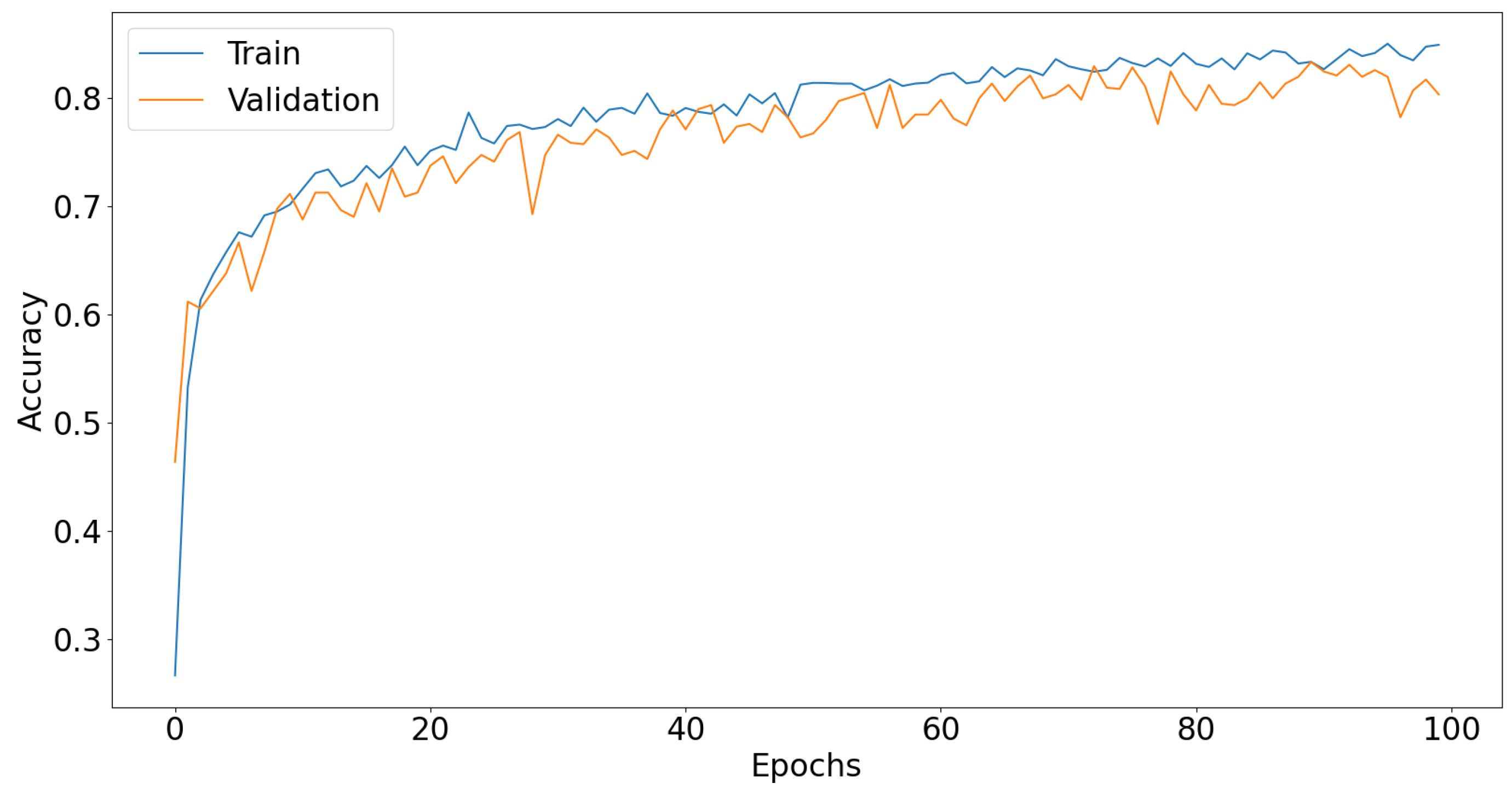
3. Experiments and Results

This section presents the different experiments for the task of identifying Greek Orthodox Church hymns. First, the performance results of the three different CNN models are discussed; then, the comparison with the SOTA pre-trained models is provided. This section is concluded with an analysis of the results.

3.1. Dl Models

The model’s weights update is performed using an Adam (adaptive moment estimation) algorithm [45]. The training process exploits the capabilities of an NVIDIA RTX 3080 GPU. Each base model is trained for 100 epochs with a mini-batch size of 4. The learning rate is set to ${10}^{-4}$, since the experiments with different learning rate formats under-performed. To study the generalization capability of our CNNs, five-fold cross-validation is utilized. The dataset is split in such a way that the training set contains 70% of the initial data, and the validation and the test sets consist of 15% of the initial dataset each. Since five-fold cross-validation is used, each training fold consists of 2892 images. Finally, the same folds are used for all the experiments.

In

Table 2. Models’ computational cost for one forward pass.

Model	Parameters Size (MB)	Number of Parameters	Number of Operations
Shallow CNN	1.36	8,391,191	15.73 M
Deep CNN	2.3	68,660,631	6.42 G
Micro VGG	1.96	489,687	234.6 M

, the computational cost of each custom model is presented. Each model is studied regarding the space it occupies in terms of Megabytes, the number of parameters that need to be updated after each training epoch, and finally the number of multiplications and additions that need to be performed in a single forward pass. In

Table 3. Models’ performance: Accuracy.

Model	Train Accuracy %	Validation Accuracy %	Test Accuracy %
Shallow CNN	83.33 ± 1.24	83.52 ± 0.83	82.79
Deep CNN	95.99 ± 1.28	96.10 ± 0.89	94.01
Micro VGG	97.16 ± 1.19	97.14 ± 0.74	96.38

,

Table 4. Models’ performance: Statistical metrics.

Model	Precision	Recall	F1-Score
Shallow CNN	0.83	0.82	0.83
Deep CNN	0.95	0.96	0.95
Micro VGG	0.97	0.97	0.97

and

Table 5. Models’ performance: Training and inference time.

Model	Training Time (s)	Inference Time (s)
Shallow CNN	1937.002	3.88
Deep CNN	3405.890	4.79
Micro VGG	2091.434	4.02

, the performance of the proposed approaches is presented, while the training and validation loss and accuracy are shown in Figure 4, Figure 5, Figure 6, Figure 7, Figure 8 and Figure 9. As five-fold cross-validation is carried out, the presented values are average values.

The results presented above show that Micro VGG outperforms the other approaches in terms of performance, at a smaller computational cost.

3.2. Transfer Learning—Comparison with SOTA Models

Five different SOTA-pre-trained DL models for audio classification and one for image classification are trained on the same task to further evaluate our models’ performance. More specifically, VGGish, ResNet18 [20], MobileNetV3 [46], SqueezeNet [23], and EfficientNet [47] are trained on the same dataset. As in the previous experiments, the Adam optimizer is used, the learning rate is equal to ${10}^{-4}$, and the same GPU is used. Again, five-fold cross-validation was used to study the generalization of the results.

The computational cost of each model is provided in

Table 6. SOTA models’ computational cost for one forward pass.

Model	Parameters Size (MB)	Number of Parameters	Number of Operations
VGGish	220.48	55,119,447	28.45 G
ResNet18	44.75	11,188,311	148.07 M
MobileNetV3	6.14	1,542,765	240.93 M
SqueezeNet	4.37	734,295	17.26 M
EfficientNet	4.74	4,037,011	7 M

, while the performance is given in

Table 7. Models’ performance.

Model	Train Accuracy %	Validation Accuracy %	Test Accuracy %
VGGish	100 ± 0	98.03 ± 1.16	95.42
ResNet18	96.18 ± 1.21	97.27 ± 1.08	96.11
MobileNetV3	94.87 ± 1.22	98.18 ± 1.03	95.76
SqueezeNet	90.08 ± 1.26	91.04 ± 0.99	88.78
EfficientNet	95.99 ± 1.19	97.14 ± 0.91	96.13

,

Table 8. Models’ performance.

Model	Precision	Recall	F1-Score
VGGish	0.94	0.94	0.94
ResNet18	0.97	0.98	0.97
MobileNetV3	0.96	0.95	0.95
SqueezeNet	0.89	0.89	0.89
EfficientNet	0.96	0.96	0.96

and

Table 9. Models’ performance: Training and inference time.

Model	Training Time (s)	Inference Time (s)
VGGish	3054.258	4.73
ResNet18	2811.133	4.11
MobileNetV3	7813.502	5.89
SqueezeNet	2821.533	4.23
EfficientNet	3018.431	4.67

. The five pre-trained models require large amounts of computational resources, achieving results similar to Micro VGG. However, both ResNet18 and VGGish are more prone to overfitting.

4. Discussion

DL has emerged as a powerful tool in audio signal processing problems. In this work, CV and DL approaches are explored for the task of Greek Orthodox Church hymns identification for mobile applications. Due to the restrictions that are imposed by the low complexity requirement, only lightweight DL models are considered. Three custom CNNs and five SOTA DL models are applied to the task of Greek Orthodox Church hymns identification. The first two custom CNNs employ a conventional structure with both convolution layers and fully-connected layers, while the third one, Micro VGG, is introduced as an improvement of the previous two, incorporating the VGG architecture at a smaller scale. The five pre-trained CNNs are chosen because, in the academic literature, they have been tested for similar problems to ours. The eight DL models are compared both in terms of accuracy and their computational cost. From the analysis of the results, it is evident that Micro VGG outperforms the other approaches in terms of performance, at a smaller computational cost. Batch normalization has improved our model’s performance, while a constant learning rate proved more adequate. Since Micro VGG is considered the best candidate solution for our problem, its confusion matrix is provided in Figure 10. From the heatmap that is represented in the confusion matrix, it is proven that Micro VGG is not biased and classifies all the hymns uniformly.

The findings of our work suggest that it is rather possible to make a mobile app that can be used inside of a church for hymn identification and classification. Such a mobile app will be useful for both tourists and church believers.

Although Micro VGG’s performance is rather satisfactory, our work has certain limitations. First, the dataset is relatively small, affecting the model’s accuracy. Although data augmentation methods are used, more samples per hymn could lead to better results. Furthermore, CNNs are only a class of DL models. Other architectures that are often utilized in audio processing are recurrent neural networks (RNNs) and attention-based models. RNNs are designed for data with sequential structure, like audio, while attention-based models like Transformers have achieved impressive results in fields like NLP and CV. However, RNNs are trained on the audio data themselves so their application requires a different experimental setup [2,48]. Despite their recent success, Transformers still achieve SOTA performance only on large datasets and there are only a few attention-based models that can be considered lightweight [49,50]. In future works, where the largest dataset will be available, both of these DL approaches will be studied for Greek Orthodox Church hymns recognition.

5. Conclusions

In this work, CV and DL methodologies are employed to address the problem of Greek Orthodox Church hymns identification. The goal is to develop DL models suitable for mobile applications. Three approaches are applied to our private dataset; however, a VGG variant achieves the best results. The proposed Micro VGG can identify Greek Orthodox Church hymns with more than 96% accuracy. In addition, Micro VGG outperforms two SOTA models, namely ResNet18, VGGish, MobileNet, SqueezeNet, and EfficientNet, requiring fewer resources. There are still many ways to improve our results, such as by exploiting more data per class, exploring ensemble and federated learning techniques, and utilizing few-shot learning approaches. More specifically, new data samples will be added shortly, updating and expanding our dataset. DL efficiently exploits larger amounts of data; thus, an expanded audio dataset will further improve our results. Ensemble learning is an ML technique that combines multiple learners to construct a stronger one. Such methods could improve overall accuracy. Considering that we desire to apply our method to mobile devices, federated learning, which offers decentralized training, could also be exploited. Finally, few-shot learning or meta-learning allows a learner to learn from other learning algorithms and can be combined with ensemble learning approaches, while it can further mitigate computational costs from edge devices. In our future work, we will develop a mobile app using these DL approaches.

References

1. Fiorucci, M.; Khoroshiltseva, M.; Pontil, M.; Traviglia, A.; Del Bue, A.; James, S. Machine Learning for Cultural Heritage: A Survey. Pattern Recognit. Lett. 2020, 133, 102–108. [Google Scholar] [CrossRef]
2. Purwins, H.; Li, B.; Virtanen, T.; Schlüter, J.; Chang, S.Y.; Sainath, T. Deep Learning for Audio Signal Processing. IEEE J. Sel. Top. Signal Process. 2019, 13, 206–219. [Google Scholar] [CrossRef] [Green Version]
3. Castellano, G.; Vessio, G. Deep learning approaches to pattern extraction and recognition in paintings and drawings: An overview. Neural Comput. Appl. 2021, 33, 12263–12282. [Google Scholar] [CrossRef]
4. Lin, Q.; Ding, B. Music Score Recognition Method Based on Deep Learning. Intell. Neurosci. 2022, 2022. [Google Scholar] [CrossRef] [PubMed]
5. De Vega, F.F.; Alvarado, J.; Cortez, J.V. Optical Music Recognition and Deep Learning: An application to 4-part harmony. In Proceedings of the 2022 IEEE Congress on Evolutionary Computation (CEC), Padua, Italy, 18–23 July 2022; pp. 1–7. [Google Scholar] [CrossRef]
6. Goodfellow, I.; Bengio, Y.; Courville, A. Deep Learning; Adaptive Computation and Machine Learning; MIT Press: Cambridge, MA, USA, 2016; p. 800. [Google Scholar]
7. Nanni, L.; Maguolo, G.; Brahnam, S.; Paci, M. An Ensemble of Convolutional Neural Networks for Audio Classification. Appl. Sci. 2021, 11, 3579. [Google Scholar] [CrossRef]
8. Zhao, T.; Xie, Y.; Wang, Y.; Cheng, J.; Guo, X.; Hu, B.; Chen, Y. A Survey of Deep Learning on Mobile Devices: Applications, Optimizations, Challenges, and Research Opportunities. Proc. IEEE 2022, 110, 334–354. [Google Scholar] [CrossRef]
9. Baldominos, A.; Cervantes, A.; Saez, Y.; Isasi, P. A Comparison of Machine Learning and Deep Learning Techniques for Activity Recognition using Mobile Devices. Sensors 2019, 19, 521. [Google Scholar] [CrossRef] [Green Version]
10. Pérez Arteaga, S.; Sandoval Orozco, A.L.; García Villalba, L.J. Analysis of Machine Learning Techniques for Information Classification in Mobile Applications. Appl. Sci. 2023, 13, 5438. [Google Scholar] [CrossRef]
11. Cano, P.; Batle, E.; Kalker, T.; Haitsma, J. A review of algorithms for audio fingerprinting. In Proceedings of the 2002 IEEE Workshop on Multimedia Signal Processing, St. Thomas, VI, USA, 9–11 December 2002; pp. 169–173. [Google Scholar] [CrossRef]
12. Wang, A.L. An industrial-strength audio search algorithm. In Proceedings of the ISMIR 2003, 4th Symposium Conference on Music Information Retrieval, Baltimore, MA, USA, 27–30 October 2003; pp. 7–13. [Google Scholar]
13. Moysis, L.; Iliadis, L.A.; Sotiroudis, S.P.; Boursianis, A.D.; Papadopoulou, M.S.; Kokkinidis, K.I.D.; Volos, C.; Sarigiannidis, P.; Nikolaidis, S.; Goudos, S.K. Music Deep Learning: Deep Learning Methods for Music Signal Processing—A Review of the State-of-the-Art. IEEE Access 2023, 11, 17031–17052. [Google Scholar] [CrossRef]
14. Schedl, M. Deep Learning in Music Recommendation Systems. Front. Appl. Math. Stat. 2019, 5. [Google Scholar] [CrossRef] [Green Version]
15. Hernandez-Olivan, C.; Beltrán, J.R. Music Composition with Deep Learning: A Review. In Advances in Speech and Music Technology: Computational Aspects and Applications; Springer International Publishing: Cham, Switzerland, 2023; pp. 25–50. [Google Scholar] [CrossRef]
16. Khamparia, A.; Gupta, D.; Nguyen, N.G.; Khanna, A.; Pandey, B.; Tiwari, P. Sound Classification Using Convolutional Neural Network and Tensor Deep Stacking Network. IEEE Access 2019, 7, 7717–7727. [Google Scholar] [CrossRef]
17. Krizhevsky, A.; Sutskever, I.; Hinton, G.E. ImageNet Classification with Deep Convolutional Neural Networks. In Proceedings of the Advances in Neural Information Processing Systems; Pereira, F., Burges, C., Bottou, L., Weinberger, K., Eds.; Curran Associates, Inc.: Red Hook, NY, USA, 2012; Volume 25. [Google Scholar]
18. Szegedy, C.; Liu, W.; Jia, Y.; Sermanet, P.; Reed, S.; Anguelov, D.; Erhan, D.; Vanhoucke, V.; Rabinovich, A. Going deeper with convolutions. In Proceedings of the 2015 IEEE Conference on Computer Vision and Pattern Recognition (CVPR), Boston, MA, USA, 7–12 June 2015; pp. 1–9. [Google Scholar] [CrossRef] [Green Version]
19. Simonyan, K.; Zisserman, A. Very Deep Convolutional Networks for Large-Scale Image Recognition. In Proceedings of the 3rd International Conference on Learning Representations (ICLR 2015), San Diego, CA, USA, 7–9 May 2015; pp. 1–14. [Google Scholar]
20. He, K.; Zhang, X.; Ren, S.; Sun, J. Deep Residual Learning for Image Recognition. In Proceedings of the 2016 IEEE Conference on Computer Vision and Pattern Recognition (CVPR), Las Vegas, NV, USA, 27–30 June 2016; pp. 770–778. [Google Scholar] [CrossRef] [Green Version]
21. Szegedy, C.; Vanhoucke, V.; Ioffe, S.; Shlens, J.; Wojna, Z. Rethinking the Inception Architecture for Computer Vision. In Proceedings of the 2016 IEEE Conference on Computer Vision and Pattern Recognition (CVPR), Las Vegas, NV, USA, 27–30 June 2016; pp. 2818–2826. [Google Scholar] [CrossRef] [Green Version]
22. Hershey, S.; Chaudhuri, S.; Ellis, D.P.W.; Gemmeke, J.F.; Jansen, A.; Moore, R.C.; Plakal, M.; Platt, D.; Saurous, R.A.; Seybold, B.; et al. CNN architectures for large-scale audio classification. In Proceedings of the 2017 IEEE International Conference on Acoustics, Speech and Signal Processing (ICASSP), New Orleans, LA, USA, 5–9 March 2017; pp. 131–135. [Google Scholar] [CrossRef] [Green Version]
23. Iandola, F.N.; Moskewicz, M.W.; Ashraf, K.; Han, S.; Dally, W.J.; Keutzer, K. SqueezeNet: AlexNet-level accuracy with 50x fewer parameters and <0.5MB model size. arXiv 2016, arXiv:1602.07360. [Google Scholar]
24. Ma, N.; Zhang, X.; Zheng, H.T.; Sun, J. ShuffleNet V2: Practical Guidelines for Efficient CNN Architecture Design. In Proceedings of the European Conference on Computer Vision (ECCV), Munich, Germany, 8–14 September 2018. [Google Scholar]
25. Tsalera, E.; Papadakis, A.; Samarakou, M. Comparison of Pre-Trained CNNs for Audio Classification Using Transfer Learning. J. Sens. Actuator Netw. 2021, 10, 72. [Google Scholar] [CrossRef]
26. Gemmeke, J.F.; Ellis, D.P.W.; Freedman, D.; Jansen, A.; Lawrence, W.; Moore, R.C.; Plakal, M.; Ritter, M. Audio Set: An ontology and human-labeled dataset for audio events. In Proceedings of the 2017 IEEE International Conference on Acoustics, Speech and Signal Processing (ICASSP), New Orleans, LA, USA, 5–9 March 2017; pp. 776–780. [Google Scholar] [CrossRef]
27. Green, M.; Murphy, D. Environmental sound monitoring using machine learning on mobile devices. Appl. Acoust. 2020, 159, 107041. [Google Scholar] [CrossRef]
28. Ryumin, D.; Ivanko, D.; Ryumina, E. Audio-Visual Speech and Gesture Recognition by Sensors of Mobile Devices. Sensors 2023, 23, 2284. [Google Scholar] [CrossRef]
29. Tan, K.; Zhang, X.; Wang, D. Deep Learning Based Real-Time Speech Enhancement for Dual-Microphone Mobile Phones. IEEE/ACM Trans. Audio Speech, Lang. Process. 2021, 29, 1853–1863. [Google Scholar] [CrossRef]
30. Farajzadeh, N.; Sadeghzadeh, N.; Hashemzadeh, M. PMG-Net: Persian music genre classification using deep neural networks. Entertain. Comput. 2023, 44, 100518. [Google Scholar] [CrossRef]
31. Sharma, D.; Taran, S.; Pandey, A. A fusion way of feature extraction for automatic categorization of music genres. Multimed. Tools Appl. 2023. [Google Scholar] [CrossRef]
32. Müller, S.G.; Hutter, F. TrivialAugment: Tuning-Free Yet State-of-the-Art Data Augmentation. In Proceedings of the IEEE/CVF International Conference on Computer Vision (ICCV), Virtual, 1–17 October 2021; pp. 774–782. [Google Scholar]
33. Zhang, H.; Cisse, M.; Dauphin, Y.N.; Lopez-Paz, D. mixup: Beyond Empirical Risk Minimization. In Proceedings of the International Conference on Learning Representations, Vancouver, BC, Canada, 30 April–3 May 2018. [Google Scholar]
34. Park, D.S.; Chan, W.; Zhang, Y.; Chiu, C.C.; Zoph, B.; Cubuk, E.D.; Le, Q.V. SpecAugment: A Simple Data Augmentation Method for Automatic Speech Recognition. Interspeech 2019. [Google Scholar] [CrossRef] [Green Version]
35. Li, Z.; Liu, F.; Yang, W.; Peng, S.; Zhou, J. A Survey of Convolutional Neural Networks: Analysis, Applications, and Prospects. IEEE Trans. Neural Netw. Learn. Syst. 2022, 33, 6999–7019. [Google Scholar] [CrossRef]
36. Srivastava, N.; Hinton, G.; Krizhevsky, A.; Sutskever, I.; Salakhutdinov, R. Dropout: A Simple Way to Prevent Neural Networks from Overfitting. J. Mach. Learn. Res. 2014, 15, 1929–1958. [Google Scholar]
37. Ioffe, S.; Szegedy, C. Batch Normalization: Accelerating Deep Network Training by Reducing Internal Covariate Shift. In Proceedings of the 32nd International Conference on Machine Learning, Lille, France, 7–9 July 2015; Volume 37, pp. 448–456. [Google Scholar]
38. Santurkar, S.; Tsipras, D.; Ilyas, A.; Madry, A. How Does Batch Normalization Help Optimization? In Proceedings of the Advances in Neural Information Processing Systems; Bengio, S., Wallach, H., Larochelle, H., Grauman, K., Cesa-Bianchi, N., Garnett, R., Eds.; Curran Associates, Inc.: Red Hook, NY, USA, 2018; Volume 31. [Google Scholar]
39. Yang, G.; Pennington, J.; Rao, V.; Sohl-Dickstein, J.; Schoenholz, S.S. A Mean Field Theory of Batch Normalization. In Proceedings of the International Conference on Learning Representations, New Orleans, LA, USA, 6–9 May 2019. [Google Scholar]
40. Glorot, X.; Bengio, Y. Understanding the difficulty of training deep feedforward neural networks. In Proceedings of the Thirteenth International Conference on Artificial Intelligence and Statistics, Sardinia, Italy, 13–15 May 2010; Volume 9, pp. 249–256. [Google Scholar]
41. Hand, D.; Till, R. A Simple Generalisation of the Area Under the ROC Curve for Multiple Class Classification Problems. Mach. Learn. 2001, 45, 171–186. [Google Scholar] [CrossRef]
42. Grandini, M.; Bagli, E.; Visani, G. Metrics for Multi-Class Classification: An Overview. arXiv 2020, arXiv:2008.05756. [Google Scholar] [CrossRef]
43. Sokolova, M.; Lapalme, G. A systematic analysis of performance measures for classification tasks. Inf. Process. Manag. 2009, 45, 427–437. [Google Scholar] [CrossRef]
44. Russakovsky, O.; Deng, J.; Su, H.; Krause, J.; Satheesh, S.; Ma, S.; Huang, Z.; Karpathy, A.; Khosla, A.; Bernstein, M.; et al. ImageNet Large Scale Visual Recognition Challenge. Int. J. Comput. Vis. (IJCV) 2015, 115, 211–252. [Google Scholar] [CrossRef] [Green Version]
45. Kingma, D.P.; Ba, J. Adam: A Method for Stochastic Optimization. In Proceedings of the 3rd International Conference on Learning Representations—ICLR 2015, San Diego, CA, USA, 7–9 May 2015. [Google Scholar]
46. Howard, A.G.; Sandler, M.; Chu, G.; Chen, L.C.; Chen, B.; Tan, M.; Wang, W.; Zhu, Y.; Pang, R.; Vasudevan, V.; et al. Searching for MobileNetV3. In Proceedings of the 2019 IEEE/CVF International Conference on Computer Vision (ICCV), Seoul, Republic of Korea, 27 October–2 November 2019; pp. 1314–1324. [Google Scholar]
47. Tan, M.; Le, Q. EfficientNet: Rethinking Model Scaling for Convolutional Neural Networks. In Proceedings of the 36th International Conference on Machine Learning, Long Beach, CA, USA, 9–15 June 2019; Volume 97, pp. 6105–6114. [Google Scholar]
48. Gimeno, P.; Viñals, I.; Ortega, A.; Miguel, A.; Lleida, E. Multiclass audio segmentation based on recurrent neural networks for broadcast domain data. EURASIP J. Audio, Speech, Music Process. 2020, 2020. [Google Scholar] [CrossRef] [Green Version]
49. Han, K.; Wang, Y.; Chen, H.; Chen, X.; Guo, J.; Liu, Z.; Tang, Y.; Xiao, A.; Xu, C.; Xu, Y.; et al. A Survey on Vision Transformer. IEEE Trans. Pattern Anal. Mach. Intell. 2023, 45, 87–110. [Google Scholar] [CrossRef]
50. Xu, P.; Zhu, X.; Clifton, D.A. Multimodal Learning With Transformers: A Survey. IEee Trans. Pattern Anal. Mach. Intell. 2023, 1–20. [Google Scholar] [CrossRef]
Figure 1. Boxplot for each hymn of our dataset.
Applsci 13 08638 g001
Figure 2. Examples of four different Mel-spectrograms from our private dataset.
Applsci 13 08638 g002
Figure 3. DL models architecture: (a) Shallow CNN, (b) Deep CNN, and (c) Micro VGG.
Applsci 13 08638 g003
Figure 4. Shallow CNN performance: Accuracy.
Applsci 13 08638 g004
Figure 5. Shallow CNN performance: Loss.
Applsci 13 08638 g005
Figure 6. Deep CNN performance: Accuracy.
Applsci 13 08638 g006
Figure 7. Deep CNN performance: Loss.
Applsci 13 08638 g007
Figure 8. Micro VGG performance: Accuracy.
Applsci 13 08638 g008
Figure 9. Micro VGG performance: Loss.
Applsci 13 08638 g009
Figure 10. Micro VGG confusion matrix.
Applsci 13 08638 g010