A Multi-Stage Deep Reinforcement Learning with Search-Based Optimization for Air–Ground Unmanned System Navigation

Abstract

An important challenge for air–ground unmanned systems achieving autonomy is navigation, which is essential for them to accomplish various tasks in unknown environments. This paper proposes an end-to-end framework for solving air–ground unmanned system navigation using deep reinforcement learning (DRL) while optimizing by using a priori information from search-based path planning methods, which we call search-based optimizing DRL (SO-DRL) for the air–ground unmanned system. SO-DRL enables agents, i.e., an unmanned aerial vehicle (UAV) or an unmanned ground vehicle (UGV) to move to a given target in a completely unknown environment using only Lidar, without additional mapping or global planning. Our framework is equipped with Deep Deterministic Policy Gradient (DDPG), an actor–critic-based reinforcement learning algorithm, to input the agents’ state and laser scan measurements into the network and map them to continuous motion control. SO-DRL draws on current excellent search-based algorithms to demonstrate path planning and calculate rewards for its behavior. The demonstrated strategies are replayed in an experienced pool along with the autonomously trained strategies according to their priority. We use a multi-stage training approach based on course learning to train SO-DRL on the 3D simulator Gazebo and verify the robustness and success of the algorithm using new test environments for path planning in unknown environments. The experimental results show that SO-DRL can achieve faster algorithm convergence and a higher success rate. We piggybacked SO-DRL directly onto a real air–ground unmanned system, and SO-DRL can guide a UAV or UGV for navigation without adjusting any networks.

1. Introduction

Intelligent robots are playing an indispensable role in various industries [1,2,3], and a wide variety of intelligent robots are ubiquitously showing remarkable availability in transportation, logistics, agricultural development, and disaster emergency response. An unmanned ground vehicle (UGV) can accurately reach a destination to perform tasks, and they are highly superior in engineering expeditions, military reconnaissance, rescue and relief, etc. [4]. They can help humans operate under harsh conditions, but have significant limitations on environmental perception due to their height. In contrast, unmanned aerial vehicles (UAVs), a major research hotspot today [5,6,7,8,9], have the advantages of small size, simple structure, flexible operation, vertical takeoff and landing, and more flexible detection of a wide field of view compared to UGVs.

The use of unmanned air–ground systems, including UAVs and UGVs, has become an important research area [10,11,12] in both military and non-military fields. The potential of unmanned air–ground systems is immeasurable, with predictable and broad applications in hazardous work such as manufacturing, construction, agriculture, hazardous chemical spills, geological disasters, disaster relief, and traffic accidents [13,14,15]. To expand the scope of application scenarios and working capabilities of UGVs/UAVs, it is necessary to improve the autonomous navigation capabilities of unmanned air–ground systems in unknown working environments.

Traditional path planning algorithms for the air–ground unmanned system mainly include A* algorithm [16], ant colony algorithm [17], artificial potential field method [18], genetic algorithm [19], etc. However, in many applications of air–ground unmanned systems, the complex and unpredictable operating environment requires path planning methods to exhibit self-learning, adaptability, and robustness. Similarly, traditional methods cause high computational costs in highly unstructured environments, such as the stochastic dynamic behavior of obstacles and the unknown nature of the environment [20]. To overcome the weaknesses of these methods, multiple solutions have been proposed. Reinforcement learning techniques can learn appropriate actions from environmental states, with benefits based on the concept of online learning and rewards or punishments from the environment, which allows the agent to modify its policy based on the rewards or punishments received. Deep reinforcement learning (DRL) has received much attention in recent years in artificial intelligence due to its end-to-end mapping and label-free interaction with the environment. DRL has been widely used in various fields such as video prediction, target localization, text generation, robotics, machine translation, control optimization, autonomous driving, and text-based games, showing strong adaptation and learning capabilities. Currently, DRL has been well applied to mobile robot path planning problems with important results [21].

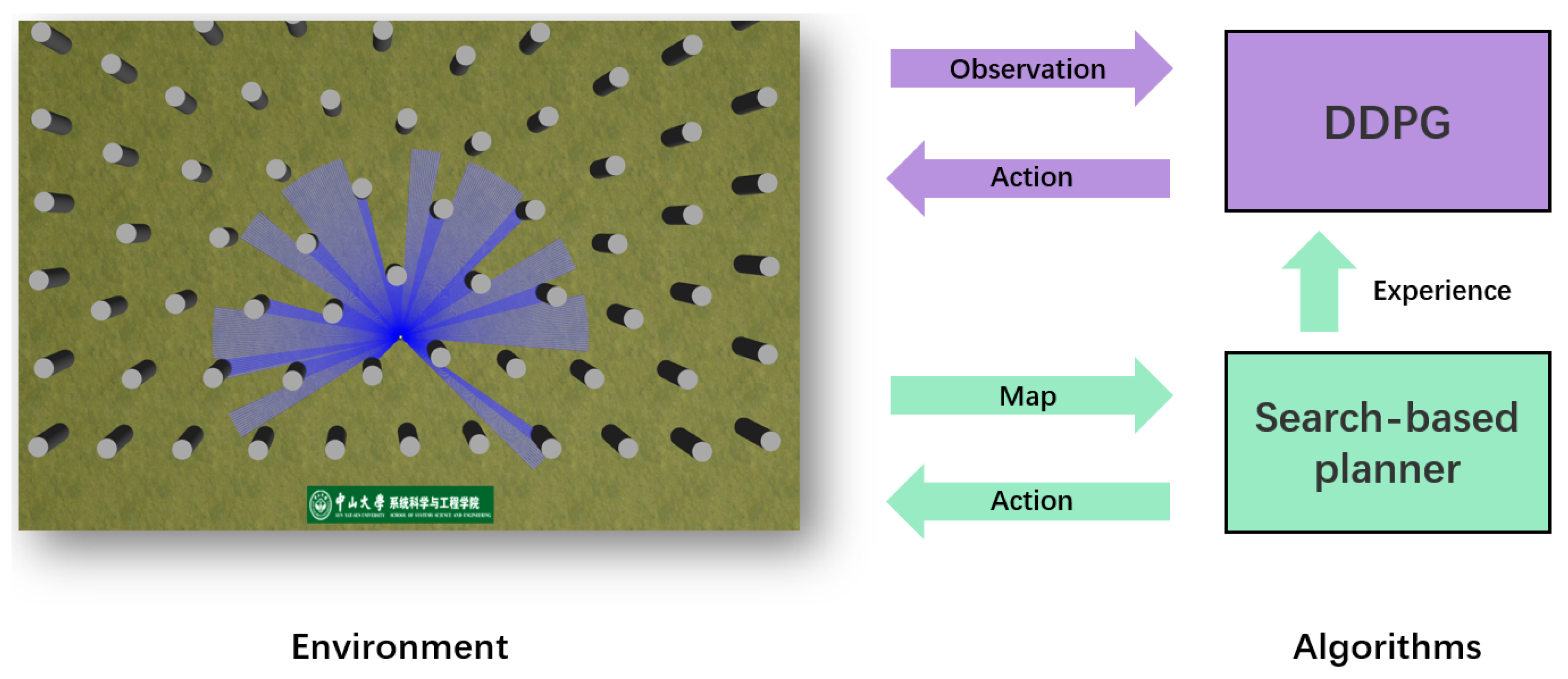
However, when a UGV/UAV employs reinforcement learning to plan a course in an unfamiliar environment, it can only arrive at the optimal solution through trial and error. The applications of search-based path planning have been mature and capable of not only dynamic obstacle avoidance in known environments, but also path optimization for multiple aspects of path smoothing, denoising, and control. Integrating search-based algorithms into reinforcement learning can not only make full use of known information to efficiently learn to accelerate convergence, but also improve the performance of training.

Therefore, based on our previous work [22], this paper proposes an end-to-end path planning framework for air–ground unmanned system navigation, search-based optimizing DRL (SO-DRL), based on the framework of deep reinforcement learning, combined with excellent search-based path planning algorithms. SO-DRL implements Deep Deterministic Policy Gradient (DDPG)-based path planning by piggybacking the search-based algorithm onto the training platform and collecting training experience through the use of known maps for path planning reinforcement learning. The experience is played back according to priority. Eventually, the UGV/UAV equipped with lidar is capable of quickly learning path planning in unknown environments (as shown in Figure 1). The validity of SO-DRL can be verified in a real UGV and UAV without the need to adjust the reference. The main contributions of this paper are the following:

•

A unique end-to-end DRL-based path planning algorithm (SO-DRL) was proposed to enable the air–ground unmanned system to perform path planning obstacle avoidance in unknown environments using only laser perception without the need for known maps and complex path and optimization designs.

•

A priori global optimization of the search-based algorithm was constructed, which alleviated the sparse reward problem at long destination distances and allowed the algorithm to converge quickly and efficiently with better success rate performance.

•

A highly simulated real physical environment was built and a multi-stage learning process based on course learning was designed to quickly and effectively guide the planning of UGV/UAV in more complex environments. The results show that our method has faster, better convergence, and stronger problem-solving ability than classical reinforcement learning methods.

•

Our algorithm has a good generalization capability of simulation to reality. We designed a realistic lidar-only UAV and UGV for obstacle avoidance experiments, which show that the obtained strategies can be mounted on a real UGV or UAV for navigation in unknown environments without optimization.

The remainder of this paper is organized as follows. Section 2 introduces related work. Section 3 models the path planning for reinforcement learning, and the architecture of the developed algorithm. Section 4 discusses the simulation experiment results. Section 5 presents the real-world experiments, and we draw a conclusion and present some potential future work in Section 6.

2. Related Work

SO-DRL uses search-based algorithms to optimize DRL. This section presents the development of the two algorithms and related work of path planning in the air–ground unmanned system, respectively.

2.1. Search-Based Algorithm

The search-based path planning algorithm is a mature path planning algorithm. Based on the established search tree or graph, different search strategies are used to find feasible solutions or even optimal solutions. The basic graph search algorithms for unweighted graphs are Depth First Search (DFS) and Breadth First Search (BFS), both of which are time-for-space methods, with BFS being able to guarantee that the path searched for is optimal. Heuristic search algorithms, such as Greedy Best First Search (GBFS), can improve search efficiency, but cannot ensure that the optimal path is found. Classical algorithms in path planning are Dijkstra, which is an extension of the BFS in a weighted graph, and the A*, which is obtained by adding a heuristic function to the former, taking into account both efficiency and completeness.

Dijkstra, A*, and their improved algorithms such as block A*, D*, field D*, fringe saving A* (FSA*), and generalized adaptive A* (GAA*) [23,24] are efficient search-based algorithms. The work proposed in [25] suggested a Lyapunov-based coordination technique that enables low-level trajectory planning with the A* algorithm. The authors of [26] proposed bidirectional A* algorithms for trajectory planning under intermittent measurements. Additionally, they demonstrated the feasibility and consistency of UAV path planning by utilizing convex hull and B-spline curves. In [27], the authors presented the EBS-A* algorithm, which incorporates extended distance from obstacles, simultaneous search in both directions, and smoothing to reduce right-angle turns in path planning. There is also a class of algorithms such as [6,28,29,30,31,32], which not only accomplishes a good path planning effect but also optimizes the trajectory. Although this kind of algorithm has analytical completeness, when the map dimension is high or the size is large, it needs to process a large amount of data.

2.2. DRL for Path Planning

The ultimate goal of reinforcement learning is to obtain the optimal policy by maximizing the reward value, which has a strong decision-making ability. However, in increasingly complex real-world scenario applications, reinforcement learning cannot solve the dimensional catastrophe problem that arises when the state space is large. In contrast, deep learning has a strong perceptual capability and can be used to extract high-level features from raw large-scale data. DRL [33] combines the decision-making ability of reinforcement learning with the perceptual ability of deep learning, which can directly control based on the input perceptual information and is an artificial intelligence method that is closer to human thinking. Thus, the end-to-end unsupervised training of DRL and its interaction with the environment is well suited to solve navigation problems in unknown environments.

DRL has been successfully used for mobile robot motion planning. TAI et al. [34] proposed a learning-based map-free planner for the case of sparse distance information and no obstacle map, using the 10-dimensional range and the position of the target relative to the robot as input and continuous steering commands as output, and trained the planner using asynchronous deep reinforcement learning methods, so that training and sample collection can be executed in parallel. This method has better stability in extremely complex environments. In [35], the authors proposed a double deep Q-networks (DDQN) technique for controlling IoT data and maximizing data gathering while adhering to flight duration and navigation restrictions without prior knowledge of wireless channel characteristics. The method proposed in [36] learns strategies represented by sequence-to-sequence neural networks with DRL to solve the problem of minimizing the total energy consumption of UAV-IoT system trajectories. In [37], Yan et al. proposed a DRL method for aircraft path planning based on global situational information, utilizing the dueling double deep Q-networks (D3QN) algorithm to solve the path planning problem with situational assessment and taking into account the probability of aircraft survival under enemy radar detection and missile attack. A control strategy based on Deep Deterministic Policy Gradient (DDPG) was proposed by [38] to solve the problem of combining 3D mobility and energy-enhanced multi-vehicle planning, aiming at the problem of energy constraints and the large coverage requirements of communication platforms.

3. Methodology

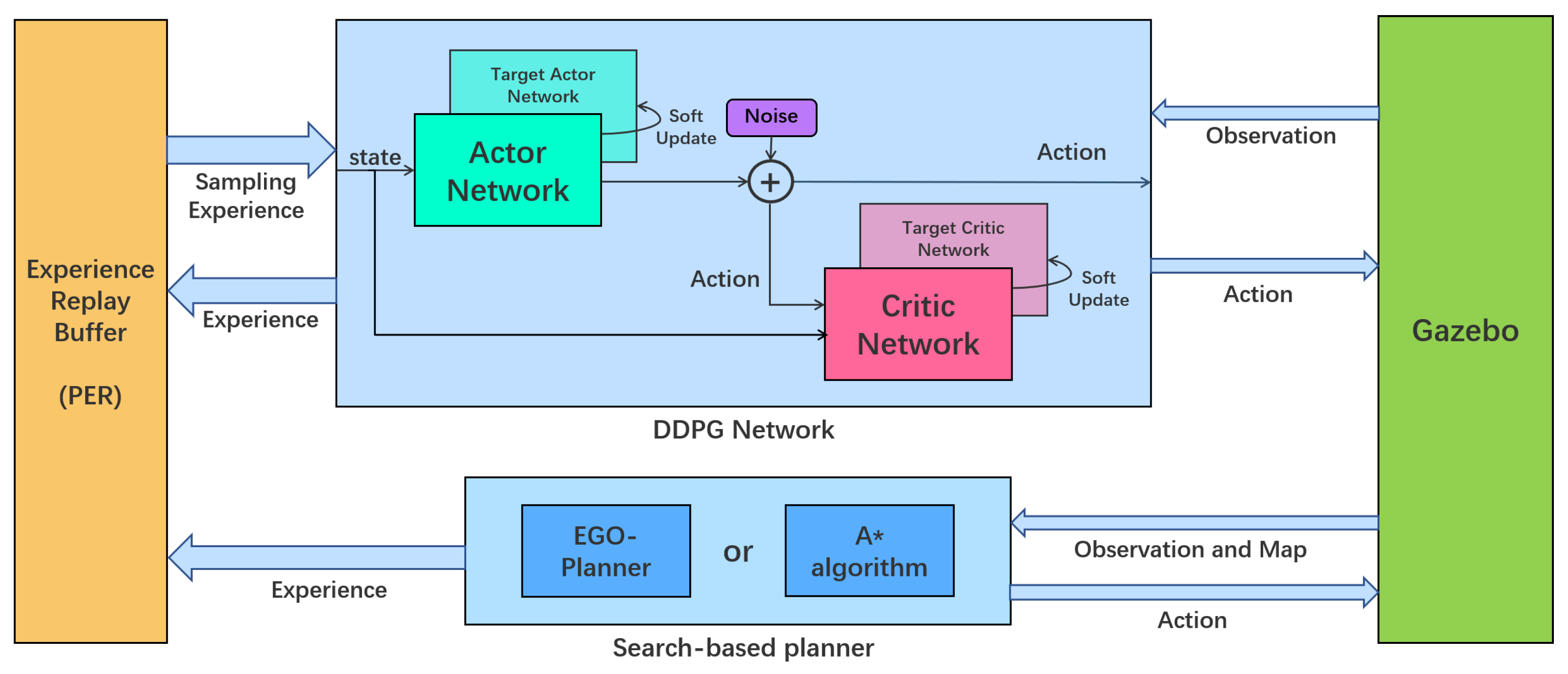
This section describes the implementation of SO-DRL, including Markov’s definition of navigation problem, network design for DRL, optimization approach for search-based methods, and multi-stage course learning training strategy. Our framework is shown in Figure 2.

3.1. Problem Formulation

The path planning problem is defined as finding a collision-free path from a starting position to a target position in an environment with obstacles. In reinforcement learning, the path planning problem can be expressed as a Markov Decision Process (MDP) with the following model: $(S,A,P,R)$ [39]. S denotes the state space, A denotes the action space, P denotes the probability of a state transition, and R denotes the reward function. For path planning, at each discrete time step t, the agent collects the state $s_t\in S$ and selects $a_t\in A$ according to the strategy $\pi$ in the action space. Then, the current state transition to the new state according to the state transition probability $p\left(s_{t+1}\mid s_t,a_t\right)$. Reward $r\left(s_t,a_t\right)$ is given based on the effect of the action. The total reward of a state $R_t$ is defined as the sum of future rewards when considering the future T under the discounting factor $\gamma \in [0,1]$:

$$R_t=\sum _{i=t}^T{\gamma }^{(i-t)}r\left(s_i,a_i\right).$$

(1)

The action-value function describes the expected return following the acquisition of $a_t$ in accordance with $\pi$. As an evaluation index of the current action, it can be expressed recursively as:

$$Q^{\pi }\left(s_t,a_t\right)={\mathbb{E}}_{r_t,s_{t+1}\sim E}\left[r\left(s_t,a_t\right)+\gamma {\mathbb{E}}_{a_{t+1}\sim \pi }\left[Q^{\pi }\left(s_{t+1},a_{t+1}\right)\right]\right].$$

(2)

The task of reinforcement learning is to maximize the Q, i.e., to seek the most profitable action in the current state.

3.2. Reinforcement Learning Setup

In this subsection, we describe the Reinforcement Learning setup. We design the structure and detailed parameters of the deep reinforcement learning network, including the sensor-based observation space, the continuous action space that matches reality, the carefully designed reward function, and the network design for DDPG.

3.2.1. Observation Space

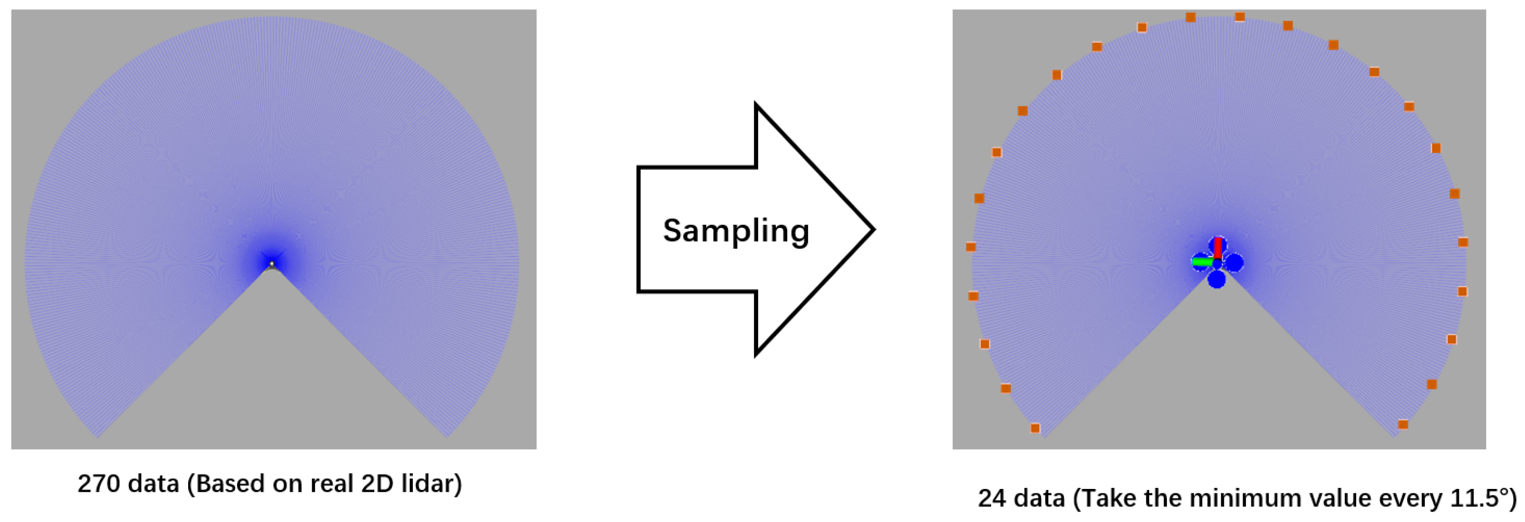
The observation $s_t$ consists of the normalized laser data, the velocity of the agent, and the relative goal position. The laser data is based on a real 2D lidar (Hokuyo UST-10LX: https://www.hokuyo-aut.jp/ (accessed on 20 December 2022)) with a range of 270° and 0.25° resolution. Specifically, the collected raw laser data is sampled as 24 dimensions (as shown in Figure 3) and normalized by its maximum value. The observed velocity includes the current translational and rotational velocity. The relative goal position is calculated in the polar coordinate (distance and angle) with the position of the agent.

3.2.2. Action Space

Since our environment is based on the real world, the control variables of the agent are also continuously controlled to achieve near-real control and facilitate portability in physical objects. The agent adopts a control mode that controls the translational velocity and rotational velocity $A\sim a_t\left[v_t,{\omega }_t\right]$. At each decision, the agent chooses the current action to perform according to the policy network. Considering the real-world safety for the UAV and UGV, we set the range of translational velocity to $v\sim (0,1)$ and the rotational velocity to $\omega \sim (-1,1)$. The agent is not allowed to move backwards $(v\nless 0)$ because the laser does not cover the back area. For the real action output, we add a certain randomness to ensure that the algorithm is exploratory, that is the agent will choose a completely random action according to a certain probability, and for the actions of network decisions, we add random noise to them.

3.2.3. Reward Design

We design the reward function from three aspects to avoid obstacles in the process of reaching the goal and make the action smooth. The composition of reward r is:

$$r=r_g+r_c+r_s+r_a,$$

(3)

where $r_g$ is reaching goal reward, $r_c$ is the collision avoidance reward, $r_s$ is action smoothing reward, and $r_a$ is action urge reward.

The arrival reward guides the agent to approach the goal, which consists of the arrival reward and the distance target approaching reward:

$$r_g=\left\{\begin{array}{cc}{r}_{arrived}\hfill & if∥p_t-p_g∥<d_{min}\hfill \\ \alpha \left(∥p_{t-1}-p_g∥-∥p_t-p_g∥\right)\hfill & \mathrm{otherwise}\hfill \end{array}\right.,$$

(4)

where $r_{\mathit{arrived}}$ is the reward for reaching the goal, $p_t$ is current position of the agent, $p_g$ is the position of goal, $d_{min}$ is the distance to judge the arrival, and $\alpha$ is a constant. If the distance between the position of the agent and goal is within $d_{min}$, it is determined that it has reached the goal, giving the arrival reward $r_{arrived}$. If the agent has not arrived, according to the distance between the current position and the goal and the same distance at the previous moment, we calculate the distance difference close to the target point, and perform $\alpha$ weighting as a reward for approaching the target point.

Collision avoidance reward guides the agent away from obstacles:

$$r_c=\left\{\begin{array}{cc}2r_{collision}\hfill & \mathrm{if}∥p_t-O_k∥<R\hfill \\ r_{collision}\hfill & \mathrm{if}R⩽∥p_t-O_k∥<2R\hfill \\ r_{\mathit{laser}}\hfill & \mathrm{otherwise}\hfill \end{array}\right.,$$

(5)

where $r_{collision}$ is collision warning reward, $O_k(0\le k\le N)$ is the position of obstacle, R is collision distances, and $r_{laser}$ is laser distance reward. If the distance is less than R, it is determined as a collision and a collision penalty of $2r_{collision}$ is given. If the distance is less than $2R$, a collision warning penalty $r_{collision}$ is given. For other cases, the laser judges the openness in the direction of travel, and the penalty $r_{laser}$ is given by the normalized laser.

Action smoothing reward guides the agent to move smoother:

$$r_s=\left\{\begin{array}{cc}r\hfill & \mathrm{if}∥v_t-v_{t-1}∥>v_{min}\hfill \\ 0\hfill & \mathrm{otherwise}\hfill \end{array}+\left\{\begin{array}{cc}{r}_{\omega }& \mathrm{if}∥{\omega }_t-{\omega }_{t-1}∥>{\omega }_{min}\hfill \\ 0& \mathrm{otherwise}\hfill \end{array}\right.\right.,$$

(6)

where $r_v$ is translational velocity smoothing reward, $v_t$ is current translational velocity, $v_{min}$ is translational velocity variation limitation, $r_{\omega }$ is rotational velocity smoothing reward, ${\omega }_t$ is current rotational velocity, and ${\omega }_{min}$ is translational velocity variation limitation. When the change in velocity between the previous moment ($v_{t-1}$ or ${\omega }_{t-1}$) and this moment ($v_t$ or ${\omega }_t$) is greater than $v_{min}$ or ${\omega }_{min}$, the corresponding velocity penalty $r_v$ or $r_{\omega }$ is given.

Action urge reward prevents the agent from stopping in place or moving too slowly:

$$r_a=\left\{\begin{array}{cc}{r}_{uv}\hfill & \mathrm{if}{v}_t<v_{umin}\hfill \\ 0\hfill & \mathrm{otherwise}\hfill \end{array}\right.,$$

(7)

where $r_{uv}$ is translational velocity urge reward and $v_{umin}$ is translational velocity limit. If the translational velocity is less than the minimum velocity limit $v_{umin}$, a penalty $r_{uv}$ is given for moving too slowly.

We set $d_{min}=0.25$, $r_{\mathit{arrived}}=100$, $\alpha =420$, $R=0.25$, $r_{\mathit{collison}}=-100$, $r_v=r_{\omega }=-2$, $v_{min}={\omega }_{min}=0.5$, $r_{uv}=-2$, $v_{\mathit{umin}}=0.2$ in the training.

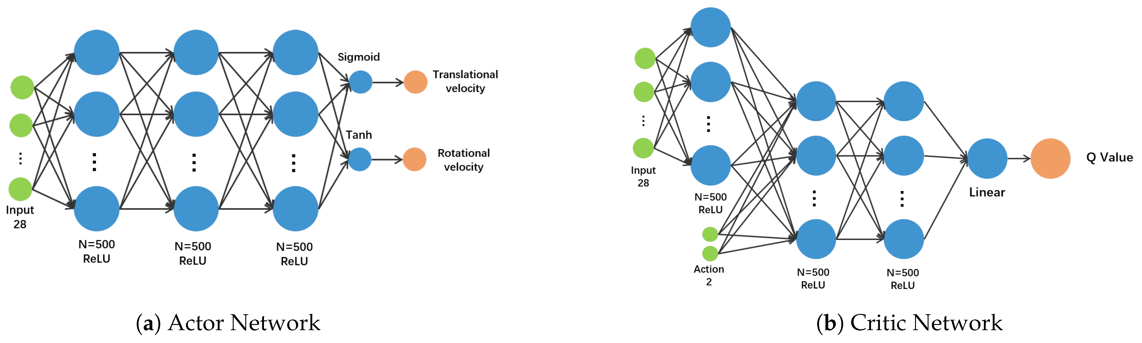
3.2.4. DRL Network Architecture

The DDPG network is an actor–critic, model-free algorithm that can be applied to continuous action spaces. The algorithm uses the actor network to output the continuous spatial action in the random process of the $\pi$ strategy and uses the critic network to calculate the corresponding Q value for the action. Policy replay is performed with an experience replay buffer, from which data is drawn each training session. Both networks have a target network to reduce the impact of network parameter updates on learning stability. The soft update rules of the target networks are:

$$\begin{array}{c}{\theta }^{Q^{\prime }}\leftarrow \tau {\theta }^Q+(1-\tau ){\theta }^{Q^{\prime }}\\ {\theta }^{{\mu }^{\prime }}\leftarrow \tau {\theta }^{\mu }+(1-\tau ){\theta }^{{\mu }^{\prime }}\end{array},$$

(8)

where $\theta$ is the weight of the network, Q stands for the critic network, $Q^{\prime }$ stands for the target critic network, $\mu$ stands for the actor network, and ${\mu }^{\prime }$ stands for the target actor network. $\tau$ is the discount factor, which we set at 0.01 in training.

We elaborate the network as shown in Figure 4. We use the multilayer feedforward neural network [40] to complete the mapping from the input to the output. Actor network maps observation data to actions. We design a 5-hidden-layer neural network as a non-linear function approximator to the policy $\pi$. The first three layers are fully connected networks with 500 rectifier units and ReLU activation functions. Then the full connection outputs the rotational velocity through the Tanh activation function with range $(-1,1)$, and the normalized value $(0,1)$ of the translational velocity through the Sigmoid activation function. Critic network maps observation data and actions to Q-values. After the observation data passes through a fully connected layer, it is merged with the current action. After two fully connected layers, the Q value is output through linear activation.

3.3. Search-Based Optimization

To take advantage of the search-based method, we use it as a demonstration to put data into an experienced pool in the same format as reinforcement learning approaches. In this way, DDPG has advantageous learning samples in the early stage of learning. The experiences of search-based method planning and self-learning are also in the experience replay buffer of DDPG, and normal random extraction cannot guarantee that the advantages of the search-based method can be learned every time. As experience increases, early search-based method data may even be taken out of the buffer. In order to improve the utilization of effective experience, we add a Prioritized Experience Replay (PER) [41] mechanism. PER enables efficient propagation of reward information [42], which is critical for training in the initial stage under training sparse rewards. PER sets the agent’s experience priority so that it takes more important samples from its replay buffer more frequently.

Priority is set with four parameters. Set ${\epsilon }_d$ as a constant that boosts the priority of good experience to increase the probability of being sampled. Although the priority exists, in order to guarantee the generalization performance of the learning, it is necessary to ensure that every experience can be sampled. So, adding small constants $\epsilon$ enables all experiences to be sampled with some probability. The last TD error $\delta$ in the conversion process should also be considered. Finally, join the loss of the network which can be expressed as the gradient descent of the action-value function $J\left(\theta \right)={\nabla }_{a}Q\left(s_i,a_i\mid {\theta }^Q\right)$ and weigh it using $\lambda$. The priority of the experience is calculated as:

$$p_i={\epsilon }_d+\epsilon +{\delta }_i^2+\lambda {\left|J\left(\theta \right)\right|}^2.$$

(9)

Then, the probability that the experience is sampled can be calculated as:

$$P\left(i\right)=\frac{p_i^{\alpha }}{{\sum }_k{p}_k^{\alpha }},$$

(10)

where $P\left(i\right)$ is the sampling probability, $p_i$ is the priority, and $\alpha$ is the distribution factor. Changes in sampling probability also affect the network. To account for the change in the distribution, updates to the network are weighted with importance sampling weights:

$$w_i={\left(\frac{1}{N}·\frac{1}{P\left(i\right)}\right)}^{\beta },$$

(11)

where N is the batch size and $\beta$ is a constant value for adjusting the sampling weights.

The data from the search-based method and the data from autonomous training are prioritized according to the above rules, which can naturally control the ratio of data sampling between the two during the training process, and efficiently utilize the advantages of the search-based method.

We choose two representative search-based methods, A* algorithm and EGO-Planner [29]. A* algorithm provides a basic solution to path planning and intuitively demonstrates the advantages of SO-DRL over unoptimized methods. The EGO-Planner contains more optimizations for real physical motion, which allows SO-DRL to achieve impressive performance.

3.3.1. A* Algorithm Optimization

A* algorithm is a classical and reliable heuristic search algorithm. Through the heuristic function, the value of each extended search node is evaluated comprehensively, the most promising extended point is selected, and the target node is finally found. Since the node with the lowest estimated value is used as the extended node each time, a stable optimal path can be selected.

The A* algorithm is very reliable as an optimization algorithm. First, in our framework, the reliability of the optimization algorithm and its stability in the real world are primary considerations. Our algorithm only learns traditional algorithms from external performance in the early stage, but all decisions are implemented through our framework and are not influenced by other algorithms in memory at all. Second, for the A* algorithm, although the A* algorithm sacrifices spatial complexity, we strongly agree with the accuracy of the A* algorithm and its reliability in practical use. It is also shown in [43] that the tree-search version of A* is optimal if h(n) is admissible, while the graph-search version is optimal if h(n) is consistent. In many practical uses, especially for A* algorithm is very reliable and common in many practical uses, especially for the real physical movement space problem of UAVs and UGVs.

3.3.2. EGO-Planner Optimization

The EGO-Planner explicitly constructs an objective function to keep the trajectory away from obstacles, and the self-planner reduces a significant amount of computation time compared to ESDF-based planners [28,31]. It first parameterizes the trajectory by a uniform b-sample curve and then optimizes it using smoothing penalty, collision penalty, and feasibility penalty terms. In addition, it has an additional individual time redistribution procedure to ensure dynamic feasibility and generate a locally optimal collision-free path for unknown individual obstacles. We select EGO-Planner as a search-based method. EGO-Planner is a state-of-the-art motion planning method for the UAV. In EGO-Planner, the collision-free path is searched by the A* method and optimized by the gradient-based spline optimizer using smoothness, collision, and dynamic feasibility terms. We use globally to plan and optimize trajectories, implementing EGO-Planer onto our platform. To take full advantage of the achievable information, we generate a global point cloud for planning.

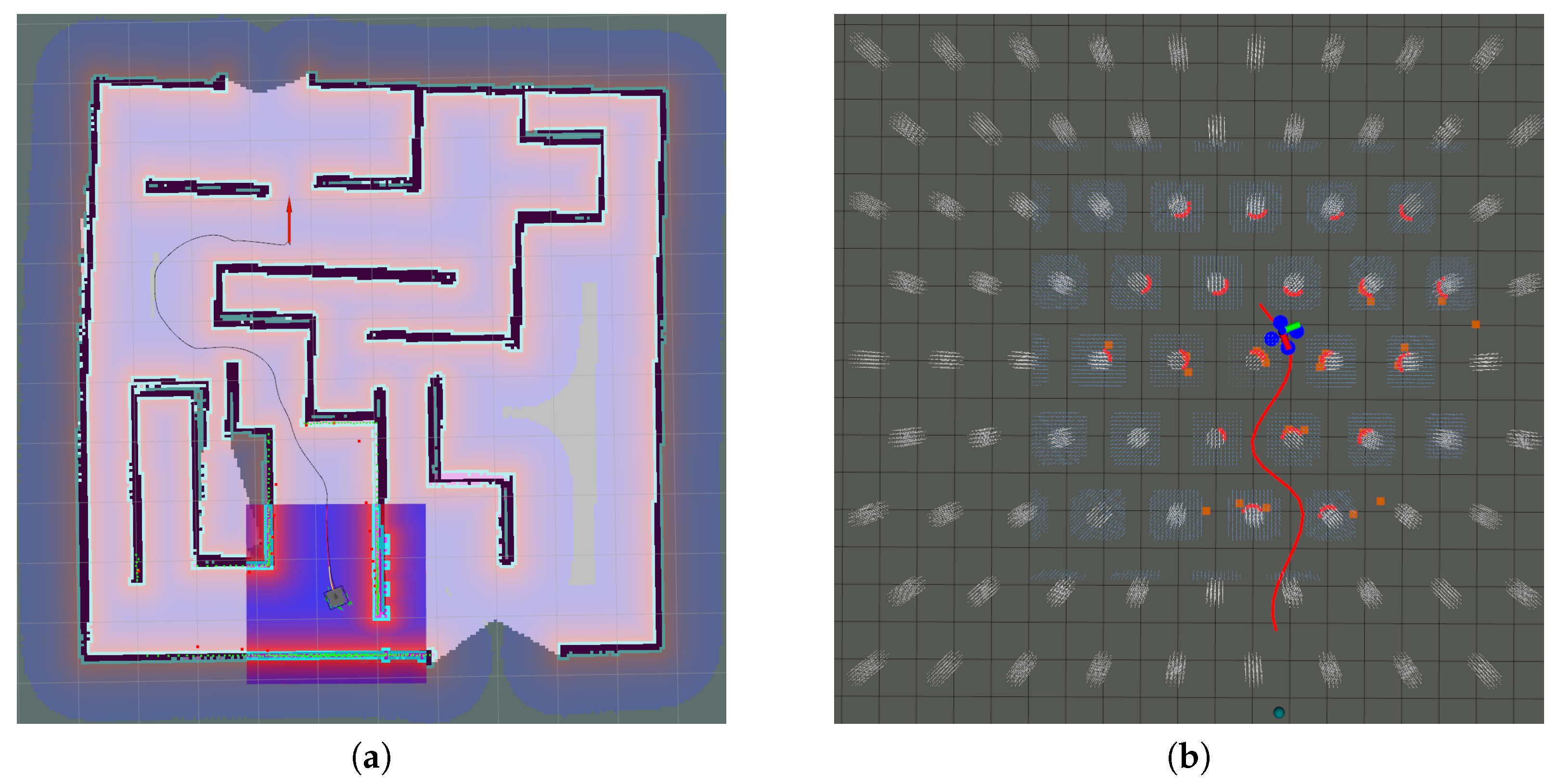
The collection process is shown in Figure 5, while search-based methods require complex computational processes, in the reinforcement learning framework, we only collect observation states (laser information, goal, and velocity) and actions during the planning process. Action rewards are calculated according to the same reward function. Then, this data will enter the experience buffer for priority replay. For the reinforcement learning process, this part of the data is very beneficial to the weight update in the end-to-end implicit learning process.

3.4. Multi-Stage Training

Due to the obstacles being dense and the endpoint being far away, it is difficult to reach the goal in the early stage of the experiment. The DRL can only converge after a long trial and error process. Inspired by curriculum learning [44] in machine learning, we designed the experiment as a multi-stage training process for the path planning problem. Similar to [37,45], we solved the difficulties of the agent in the exploration stage from the perspective of curriculum learning, so that the agent can learn step by step.

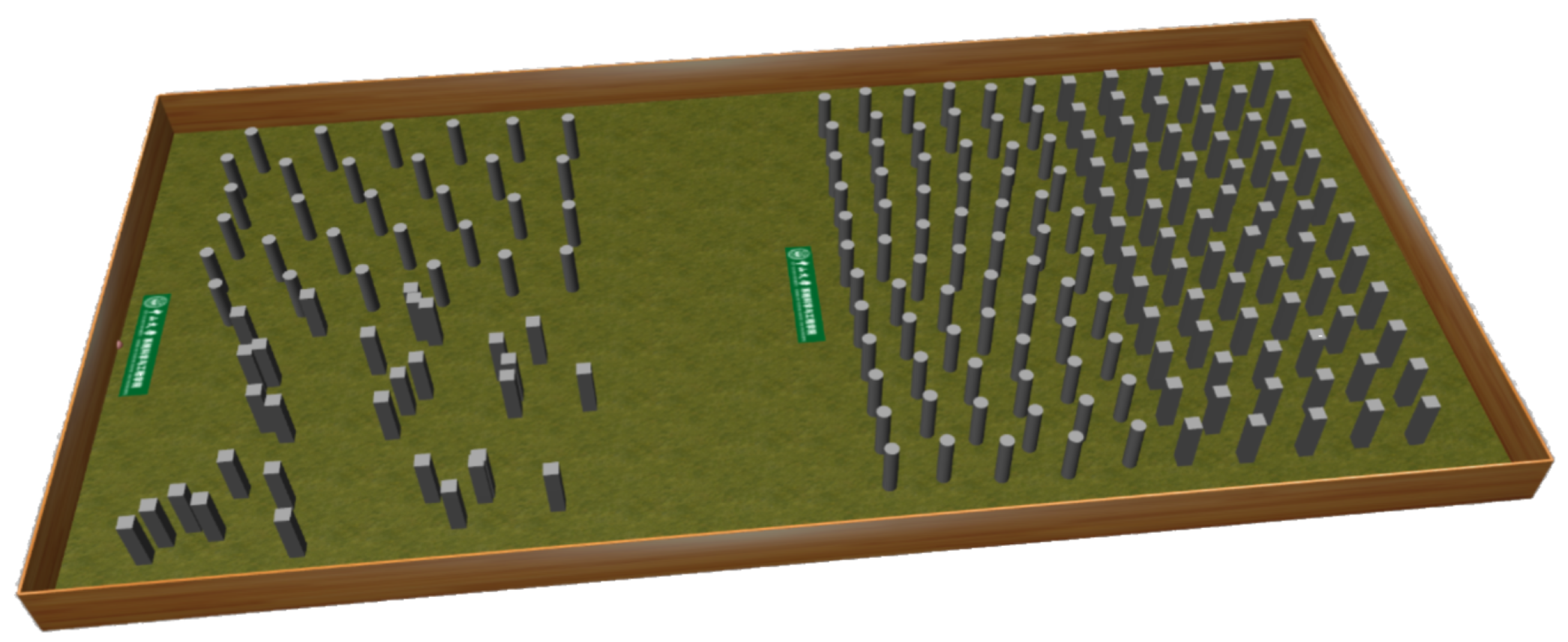
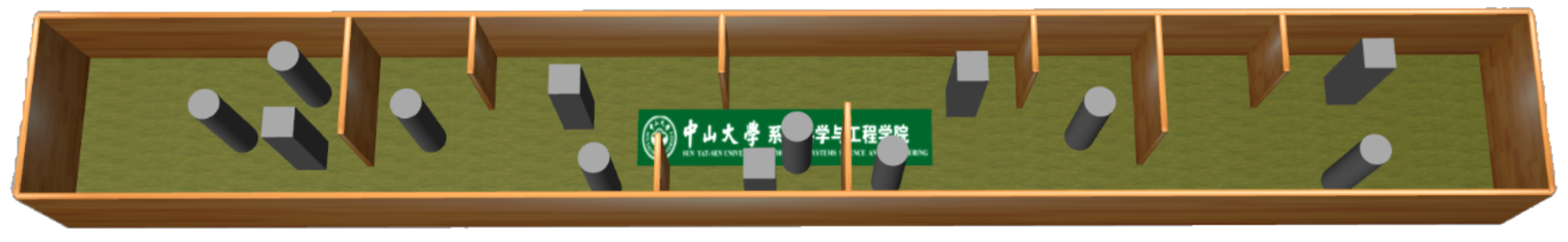
In stage 1, we trained in a sparse obstacle environment with a target distance of 17 m (as shown on the left side of Figure 6), with regularly distributed cylindrical obstacles on the left 10 m × 15 m and randomly distributed square column obstacles on the right 10 m × 15 m, with a buffer space of 1m above and below. This stage of training enabled the agent to complete relatively simple obstacle avoidance tasks quickly and clearly. In the second stage, we set up a dense obstacle environment with a target distance of 22 m (as shown on the right side of Figure 6), containing a total of 140 cylindrical and square column obstacles with a buffer space of 1 m above and below. All the regular arrangement obstacles are generated by K-means approximation. During the training process, once the agent reached reliable performance, we terminated stage 1 and kept the trained strategy, replacing it with stage 2.

4. Simulation Experiments

Simulation experiments were carried out in the semi-physical simulation environment Gazebo. In this section, we will introduce the details of our platform, display and analyze the training results, and show how each algorithm performs in a test environment.

4.1. Experiments Platform

Our experiments were performed on a computer with an Intel Core i7-8700K CPU (Intel, Santa Clara, CA, USA) and an Nvidia GTX 1650 GPU(Nvidia, Santa Clara, CA, USA). The experiments ran on the Ubuntu system, while the robot-related components made use of the ROS (https://www.ros.org/ accessed on 20 December 2022)) and the machine learning-related components made use of the Keras (https://keras.io/ accessed on 20 December 2022)) based on TensorFlow (https://www.tensorflow.org/ accessed on 20 December 2022)). It takes about three hours for a thousand episodes. SO-DRL is a model-free algorithm and we define the UGV/UAV as a prime point for training and testing of the simulation. We used a UAV model instead of a prime point for easy viewing in the simulation. We used an open-source autonomous software platform Prometheus (https://github.com/amov-lab/Prometheus accessed on 20 December 2022)), which supports simulation and experiments with the Gazebo interface.

For environments during training, we generated obstacles (in Figure 6) in the initial stage and create two training scenarios. The learning rate was set to 0.0001 in the experiments. The work proposed in [46] is a seminal paper on deep reinforcement learning, and two ways are given in the paper for evaluating the performance of reinforcement learning algorithms. One is the average score, which averages all the reward values obtained by the agent, showing how correct the algorithm’s action selection is for achieving the purpose. The other is the average Q-value, which averages the actions’ Q-values and shows the algorithm’s reliability in selecting the correct action. Since the paper [46] is the pioneering work of deep reinforcement learning, most subsequent papers use it as a reference. These two metrics have become the performance evaluation metrics for reinforcement learning research. In this paper, the average reward and the average Q-value are also used as evaluation metrics for the network in training, and we take their average in each episode.

We trained SO-DRL in the two scenarios, as shown in Figure 6. The learning rate in the experiments was set to 0.0001. The performance metrics for training include the average reward per set, the average q-value per set, and the success rate computed per 50 sets.

4.2. Evaluation for Multi-Stage Training

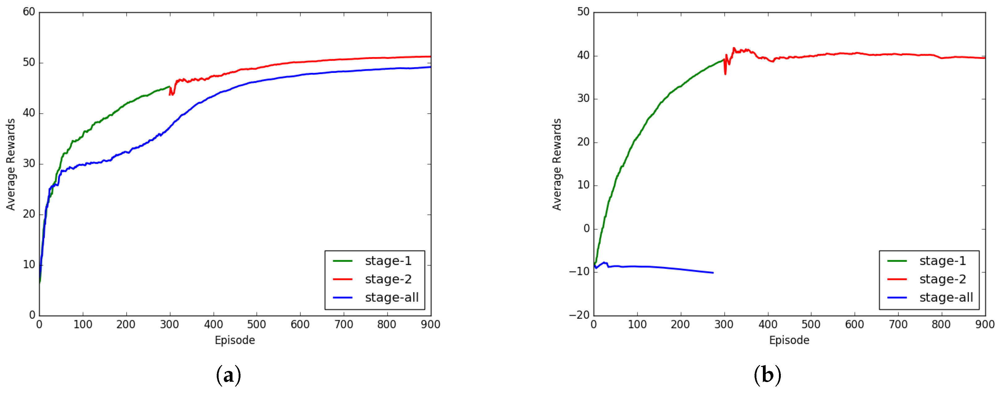
Here, we verify the validity of the proposed multi-stage learning. The agent is first trained in the environment of the first stage. When the training converges, we select the weight of the convergence point as the initial weight for the next stage of training. The effect of the training process is shown in Figure 7.

The effect of our multi-stage training is shown in Figure 7. We performed multi-stage training and one-step training (in Figure 6 right) with SO-DRL(EGO) and DDPG. As can be seen (in Figure 7a), the SO-DRL with a multi-stage learning process accelerated the convergence of the strategy to a satisfactory solution and achieved a higher reward than the strategy trained from scratch for the same number of periods. To demonstrate the effectiveness of the multi-stage training scheme, we performed training in the same environments with the original DDPG, and the experimental results (in Figure 7b) show that directly training it in one-stage could not converge, while convergence could be achieved by using two-stage training.

4.3. Evaluation for Search-Based Optimization

The simulation of SO-DRL included two experiments using the A* algorithm and EGO-Planner for optimization. To verify the effectiveness of the search-based algorithm on the strategy in the framework, our method was compared with the original DDPG method and trained according to the same strategy.

Table 1. Training settings by evaluation for search-based optimization.

Method	Experience Buffer	Additional Experience Achieved	Episode	Time Consuming
Original DDPG	Only DDPG	None	600 + 600	363 min
SO-DRL(A*)	A* + DDPG	A* control	600 + 600	240 min
SO-DRL(EGO)	EGO + DDPG	EGO control	600 + 600	214 min

clearly shows the training setup, where the number of training times for stage 1 and stage 2 are shown in the Episode.

For each method, we followed a two-stage model for training. SO-DRL was trained by loading the corresponding experience in the first stage, and we chose the first convergence weights as the initial weights for the second stage of training. For the original DDPG algorithm, we trained the first stage directly and also selected the convergence weights for the second stage of training.

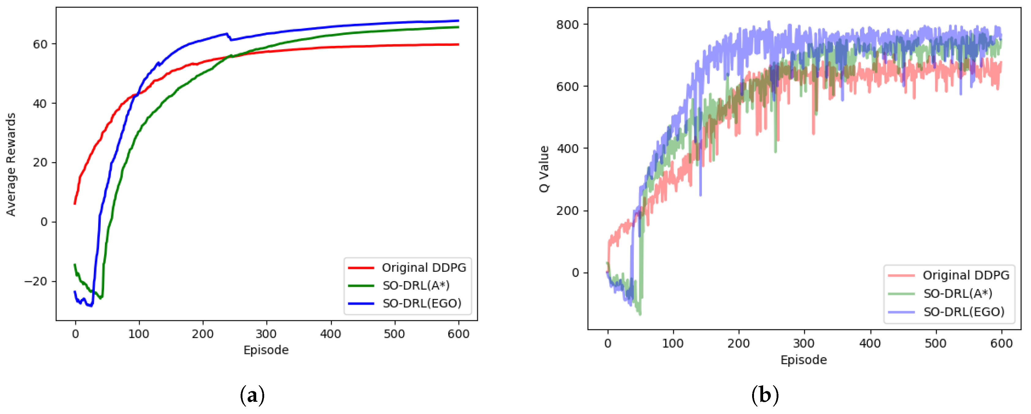
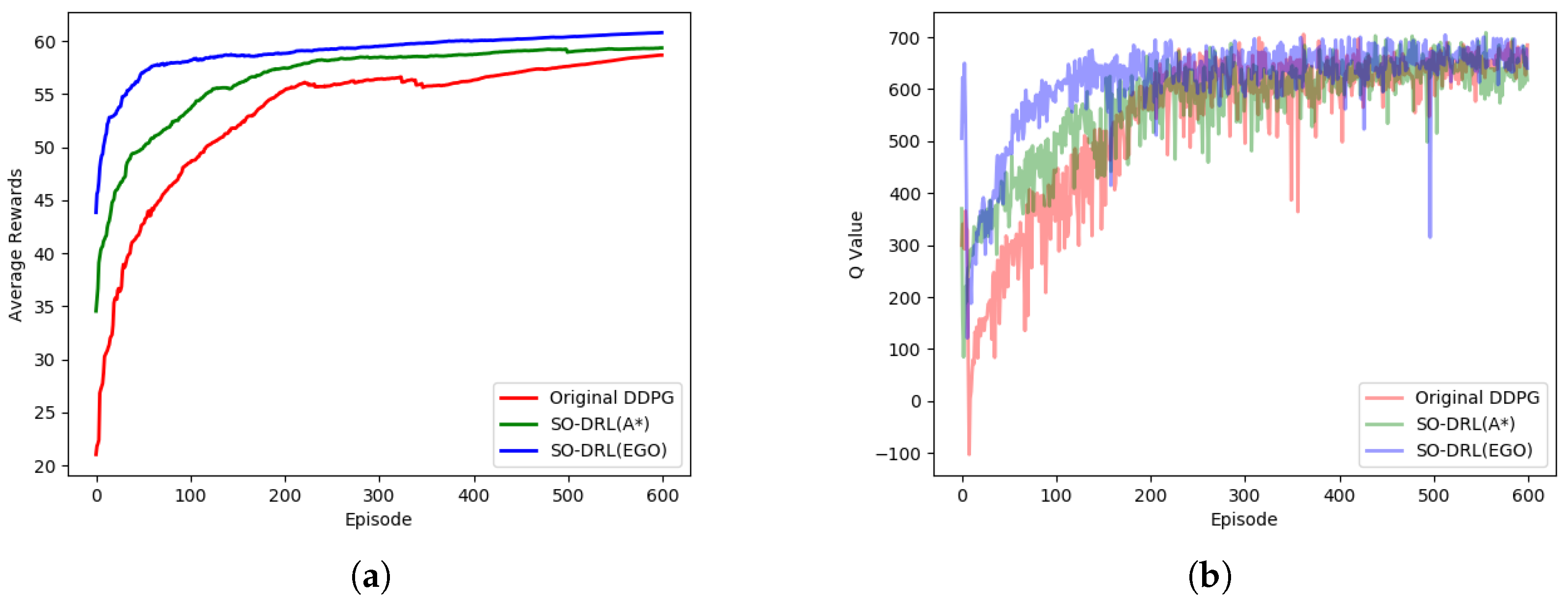
The average reward function and the average Q value for each episode of the first stage are shown in Figure 8. It can be seen that SO-DRL had a negative reward at the beginning of training and some downward floating. This is because there were already some positive and negative rewards of experience in the early stage of training, and the SO-DRL network needed to integrate with the experience and did not achieve good rewards at the early stage. However, as the training progressed, SO-DRL converged relatively faster, especially SO-DRL with EGO-Planner optimization, which was ahead of the original DDPG at 100 episodes, and SO-DRL with A* algorithm optimization, which was ahead of the original DDPG by about 220 episodes. From the performance of the final convergence, the rewards of SO-DRL reached more than 60, while the original DDPG could not break 60, and there was an obvious gap between the two in terms of rewards.

As can be seen from the Q values, it is the uneven sample distribution at the beginning that caused the quantifiers to not be very good at the beginning, but after about 50 episodes, the Q values of SO-DRL were able to exceed the original DDPG. SO-DRL with EGO-Planner optimization converges in less than 200 episodes. Although SO-DRL with A* algorithm optimization converged slightly later than the original DDPG method, SO-DRL eventually converged to a higher Q value than the original DDPG. It can be seen that the overall performance effect of SO-DRL with EGO-Planner optimization was better than SO-DRL with A* algorithm optimization than the original DDPG.

The average reward function and the average Q value for each episode of the second stage are shown in Figure 9. As can be seen by the reward, at the beginning of the second stage, all three methods had certain initial values, and the SO-DRL with EGO-Planner optimization was better than the SO-DRL with A* algorithm optimization than the original DDPG in terms of initial value level, convergence speed, and convergence final value, and the trend and gap of the three curves are obvious. As for the Q values, we can see that the Q values produced some unstable jitter at the beginning due to the new environment, but in the subsequent training process, the advantage of SO-DRL was obvious, indicating that SO-DRL can cope better in longer distances and denser environments.

A comparison of the three strategies shows that search-based optimization had a huge advantage in the learning convergence speed and convergence final value, and it coped better with complex and sparse reward environments.

4.4. Testing Evaluation

We tested the methods in an environment different from the training environment. The test environment contained abundant elements, including columns, square columns, walls, etc. The test scenario was a long corridor (in Figure 10), where the agent needed to go from one end to the other and for more than 20 m.

We tested the success rates of three comparison methods in the test environment. The final weights of the three policies in training were tested 1000 times for the path planning process. The success rate table is in

Table 2. The success rate of the three methods tested in different scenarios.

Method	Success Rate	Episode	Time Consuming
Original DDPG	27.49%	1000	89 min
SO-DRL(A*)	87.23%	1000	84 min
SO-DRL(EGO)	96.64%	1000	83 min

.

It can be seen that the success rate of the original DDPG algorithm was only 27.49%, and its obstacle avoidance ability in such a long-distance environment with dense obstacles was limited. SO-DRL with EGO-Planner optimization is better than SO-DRL with A* algorithm optimization and both SO-DRL methods have excellent path planning and obstacle avoidance effects. It can be seen that SO-DRL outperformed the other two frameworks in generalization performance in different environments.

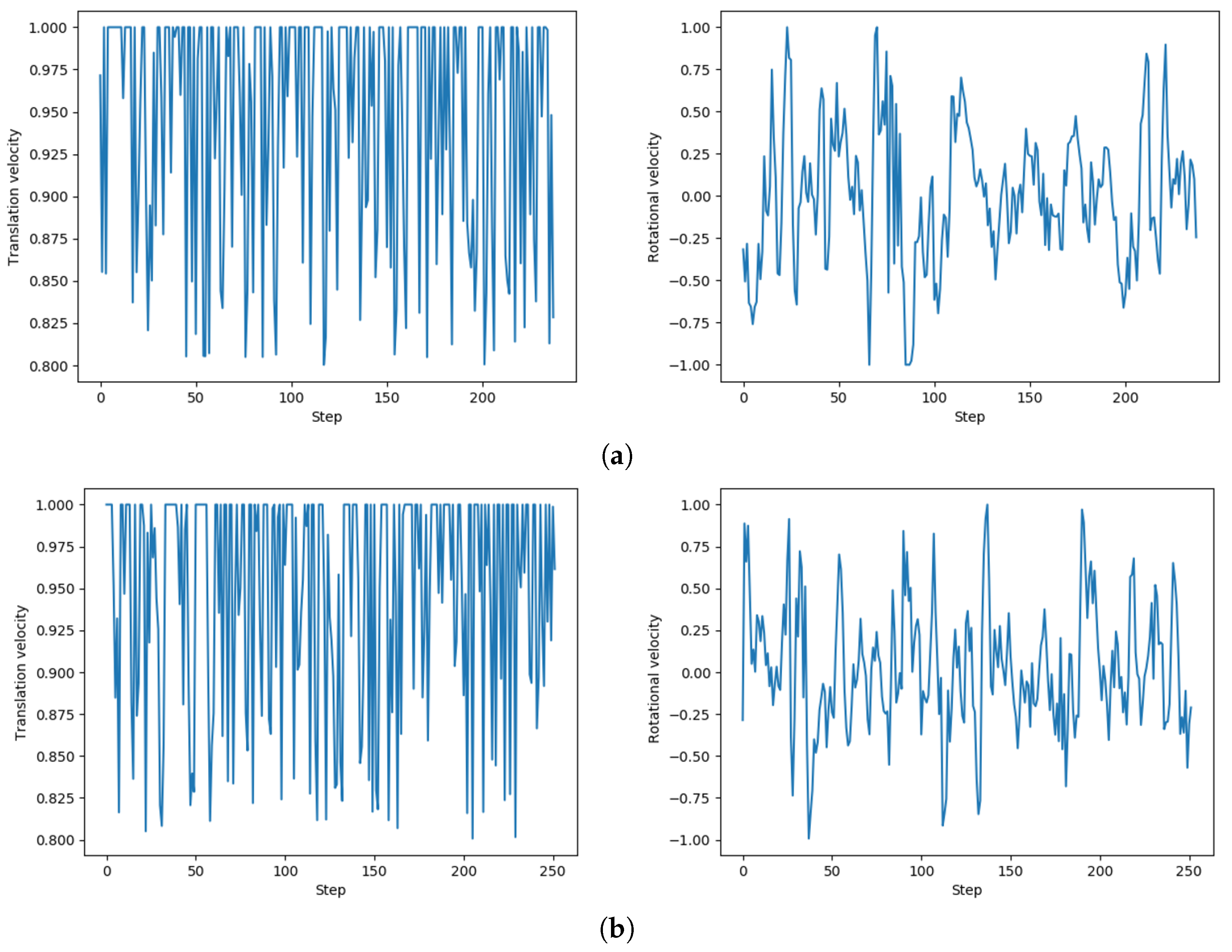
We randomly selected four sets of velocity in the test to demonstrate the control process of our method on the agent in Figure 11.

5. Real World Experiment

The SO-DRL was well validated in a simulation scenario where the training weights were obtained, and the weights were then deployed in a real air–ground unmanned system with no adjustments. We conducted real UGV and UAV path planning and obstacle avoidance experiments in the real world. Experiments were performed using a customized air–ground unmanned system. This section introduces our platform and validates the SO-DRL on a real hardware system.

In the real-world experiment, the construction of the hardware for the air–ground unmanned system was completed. The experiments focused on two aspects. On the one hand, the real-world experiments verified the feasibility of SO-DRL to complete obstacle avoidance and reach the destination in the real world. On the other hand, SO-DRL was able to complete the task in the real world without parameter modification, and the end-to-end algorithm could only be implemented in the real world with weights trained on the computer.

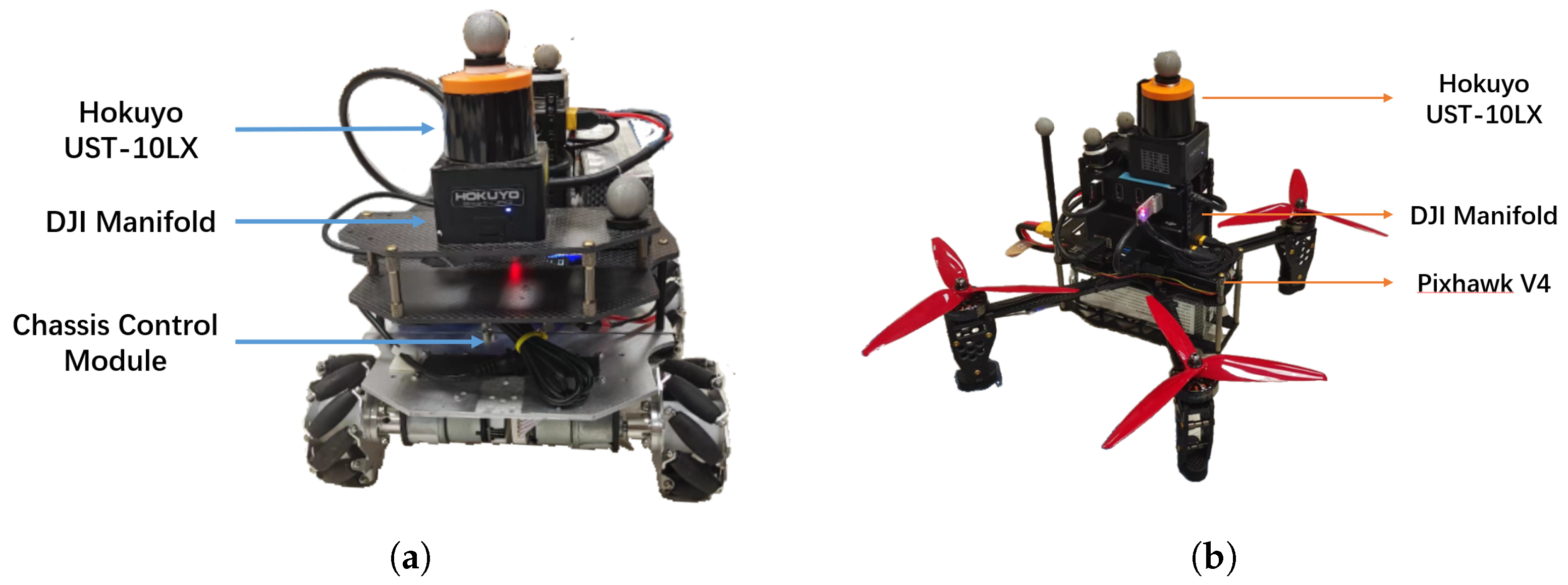
We designed a UGV and a UAV for SO-DRL for the flight experiments (in Figure 12). The UGV (in Figure 12a) was built equipped with McNamee wheels. The UAV (in Figure 12b) consisted of a flight controller Pixhawk V4 on a custom carbon fiber board with a 410 mm diagonal wheelbase. Both the UGV and the UAV mounted DJI Manifold 2-C on-board computer and used a Hokuyo UST-10LX laser scanning survey with 270 degrees for sensing.

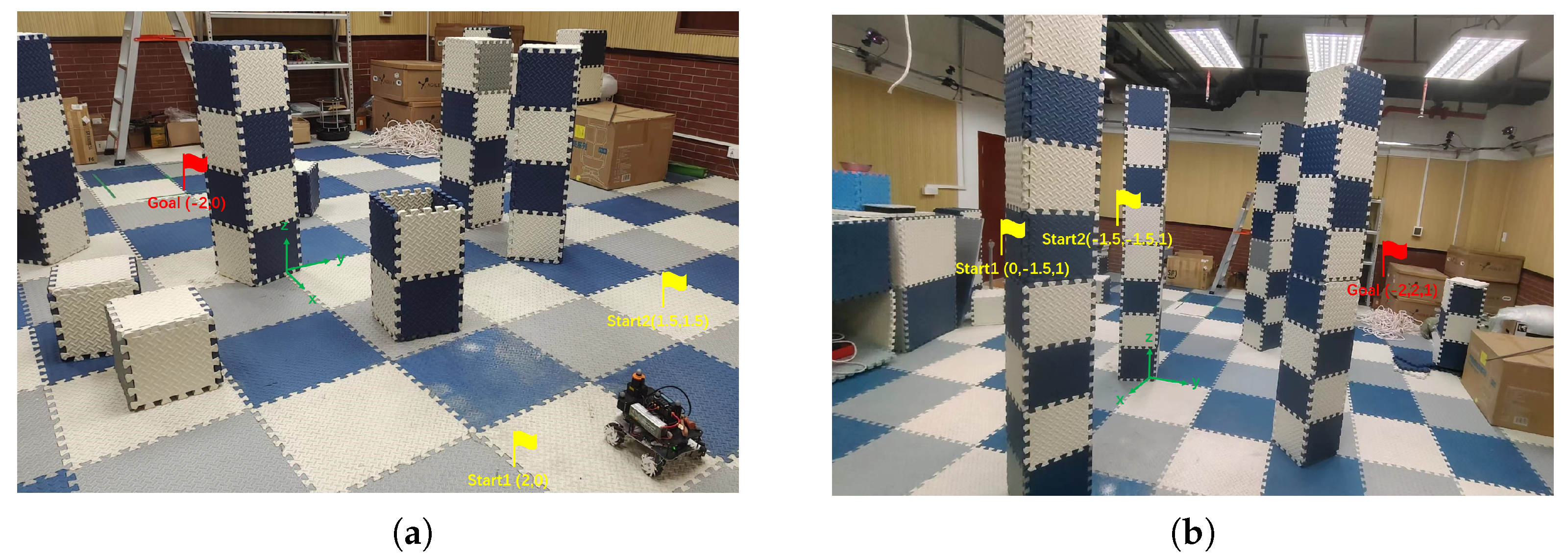
We conducted obstacle avoidance experiments indoors, as shown in Figure 13. The scene was an indoor environment of 4 m × 4 m, and the Vicon indoor positioning system was deployed. Obstacles could be set arbitrarily in the scene. Our experiments had excellent safety and we could choose between manual or automatic mode using a one-to-one pairing remote control. In automatic mode, the controller received a signal from Manifold and used the DRL algorithm for guiding and avoiding obstacles, which made the UGV/UAV fully autonomous. In any case, the manual mode enjoyed the highest control priority ensuring that the entire experiment could be carried out safely.

The experimental environment of UGV is shown in Figure 13a: UGV experiments with the weights trained by A* optimized SO-DRL. The two experiments of the UGV were from the start point (2, 0) to the goal point (−2, 0) and from the start point (1.5, 1.5) to the goal point (−2, 0). The experimental environment of UAV is shown in Figure 13b. UAV is using the weights trained by EGO-Planner optimized SO-DRL. The two experiments of the UAV were from (0,−1.5, 1) to (−2, 2, 1) and from (−1.5, −1.5, 1) to (−2, 2, 1). The results show that SO-DRL was able to act with the laser perception only during the driving process to reach the goal point from the start point while avoiding collision with obstacles.

6. Conclusions and Future Work

In this paper, we proposed an end-to-end deep reinforcement learning framework incorporating search-based approaches for air–ground unmanned system navigation named SO-DRL. Compared to traditional methods, instead of using a map building and planning process, SO-DRL used reinforcement learning to solve the path planning obstacle avoidance problem end-to-end in an unknown environment. In addition to reinforcement learning, SO-DRL adopted the advantage of search-based algorithms. Compared to general reinforcement learning, it had the benefit of quick convergence and superior early realization for target action. Specifically, SO-DRL used the search-based approach and employed prioritized experience replaying, with experiments using a two-stage training process. Experimentally, SO-DRL could improve the training speed and made the training effect reach the expectation well. SO-DRL had an obvious effect improvement over the original DDPG and had a different performance effect under different search-based algorithm optimization, which could effectively solve the path planning problem. SO-DRL worked on real UGV/UAV in the air–ground unmanned system without any parameter adjustment, which has practical implications for real systems.

This paper is an exploration of the intelligence of unmanned systems, but the work in this paper falls short. In our next study, we will use more different algorithms to verify the selection of the algorithm (including more search-based algorithms and reinforcement learning algorithms) and test the adaptation of SO-DRL in different scenarios. We will improve SO-DRL and make it a more sophisticated algorithm. In future work, we intend to incorporate 3D radar, depth maps, and other 3D sensing data to enable path planning and obstacle avoidance in the 3D environment for the UAV. Additionally, we will expand towards increasing the cluster work of UGVs and UAVs and the synergy of both.