Exploring the Relative Importance and Interactive Impacts of Explanatory Variables of the Built Environment on Ride-Hailing Ridership by Using the Optimal Parameter-Based Geographical Detector (OPGD) Model

Abstract

The impact of the built environment on the ridership of ride-hailing results depends on the spatial grid scale. The existing research on the demand model of ride-hailing ignores the modifiable areal unit problem (MAUP). Taking Chengdu as an example, and taking the density of pick-ups and drop-offs as dependent variables, 12 explanatory variables were selected as independent variables according to the “5D” built environment theory. The nugget–sill ratio (NSR) method and optimal parameter-based geographical detector (OPGD) model were used to determine the optimal grid scale for the aggregation of the built environment variables and the ridership of ride-hailing. Based on the optimal grid scale, the optimal data discretization method of the explanatory variables was determined by comparing the results of the geographic detector under different discretization methods (such as the natural break method, k-means clustering method, equidistant method, and quantile method); we utilized the geographic detector model to explore the relative importance and the interactive impacts of the explanatory variables on the ridership of ride-hailing under the optimal grid scale and optimal data discretization method. The results indicated that: (1) the suggested grid scale for the aggregation of the built environment and ride-hailing ridership in Chengdu is 1100 m; (2) the optimal data discretization method is the quantile method; (3) the floor area ratio (FAR), distance from the nearest subway station, and residential POI (point of interest) density resulted in a relatively high importance of the explanatory variable that affects the ridership of ride-hailing; and (4) the interactions of the diversity index of mixed land use ∩ FAR, distance to the nearest subway station ∩ FAR, transportation POI density ∩ FAR, and distance to the central business district (CBD) ∩ FAR made a higher contribution to ride-hailing ridership than the single-factor effect of FAR, which had the highest contribution compared with the other explanatory variables. The proposed grid scale can provide the basis for the partitioning management and scheduling optimization of ride-hailing. In the process of adjusting the ride-hailing demand, the ranking results of the importance and interaction of the built-environment explanatory variables offer valuable references for formulating the priority renewal order and proposing a scientific combination scheme of the built-environment factors.

1. Introduction

By relying on the technological development of the “Internet+”, ride-hailing has become an important part of the modern public transport system [1]. The emergence of Baidu, Gaode, Didi, Uber, and many other ride-hailing software products has brought great convenience to people’s lives. In some American cities, compared with private cars, ride-hailing is conducive to reducing traffic congestion [2] and environmental pollution caused by exhaust emissions, which is of great significance for promoting sustainable development and mitigating traffic congestion [3]. However, it also brings negative impacts such as traffic congestion and low travel efficiency in some cities, such as Manhattan District in New York [4]. Understanding the impact mechanism of the built environment on ride-hailing ridership can provide guidance for ride-hailing management and land use planning.

The factors that affect the ridership of ride-hailing are complex [5]. Some scholars have studied the issue from different perspectives, including the impact of public transport, walking and cycling [6], user characteristics [7], the service attitude of ride-hailing [8], availability [9], etc., on the ridership of ride-hailing. Some scholars have begun to pay attention to the impact of built-environment variables such as transportation, land use, and urban design on ride-hailing travel [10]. Based on the “3D” dimension proposed by Handy [11], namely density, diversity, and design, Kahn added two categories, namely distance to transit and destination accessibility, and proposed a “5D” theory (density, diversity, design, distance to transit, and destination accessibility) [12]. “Density” is measured as the variable of interest per unit of area; “diversity” measures pertain to the number of different land uses in a given area and the degree to which they are represented in land area, floor area, or employment; “design” includes street network characteristics within an area; “distance to transit” is usually measured as an average of the shortest street routes from a residence or workplace in an area to the nearest rail transit station or bus stop; and “destination accessibility” measures the ease of access to trip attractions. The existing research mainly selects explanatory variables based on the “3D” built environment theory. Gao et al. selected explanatory variables from accessibility, land use, population distribution, and facilities [13]; Hui et al. selected explanatory variables from traffic facilities and land use [14]; and Wang et al. selected explanatory variables based on the “5D” built-environment theory from four aspects: density, diversity, urban design, and traffic distance. In addition, a housing price variable was added [15], but the destination accessibility variables were not considered as influencing factors. However, few studies have considered the impact of the explanatory variables of the “5D” dimension of the built environment on the ridership of ride-hailing.

The scale difference for the data aggregation of ride-hailing ridership and built-environment variables will affect the analysis results. The spatial object exists only after a set of real collected data is aggregated to spatial units [16]. The first step of many spatial research problems is to divide the aggregation area [17]. Many types of big geo-data are used for urban studies where the size of the analysis unit determines the amount of data to be included and affects the value of each unit, and it is more important to look into the scale effect of big geo-data [18]. Therefore, the size (i.e., scale) and shape of the aggregation area will affect the analysis results. Openshaw describes this phenomenon as a modifiable area unit problem, which refers to the problem that the analysis results vary with the definition of the basic area units [19]. The MAUP problem has two aspects. One is the scale effect, that is, different area unit sizes; the other is the zoning effect, that is, area elements with different shapes, such as a square grid [20], traffic analysis zone [21,22,23], Voronoi diagram [14,21,22,23,24,25], etc. Previous work selected a spatial scale. For example, Wang et al. selected a 200 × 200 m square grid as the basic unit to study the impact of the built environment on ride-hailing [15]; Liu et al. selected a 500 × 500 m square grid as the basic unit of land use classification in Shanghai [26]; and Pei et al. selected a 200 × 200 m square grid as the basic unit of land use classification in Singapore [27]. The methods for determining the optimal scale include the nugget–sill ratio (NSR) [18], the optimal parameter-based geographical detector (OPGD) [28], and comparison of the coefficient of determination R² values from multiple regressions [29] at different scales. The NSR determines the best scale by comparing the ratio of intra-unit variance and inter-unit variance, because variance represents how much information is lost in the process of aggregation [16], and the NSR only considers dependent variables [18]; the OPGD compares the 90% quantiles of the q value results of the geographical detectors at different scales and selects the scale corresponding to the maximum 90% quantile of the q value of all explanatory variables as the best scale, and independent and dependent variables are also considered [28]. The existing research on ride-hailing mostly uses grids as area units [15], and there are few studies on the optimal scale of impact for the built environment on the ridership of ride-hailing.

This paper mainly summarizes related studies about ride-hailing from the aspects of variable selection, the size of the analysis unit, and modeling methods, as shown in

Table 1. Summary of relevant research on ride-hailing.

Author	Study Area	Dependent Variable(s)	Analysis Method(s)	Space Unit	Independent Variable(s)	Main Conclusion
Bi, H., et al. [14]	Chengdu	Online car-hailing drop-off ridership	GWR	Voronoi cells	Workplaces, education services, leisure services, medical services, residential buildings, food services, shopping services, parking lots, and road density.	The places with high densities of road networks or parking lots have a higher likelihood of online car-hailing trip generation.
Wang, S. C, et al. [15]	Chengdu	Online car-hailing pick-ups and drop-offs	OLS and GWR	200 × 200 m grid cell	Population density, local road density, FAR, housing prices, mixed land use entropy, sport and entertainment facilities, restaurant facilities, and retail facilities.	The association between spatial characteristics and ride-hailing trips in Chengdu and the influence of the built environment on ride-hailing trips at different times was examined.
Du, M. Y. et al. [30]	Haikou	The spatiotemporal variation in high-efficiency ride-hailing orders (HROs) and common ride-hailing orders for ride-hailing services	OLS and GWR	1000 × 1000 m grid cell	Built environment variables and POI diversity.	Factors including road density, average travel time rate, companies and enterprises, and transportation facilities have significant impacts on HROs and common ride-hailing orders (CROs) for most periods.
Zhuo Y, et al [31]	Washington D.C.	Taxi pick-up and drop-off trips	OLS	Traffic analysis zones (TAZs)	Number of bus stops, metro stations within a half-mile buffer, existence of an airport, population and residential density, average block size, entropy of employment, industrial employment density, retail employment density, office employment density, and other employment density.	Taxi demand patterns in the Washington D.C. metropolitan area were assessed through traditional methods.
Li, T., et al. [32]	The northeast of Chengdu	Car-hailing pick-ups	OLS and GWR	500 × 500 m grid cell	Bus station POI, shopping service POI, corporate business POI, residential district POI, catering service POI, recreation and entertainment POI, and mixed land use.	Recreation and entertainment POI and the residential district POI are the most influential factors on night online car-hailing travel.
Zhang, X. X. et al. [33]	New York City	Pick-ups at taxi zones in a certain month	GTWR	263 taxi zones	Fourteen influencing factors from four groups, including weather, land use, socioeconomic factors, and transportation, were selected as independent variables.	Transportation network companies (TNCs) have become more convenient for passengers in snowy weather, while a traditional taxi (TT) is more concentrated at the locations close to public transportation. The socioeconomic properties are the most important factors that cause the difference in spatiotemporal patterns.
Wang, S., et al. [34]	Chengdu	Online car-hailing pick-ups and drop-offs	MGWR and SDM	500 × 500 m grid cell	Bus station, residential district, catering services, shopping services, corporate businesses, sports and leisure services, science zones, public facilities, finance and insurance services, education and culture, life services, medical and health, government and administration, accommodation services, mixed land use, people density, distance to central business district (CBD), orientation order, and road network density.	Catering services, corporate businesses, and orientation order have significant positive spillover effects, while the spillover effects of sports and leisure services and mixed land use are negative. The bus stations, residential districts, catering services, shopping services, corporate businesses, mixed land use, life services, and orientation order have significant spatial heterogeneity.
Nair, G. S. et al. [35]	Burnet, Bastrop, Caldwell, Hays, Travis, and Williamson	Deadheading trips	Nonlinear-in-parameter multinomial logit	2102 traffic analysis zones	Built environment, employment opportunities, and socio-demographic characteristics.	The model results shed light on the characteristics of deadheading trips at different locations and at different time periods in a day.
Zhao, G. W., et al. [36]	Chengdu	Online car-hailing pick-ups and drop-offs	Stepwise regression selection and three spatial regression models	500 m grid to 5000 m grid	Population density; mixed land use; road density; bus stop density; catering facility density; scenic spot density; public service facility density; company density; shopping facility density; transportation facility density; financial facility density; educational, scientific, and cultural facility density; residential district density; living service facility density; sports and leisure facility density; medical service facility density; government agency density; and accommodation service facility density.	The effects of population density and road density are always positive from the 500 m grid to the 3000 m grid. As the analysis scale increases, the effect of proximity to public transportation shifts from inhibition to facilitation, while the positive effect of mixed land use becomes stronger. The land-use type has both positive and negative effects and shows different characteristics at different scales.
Sabouri, Sadegh, et al. [37]	24 regions across the USA	Natural log of trips between two census block groups; average trip duration between census block groups	Multilevel modeling (MLM)	24 regions across the USA	A total of 39 independent variables.	The Uber demand is positively correlated with total population and employment, activity density, land use mix or entropy, and transit stop density of a census block group. In contrast, the Uber demand is negatively correlated with intersection density and destination accessibility (both by auto and transit) variables.
Tu, Meiting, et al. [38]	Chengdu	The ride-splitting ratio of each OD pair	Gradient-boosting decision tree	162 census tracts based on the administrative boundaries	The built environment at the origin locations, the built environment at the destination locations, demographic factors, and travel time.	Distance to city center, land use diversity, and road density are the key influencing factors of the ride-splitting ratio.
Müller, et al. [39]	Berlin	Booking data of free-floating carsharing	Negative binomial model	Cells based on the polling districts and the census data grid	Census data, election behavior, density of points of interest (POIs), and centrality.	Built-environment features, including location, street design, parking supply, and neighborhood centrality, are major factors that affect the carsharing demand.

. In terms of modeling methods, OLS [30,31], GWR [14,15,30,32], GTWR [33], MGWR [25,34], a nonlinear regression model [35], and other models [36,37,38,39] have often been used in the research investigating built-environment impacts on the ridership of ride-hailing, and the global impact or local spatial heterogeneity of each built-environment variable on ride-hailing is analyzed separately. The geographical detector can detect the influence of a single variable and the interaction of variables, and eliminate the influence of the multicollinearity of variables [40]. The geographical detector model has been widely used in research in various fields, such as health risk assessments [40,41,42,43,44,45,46], crime prediction [47,48], land health assessments [49,50], carbon emission influencing factors [51,52], etc. To the best of our knowledge, the geographical detector model has not been used in the impact of the built environment on the ridership of ride-hailing.

These studies have shown that the built environment has an important impact on the ridership of ride-hailing. However, few studies have considered the impact of the modifiable areal unit problem (MAUP) on the ride-hailing analysis results. In addition, existing studies have not analyzed the interaction effects from built-environment factors on ride-hailing ridership. To fill the above gaps, this study utilized the nugget–sill ratio (NSR) [18] method and the optimal parameter-based geographical detector (OPGD) [28] model to explore the relative importance and interactive impacts of the explanatory variables of the built environment on ride-hailing ridership, mainly solving the following four questions: (1) What is the optimal grid scale for the aggregation of the built environment and the ridership of ride-hailing? (2) What is the optimal data discretization method of the explanatory variables for the geographic detector model? (3) What is the ranking of the impact importance of the built-environment variables? (4) How effective is the interaction of variable combinations? After considering the MAUP problem to determine the optimal grid scale, the mechanism of the influence of built environment factors on the ridership will improve the reliability of the results. The importance degree of the built-environment variables and their interaction results are more useful for proposing a scientific planning scheme for a built-environment renovation.

2. Study Area and Data Sources

2.1. Overview of the Study Area

Located in the middle of the Sichuan province, Chengdu is the economic center and transportation hub of southwest China. The area within the Third Ring Road of Chengdu was selected as the study area (Figure 1), which covers an area of about 200 square kilometers.

2.2. Data Sources

Through the “GAIA Open Dataset of Didi Chuxing” (https://gaia.didichuxing.com, accessed on 10 October 2019), we selected data from five working days (7 November 2016 to 11 November 2016) for this research. The field information contained in the data is shown in

Table 2. Driving trajectory data of ride-hailing.

Field Name	Field Type	Example	Field Description
Order ID	String	fb2571ff396f07fc5f57aca2c1f9ef49	Order No.
Driver ID	String	oyEiito1mvarq3gwqpzEjmomatuimy	Driver’s ID
Start Time	String	7 November 2016 12:36	Pick-up time
End Time	String	7 November 2016 12:53	Drop-off time
Minute	Short integer	17	Order duration of ride-hailing
Lon	Float	103.9915468	Longitude, GCJ-02 coordinate system
Lat	Float	30.6471488	Latitude, GCJ-02 coordinate system

. The average sampling interval was about 3 s, with a total of 1,145,146 entries; through Python web crawler, we obtained point of interest (POI) data for various facilities in Chengdu, with 13 categories and 2,357,377 data points in total, including the names, types, coordinates, and other information of the POIs. The population distribution data of Chengdu were derived from the WorldPop website, which is a grid map with a resolution of 100 × 100 m.

3. Methods

3.1. Dependent Variables and Explanatory Variables

The regular grid was selected as the spatial unit, and the spatial grid scale represented the spatial aggregation range, as shown in Figure 2. The aggregate results of the explanatory variables of the built environment and ride-hailing demand under different scale grids were different.

The dependent variable in this paper was the density of pick-ups and drop-offs of ride-hailing during the morning and evening peak hours. Based on the “5D” dimension of the built environment, 12 variables (

Table 3. Built-environment explanatory variables.

“5D” Built-Environment Dimension	Explanatory Variable	Unit
Density	Population density	Person/km2
	FAR
	Commercial POI density	Quantity/km2
	Public service POI density	Quantity/km2
	Residential POI density	Quantity/km2
	Scenic spot POI density	Quantity/km2
	Transportation POI density	Quantity/km2
	Building density	%
Diversity	Diversity index of mixed land use
Destination accessibility	Distance to CBD	km
Distance to transit	Distance to the nearest subway station	km
Design	Road network density	km/km2

) were selected to establish the influencing factor system of the built environment. The population density, FAR, commercial POI density, public service POI density, residential POI density, scenic spot POI density, transportation POI density, and building density were selected as eight indicators of the density dimension. Commercial POIs consist of shopping centers, supermarkets, and convenience stores. Transportation POIs consist of bus stops, subway stations, railway stations, airports, and parking lots. Public service POIs consist of emergency shelters, public restrooms, and newsstands. The diversity factor represents the distribution of different types of land, the diversity index of mixed land use was selected as the measurement index, and the Shannon–Weiner diversity index was used for the calculation [53]. The distance to the CBD was selected as the measurement index of the destination accessibility dimension. The road network density was selected as the measurement index of the design dimension, which can reflect the connectivity of urban roads to a certain extent, and the distance from the nearest subway station was selected as the measurement index of the distance-to-transit factor.

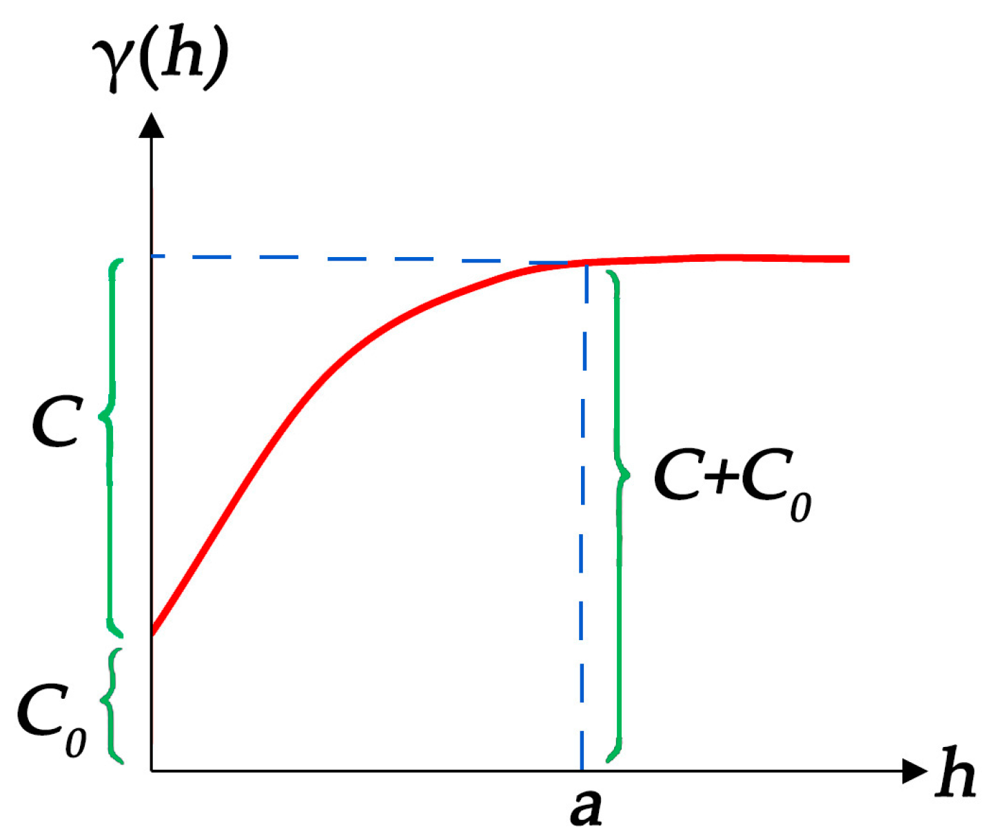
3.2. Determination of the Optimal Scale of Spatial Grid

The semi-variogram, as shown in Equation (1), is an important tool for analyzing the spatial heterogeneity of regionalized variables [18], and can be used to determine the optimal spatial grid scale for the study of the influencing factors on the ridership of ride-hailing in Chengdu. Assuming that the regionalized variables satisfy the second-order stationary and intrinsic assumptions, the semi-variogram formula is as follows [54]:

$$\mathsf{\gamma }(h) \frac{1}{2N\left(h\right)}{{\displaystyle \sum }}_{i=1}^{N\left(h\right)}{\left[Z\left(x_i\right)-Z\left(x_i+h\right)\right]}^2$$

(1)

where γ(h) is the semi-variation value for the ridership of ride-hailing, N is the number of pairs of points, x_i is the i-th pair of points, Z is the ridership of ride-hailing, x is the spatial location of ride-hailing pick-ups or drop-offs, Z(x) is the ridership of ride-hailing at point x, h is the spatial lag distance, and x + h is another point with h distance from point x.

The discrete variation value of the ride-hailing demand was obtained through the formula, but it could not reflect the spatial variation characteristics of the ride-hailing demand at different spatial lag distances. Therefore, it was necessary to fit the discrete variation values through the fitting model of the commonly used semi-variogram. The commonly used models include the Gaussian model [55,56], the exponential model [57,58], the spherical model [59], and the rational quadratic model [60]. The suitable models were selected according to the fitting determination coefficient (R²) and residual sum of squares (RSS) of different models.

Figure 3 shows the semi-variogram fitting curve of the selected Gaussian model. C₀ is the nugget variance, which represents the spatial variation of the ridership of ride-hailing affected by random factors. It can be used to quantify the intra-unit variation in the ridership of ride-hailing gathered at different scales. There are two reasons for this: on the one hand, it is the internal variation of the regionalized variable Z(x) when it is smaller than the sampling scale h; on the other hand, it is the error during data collection [61]. C is the partial base value and the increment of the semi-variogram value that remains stable, indicating the variation caused by the spatial structure of ridership of ride-hailing; C₀ + C is the base value, representing the total spatial variation of the ridership of ride-hailing; and a is the range, that is, the sampling distance corresponding to when the semi-variogram reaches a stable value, indicating the influence range of the regionalized variable [29,62].

The relationship between the spatial lag distance and the grid scale can be divided into three categories: the spatial lag distance is greater than the grid scale, the spatial lag distance is equal to the grid scale, and the spatial lag distance is less than the grid scale, which respectively correspond to inter-grid variations, adjacent grid variations, and intra-grid variations. In order to compare the aggregation effect under different scales, the block-to-base ratio C₀/(C₀ + C) was defined as the NSR [18]. The NSR is the ratio of intra-grid variance to inter-grid variance. The smaller the NSR, the smaller the ratio of intra-grid variance to inter-grid variance. It proves that the stronger the spatial dependence, the less information loss and the better the scale in the aggregation process [29,63,64].

3.3. Influencing Factors and Interaction of Ride-Hailing Demand

The geographic detector is a statistical method for detecting spatial heterogeneity and its driving factors, including a factor detector, an interaction detector, a risk detector, and an ecological detector [40,65]. The factor detector and interactive detector were used to study the influence of built-environment variables on the ridership of ride-hailing. The influence of built-environment variables on the ridership of ride-hailing was measured by the q value. The q value indicates the factor’s explanatory power on the spatial distribution of the dependent variable [40]. The larger the q value, the stronger the contribution of the factors to the spatial distribution of the ridership of ride-hailing. The q value of the explanatory variable m was computed by:

$$q_m=1-\frac{1}{N_m{\sigma }_m^2}{\displaystyle \sum }_{h=1}^L{N}_{m,h}{\sigma }_{m,h}^2$$

(2)

where L is the number of sub-regions of variable m; N_m,h is the number of units in the h-th (h = 1, …, L) sub-region of variable m; ${\sigma }_{m,h}^2$ is the variance in the h-th (h = 1, …, L) sub-region of variable m; N_m is the number of units within the whole study area; and ${\sigma }_m^2$ is the variance in the independent variable m for the whole study area.

The interaction detector can identify whether or not the interaction between different influencing factors of the built environment increases or decreases, and how to increase or decrease the impact on the ridership of ride-hailing. There are five kinds of interaction results, as shown in

Table 4. Interactions between two explanatory variables and their interactive impacts.

Geographical Interaction Relationship	Interaction
qm∩n < min(qm, qn)	Nonlinear-weakened: Impacts of single variables are nonlinearly weakened by the interaction of two variables.
min(qm, qn) ≤ qm∩n ≤ max(qm, qn)	Uni-variable weakened: Impacts of single variables are uni-variably weakened by the interaction.
max(qm, qn) < qm∩n < (qm + qn)	Bi-variable enhanced: Impact of single variables are bi-variably enhanced by the interaction.
qm∩n = (qm + qn)	Independent: Impacts of variables are independent.
qm∩n > (qm + qn)	Nonlinear-enhanced: Impacts of variables are nonlinearly enhanced.

Note: q_m is the q value of variable m, q_n is the q value of variable n, and q_m∩n is the q value of the interaction between variables m and n.

, namely nonlinear-weakened, univariable weakened, bi-variable enhanced, independent, and nonlinear-enhanced [40].

4. Results and Discussion

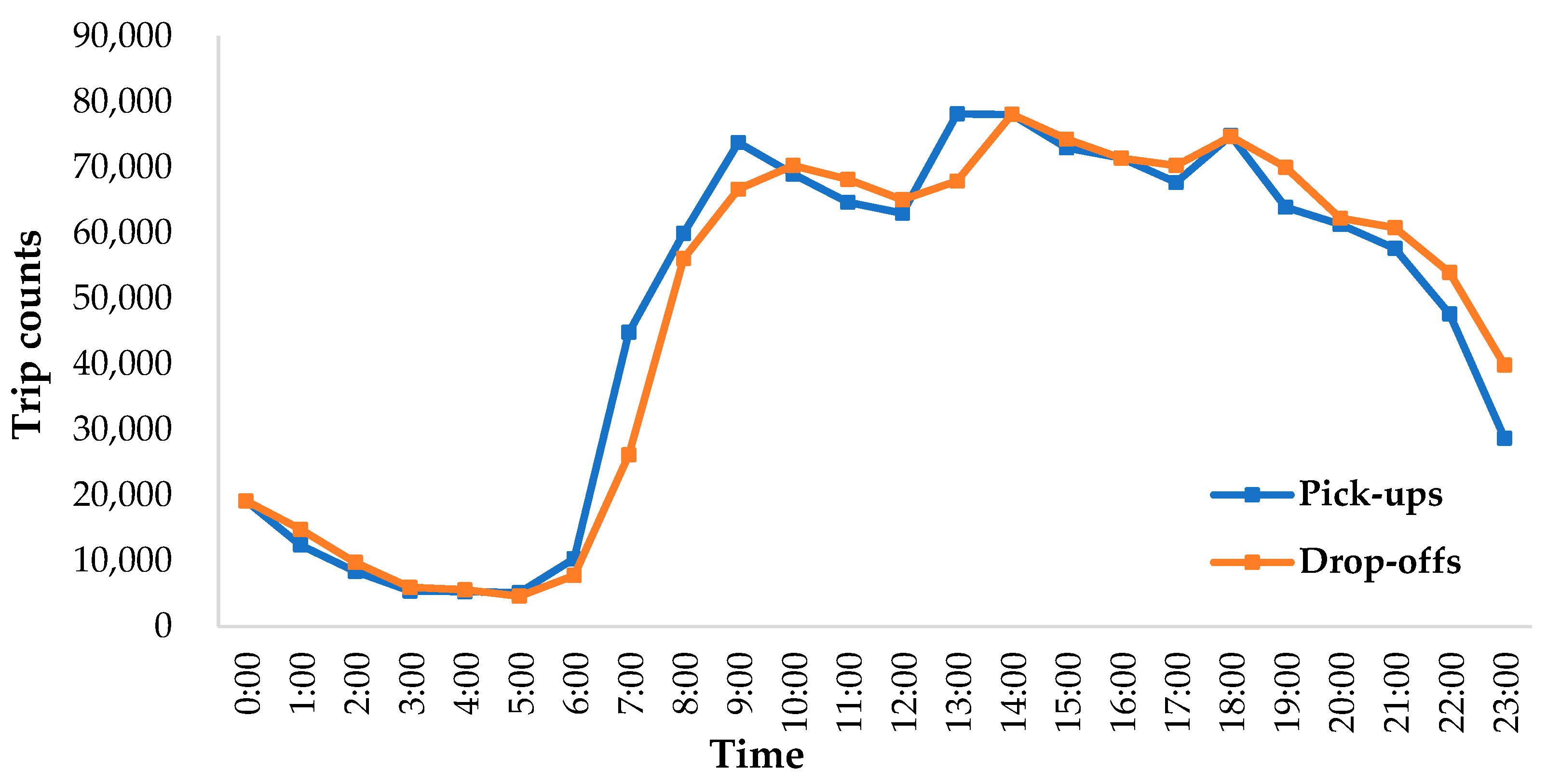
4.1. Spatial and Temporal Characteristics of Ride-Hailing in Chengdu

The sum of the ridership of ride-hailing in Chengdu from 7 November 2016 to 11 November 2016 was calculated by the hour, and the results are shown in Figure 4. Considering that a large number of commuting trips on weekdays were concentrated in the morning and evening peak hours, and the traffic demand and travel efficiency of these two periods were the most widely concerned by travelers and researchers, we chose the pick-ups and drop-offs of ride-hailing during the morning and evening peak hours as the dependent variables. It can be seen from the figure that the morning peak hours and the evening peak hours were, respectively, from 8:00 to 9:00 and from 18:00 to 19:00.

The ridership of ride-hailing on weekdays under a grid size of 1100 m is shown in Figure 5. The ridership of ride-hailing in the morning peak hours was more concentrated than that in the evening peak hours, and the pick-up behavior was mainly concentrated in the First Ring Road. The ridership of ride-hailing in the evening peak hours was relatively scattered, and the pick-up behavior was mainly concentrated within the First Ring Road. The drop-off behavior was mainly concentrated in the business district in the east section of the First Ring Road; a dense area of passengers with drop-off behavior also formed in the north section of the First Ring Road. On the whole, the ridership of ride-hailing in the south section of the Ring Road was less than that in the north section.

4.2. Optimal Scale of Spatial Grid and Optimal Data Discretization Method

4.2.1. Optimal Grid Scale

We used python code [18] to calculate the NSR, and the result is shown in Figure 6. The optimal grid scale of the pick-up ridership in the morning peak hours of working days in Chengdu was 1100 m, the optimal scale of the drop-off ridership in the morning peak hours and the pick-up ridership in the evening peak hours was 900 m, and the optimal scale of the drop-off ridership in the evening peak hours was 1100 m. The first local minimum value should be taken as the best measure for two reasons: first, according to the elbow theory [66], after the elbow point, increasing the number of clusters will produce new clusters that are very close to the existing clusters, and the rate of cost decline will slow down. Secondly, as a choice of people’s travel modes, the research on the influencing factors of ride-hailing should be based on a more detailed scale to better analyze the relationship between the built environment and the ridership of ride-hailing, since an excessive grid scale may obscure some of the spatial heterogeneity of the ridership of ride-hailing.

The results calculated by the OPGD model are shown in Figure 7. During the morning peak hours, the optimal grid scale for studying the impact of the built environment on the pick-up ridership was 1000 m, the optimal grid scale for the morning peak hour and evening peak hour drop-off ridership was 1300 m, and the optimal grid scale for the pick-up ridership in the evening peak hours was 1200 m.

The comparative analysis of the impact of the built-environment explanatory variables on the pick-ups and drop-offs of ride-hailing in the morning and evening peak hours needed to be carried out under a unified grid scale. We suggested taking the average value of these optimal grid scales just mentioned for the next analysis. The suggested grid scale for exploring the impact of the built environment on the ridership of ride-hailing in Chengdu was 1100 m.

4.2.2. Optimal Data Discretization at Optimal Grid Scale

The geographic detector is good at processing type variables, and numerical variables need to be converted into type variables, that is, discretization. Four commonly used data discretization methods were selected: the natural break method, the equal interval method, the quantile method, and the k-means clustering method [67]. The q value of the geographical detector was used as the index to measure the classification method. The results of different discrete methods are shown in

Table 5. The results for the q values of the geographical detector.

Variables	Discretization Method	q Value
		Pick-up Ridership in the Morning Peak Hours	Drop-off Ridership in the Morning Peak Hours	Pick-up Ridership in the Evening Peak Hours	Drop-off Ridership in the Evening Peak Hours
Distance to the nearest subway station	NB	0.13	0.13	0.13	0.11
	EQ	0.08	0.04	0.06	0.07
	QU	0.13	0.17	0.15	0.13
	K	0.13	0.13	0.12	0.11
Road network density	NB	0.12	0.06	0.10	0.10
	EQ	0.07	0.03	0.05	0.06
	QU	0.13	0.07	0.10	0.12
	K	0.13	0.06	0.09	0.12
Population density	NB	0.11	0.07	0.10	0.10
	EQ	0.00	0.00	0.01	0.01
	QU	0.13	0.08	0.12	0.12
	K	0.10	0.07	0.09	0.09
Building density	NB	0.14	0.12	0.11	0.12
	EQ	0.10	0.11	0.11	0.12
	QU	0.15	0.13	0.13	0.14
	K	0.12	0.10	0.11	0.12
Transportation POI density	NB	0.22	0.10	0.17	0.21
	EQ	0.11	0.04	0.08	0.10
	QU	0.19	0.10	0.14	0.17
	K	0.18	0.07	0.12	0.15
Scenic spot POI density	NB	0.15	0.11	0.10	0.13
	EQ	0.09	0.03	0.04	0.03
	QU	0.13	0.12	0.11	0.13
	K	0.18	0.10	0.13	0.13
Residential POI density	NB	0.22	0.18	0.21	0.21
	EQ	0.17	0.04	0.09	0.11
	QU	0.22	0.17	0.21	0.22
	K	0.23	0.15	0.19	0.21
Public service POI density	NB	0.19	0.11	0.13	0.16
	EQ	0.04	0.00	0.02	0.04
	QU	0.17	0.10	0.14	0.16
	K	0.16	0.07	0.10	0.13
Commercial POI density	NB	0.17	0.08	0.11	0.13
	EQ	0.05	0.01	0.01	0.02
	QU	0.14	0.07	0.08	0.10
	K	0.17	0.08	0.10	0.13
Diversity index of mixed land use	NB	0.15	0.08	0.09	0.13
	EQ	0.08	0.02	0.05	0.07
	QU	0.13	0.10	0.09	0.10
	K	0.12	0.05	0.07	0.10
FAR	NB	0.18	0.13	0.16	0.20
	EQ	0.21	0.13	0.19	0.21
	QU	0.23	0.17	0.22	0.24
	K	0.21	0.15	0.19	0.22
Distance to CBD	NB	0.01	0.02	0.00	0.01
	EQ	0.00	0.02	0.00	0.00
	QU	0.01	0.08	0.04	0.03
	K	0.00	0.04	0.01	0.01

Notes: K represents the k-means clustering method; QU stands for the quantile method; EQ stands for the equal interval method; and NB stands for the natural break method.

. The larger the q value, the better the discrete effect [40]. For the pick-up ridership in the morning peak hours, the drop-off ridership in the morning peak hours, the pick-up ridership in the evening peak hours, and the drop-off ridership in the evening peak hours of ride-hailing in Chengdu, among the 12 factors of the built environment, the highest proportion of the maximum q value was obtained using the quantile method, accounting for 50%, 75%, 75%, and 75%, respectively. The quantile method was regarded as the optimal data discretization method, which is different from the conclusions of other studies that the natural break method is the optimal discrete method [13].

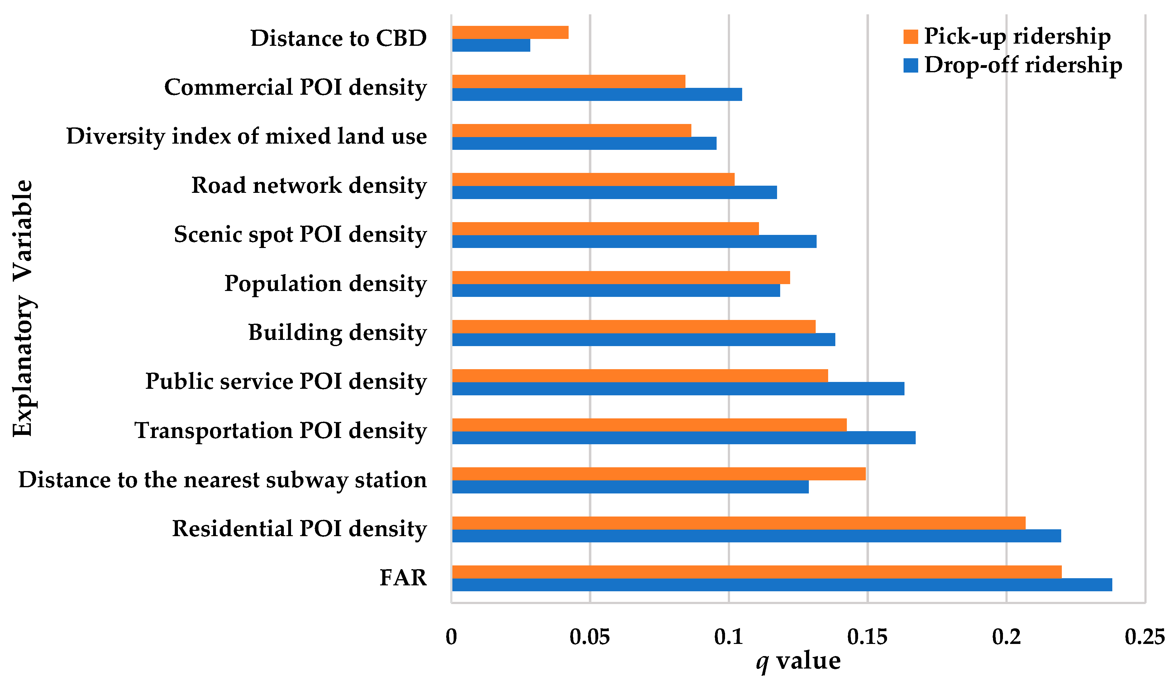
4.3. Factor Detection Results under Optimal Grid Scale and Optimal Discrete Method

The q value indicates the factor’s explanatory power to the spatial distribution of the dependent variable [40]. The larger the q value, the stronger the contribution of factors to the spatial distribution of the ridership of ride-hailing. The factor detection results for morning peak hours and evening peak hours are shown in Figure 8 and Figure 9, respectively. The FAR, residential POI density, and transportation POI density were the major contributors to the pick-up ridership in the morning peak hours, with contributions of 23%, 22%, and 19%, respectively. This may be because residents commute regularly on working days. In the morning, people leave the residential area to work, and the residential area is mostly distributed in clusters. Therefore, the demand conflict of pick-ups in the morning peak hours is mainly concentrated in places with a high FAR and residential POI density, and more ride-hailing vehicles should be allocated to these areas. In addition, as one of the important commuting tools, a ride-hailing vehicle is a substitute for or supplement to public transport [4,68]. During rush hours, the transfer behavior of ride-hailing occurs in areas with a high POI density, such as bus and subway stations. Therefore, ride-hailing companies should pay attention to the allocation of vehicles in such areas during the morning peak hours. The FAR, residential POI density, and distance to the nearest subway station are the major contributors to the drop-off ridership in the morning peak hours, with contributions of 17.4%, 17.2%, and 17.2%, respectively. The reason why the FAR has a relatively high importance for drop-off ridership in the morning peak hours is that most destinations of the commuters in the morning peak hours are CBD areas with a high FAR. Therefore, the transport department should pay attention to the monitoring of traffic conditions in the areas with a high FAR during this period to avoid traffic congestion caused by more of the drop-off behavior of ride-hailing. In addition, temporary stops for ride-hailing vehicles can be located around the subway station to encourage residents to use ride-hailing services in an orderly manner.

The FAR, residential POI density, and distance to the nearest subway station are the major contributors to the pick-up ridership in the evening peak hours, with contributions of 22%, 21%, and 15%, respectively. The distance to the nearest subway station may have had a relatively high importance for the pick-up ridership, because as a reservable travel mode, ride-hailing is a better choice for residents to solve the “last 1 km” problem [4]. The main influencing factors of the pick-up ridership in the evening peak hours were consistent with the ones of the drop-off ridership in the morning peak hours. The possible reason is that the pick-up locations in the evening were mostly the same as the drop-off locations in the morning. The FAR, residential POI density, and transportation POI density were the major contributors to the drop-off ridership in the evening peak hours, with contributions of 24%, 22%, and 17%, respectively. This is mainly because some people return to their places of residence after work, that is, residential areas with a high FAR. Another reason is that the POI of transportation facilities includes airports, railway stations, bus stations, and other transportation facilities. The people who use such facilities as destinations are mainly divided into two categories: one is the staff of such facilities, who use ride-hailing vehicles as commuting tools, and the other is people who meet someone or drop them off at the station, so the stop-and-go mode of ride-hailing is a more suitable choice for them.

In the four cases, the FAR and residential POI density were the major contributors to the ridership of ride-hailing, with the highest q values. The top three variables that were the major contributors to the ridership of ride-hailing drop-offs in the morning peak hours and pick-ups in the evening peak hours, in descending order of importance, were the FAR, the residential POI density, and the distance to the nearest subway station. The top four variables that were the major contributors to the pick-ups in the morning peak hours and the drop-offs in the evening peak hours, in descending order of importance, were the FAR, the residential POI density, the transportation POI density, and the public service POI density. For the same variable, the sizes of the two q values for pick-ups and drop-offs in the morning peak hours were significantly different, while the sizes of the two q values for pick-ups and drop-offs in the evening peak hours were less different. In other words, there were differences in the level of influence importance of the built-environment variables on the pick-ups and drop-offs during the morning peak hours. The possible reason is that ride-hailing destinations are relatively concentrated in some employment-intensive areas during the morning peak hours, while the starting points and destinations of ride-hailing trips during the evening peak hours are scattered.

It is worth noting that the diversity index of mixed land use had less of an effect on the ridership of ride-hailing. This may be because more people tend to travel on foot in these areas [15], and the allocation of vehicles to the area with a higher diversity index of mixed land use should be reduced.

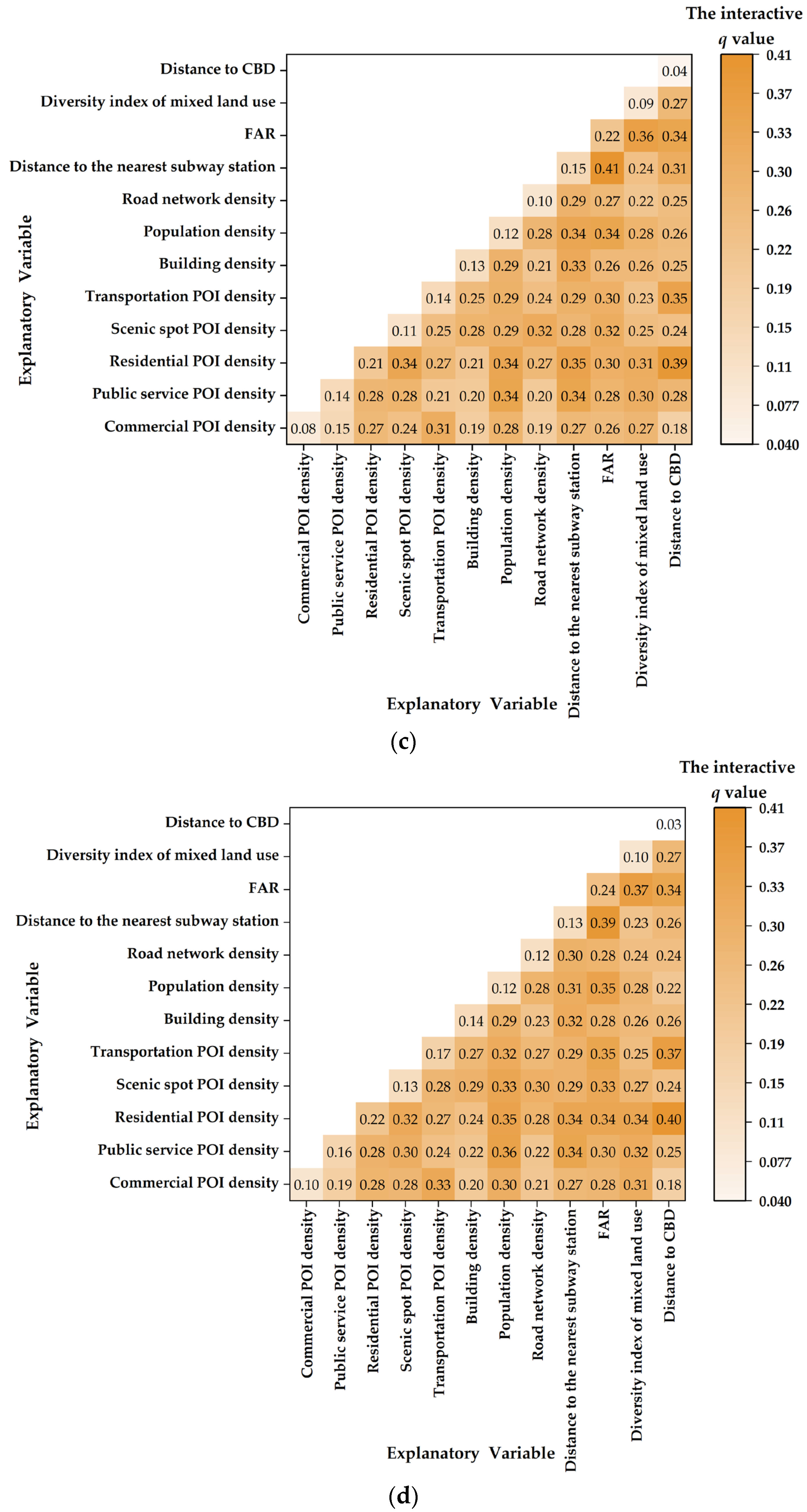
4.4. Interactive Detection Results

The interaction detector explores an interaction by comparing the q values of the interaction and the two single variables. In the study on the influencing factors of the ridership of rider-hailing in Chengdu, the interaction between two factors showed two kinds of relationship, namely nonlinear enhancement and double-factor enhancement. This indicates that the contribution of the interaction between two factors on the ridership of ride-hailing was enhanced to varying degrees compared with the single-factor effect, and the results are shown in Figure 10.

In the morning peak hours, the three interactions with the highest q values that affected the pick-up ridership were the diversity index of mixed land use ∩ commercial POI density, the diversity index of mixed land use ∩ residential POI density, and the transportation POI density ∩ building density, and the corresponding interactive q values were 0.40, 0.38, and 0.37, respectively. The interactions between two influencing factors (population density and diversity index of mixed land use degree) had relatively high interactive impacts on the pick-up ridership of ride-hailing. The three interactions with the highest q values that affected the drop-off ridership were the distance to the CBD ∩ residential POI density, the distance to the CBD ∩ distance to the nearest subway station, and the FAR ∩ distance to the nearest subway station, and the corresponding interactive q values were 0.41, 0.40, and 0.40, respectively. The interactions between two influencing factors (distance to the nearest subway station and residential POI density) had relatively high interactive impacts on the drop-off ridership of ride-hailing. The traffic management department should pay more attention to the road traffic around the subway station and the areas with a high residential POI density in the morning peak hours to avoid traffic congestion caused by the concentration of drop-off demands.

In the evening peak hours, the three interactions with the highest q values that affected the pick-up ridership were the FAR ∩ distance to the nearest subway station, the distance to the CBD ∩ residential POI density, and the diversity index of mixed land use ∩ FAR, and the corresponding interactive q values were 0.41, 0.39, and 0.36, respectively. The interactions among three influencing factors (distance to the nearest subway station, population density, and residential POI density) had relatively high interactive impacts on the pick-up ridership of ride-hailing. The three interactions with the highest q values that affected the drop-off ridership were the distance to the CBD ∩ residential POI density, the distance to the nearest subway station ∩ FAR, and the transportation POI density ∩ distance to the CBD, and the corresponding interactive q values were 0.40, 0.39, and 0.37, respectively. The interactions among three influencing factors (population density, distance to the CBD, and residential POI density) had relatively high interactive impacts on the drop-off ridership of ride-hailing. Urban planners should pay attention to adjusting the layout and scale of residential land and office land, strive to achieve a balance between work and residence, and improve urban traffic efficiency.

The factor detector results showed that the FAR had the highest contribution to the ride-hailing ridership. The interaction results between the FAR and the other three main influencing factors are shown in

Table 6. The interactive detector results of dominant variables.

Time	Dependent Variable	Dominant Factor (q Value)	Interaction Factors	Interactive q Value	Percent Change in q Value after Interaction
Morning peak hours	Pick-ups of ride-hailing vehicles	FAR (0.23)	Diversity index of mixed land use ∩ FAR;	0.39	+69.6%
			Distance to the nearest subway station ∩ FAR;	0.37	+60.9%
			Transportation POI density ∩ FAR	0.35	+52.2%
	Drop-offs of ride-hailing vehicles	FAR (0.17)	Distance to the nearest subway station ∩ FAR;	0.40	+135.3%
			Diversity index of mixed land use ∩ FAR;	0.32	+88.2%
			Distance to CBD ∩ FAR	0.31	+82.4%
Evening peak hours	Pick-ups of ride-hailing vehicles	FAR (0.22)	Distance to the nearest subway station ∩ FAR;	0.41	+86.4%
			Diversity index of mixed land use ∩ FAR;	0.36	+63.6%
			Distance to CBD ∩ FAR	0.34	+54.5%
	Drop-offs of ride-hailing vehicles	FAR (0.24)	Distance to the nearest subway station ∩ FAR;	0.39	+62.5%
			Diversity index of mixed land use ∩ FAR;	0.37	+54.2%
			Population density ∩ FAR	0.35	+45.8%

. For the pick-up ridership in the morning peak hours, the three interactions with the highest interactive q value were: the diversity index of mixed land use ∩ FAR, the distance to the subway station ∩ FAR, and the transportation POI density ∩ FAR, with contributions of 39%, 37%, and 35%, respectively, and the percent changes in the q values after the interaction were +69.6%, +60.9%, and +52.2%, respectively. Computed with the factor detector, the q values of the distance to the nearest subway station and the diversity index of mixed land use were less than the q value of the transportation POI density, but the influence was greatly enhanced after the interaction with the FAR. The q value represents the contribution of the explanatory variable to the spatial distribution of the ridership of ride-hailing [40], which indicates that the spatial distribution of the pick-ups in the morning peak hours was more than 35% consistent with the spatial distribution of the interaction between the FAR and the three influencing factors just mentioned. This shows that during the morning peak hours, the vehicle dispatching needs to be adjusted to allocate more vehicles to the three types of areas: (1) areas with a high FAR and high diversity index of mixed land use, (2) areas with a high FAR and short distance to the subway station, and (3) areas with a high FAR and high transportation POI density. In addition, the “diversity index of mixed land use ∩ FAR” had the strongest interaction for ride-hailing pick-ups in the morning peak hours. The operators of ride-hailing should pay special attention to the vehicle allocation and the temporary roadside parking in such areas to reduce the impact on non-motor vehicles. Attention should also be paid to vehicle allocation in areas with a high FAR around public transport stations, and planning and design for these areas should be considered to reduce the spatial conflict between public transport and ride-hailing.

For the drop-off ridership in the morning peak hours, the three interactions with the highest interactive q values were: the distance to the nearest subway station ∩ FAR, the diversity index of mixed land use ∩ FAR, and the distance to the CBD ∩ FAR, with contributions of 40%, 32%, and 31%, respectively, and the percent changes in the q values after the interaction were +135.3%, +88.2%, and +82.4%, respectively. This shows that during the morning peak hours, attention should be paid to the following areas: areas with a high FAR and short distance to the subway station, areas with a high FAR and high diversity index of mixed land use, and areas with a high FAR and short distance to the CBD. Traffic management should be set to prevent traffic congestion caused by the high-density demand of ride-hailing. It is worth noting that the “distance to the nearest subway station ∩ FAR” had the strongest interaction for the drop-off ridership in the morning peak hours. The traffic management department should pay attention to the traffic management of high FAR areas near the subway station in the morning peak hours.

For the pick-up ridership in the evening peak hours, the three interactions with the highest interactive q values were: the distance to the nearest subway station ∩ FAR, the diversity index of mixed land use ∩ FAR, and the distance to the CBD ∩ FAR, with contributions of 41%, 36%, and 34%, respectively, and the percent changes in the q values after the interaction were +86.4%, +63.6%, and +54.5%, respectively. This shows that during the evening peak hours, the ride-hailing operator needs to adjust the vehicle scheduling and vehicles should be allocated to the following areas: (1) areas with a high diversity index of mixed land use and a high FAR, (2) areas near the subway stations and with a high FAR, and (3) areas near the CBD and with a high FAR. It is worth noting that the q value of the distance from the CBD computed with the factor detector was 0.04, but the interaction between the distance from the CBD and the residential POI density had a high q value of 0.39 with an increase of 875%, which indicates that the ride-hailing company should allocate more vehicles to residential communities near the CBD during the evening peak hours. In addition, the q value of the single-factor effect of transportation POI density was 0.14, and the interaction between the transportation POI density and the distance to the CBD had a high q value of 0.35 with an increase of 150%. This indicates that an increase in the transportation POI density near the CBD will result in more ride-hailing demand.

For the drop-off ridership in the evening peak hours, the three interactions with the highest interactive q values were: the distance to the nearest subway station ∩ FAR, the diversity index of mixed land use ∩ FAR, and the population density ∩ FAR, with contributions of 39%, 37%, and 35%, respectively, and the percent changes in the q values after the interaction were +62.5%, +54.2%, and +45.8%, respectively. It is worth noting that the q value of the single-factor effect of the distance to the CBD was 0.03, and the q value of the interaction with the residential POI density was 0.40, which is 1.233% higher than the single-factor effect. This indicates that an increase in the residential POI density near the CBD will result in more ride-hailing demand.

5. Conclusions and Future Work

Based on the order data of ride-hailing in Chengdu, this study used the NSR method and OPGD model to calculate the optimal grid scale and combined the “5D” built-environment influencing factors to build an impact factor model of ride-hailing in the morning and evening peak hours. By comparing the q value results of the geographical detector, the optimal data discretization method was found and the single-factor and interactive effects of the built environment on ride-hailing were analyzed. The main findings and conclusions are as follows: (1) The results of research on the impact of the built environment on the ridership of ride-hailing vary with different research scales. The average value of the calculated results of the NSR and OPGD model shows that the suggested grid scale for studying the impact of the built environment on the pick-up and drop-off ridership during the morning and evening peak hours in Chengdu is 1100 m. The proposed grid scale can provide a basis for the partitioning management and scheduling optimization of ride-hailing. (2) The factor detector results show that the FAR, the residential POI density, and the transportation POI density are the major contributors to ride-hailing ridership in the morning and evening peak hours. The interactive detection results show that the interactions of the diversity index of mixed land use ∩ FAR, the distance to the nearest subway station ∩ FAR, the transportation POI density ∩ FAR, and the distance to the CBD ∩ FAR made a higher contribution to the ride-hailing ridership than the single-factor effect of the FAR computed by the factor detector. The “distance to the nearest subway station ∩ FAR” had the strongest interaction contribution, with a 135.3% increase in the q value compared to the single-factor effect of the FAR computed by the factor detector for the drop-off ridership in the morning peak hours. For the pick-up ridership in the evening peak hours, the interaction between the distance from the CBD and the residential POI density increased the contribution by 875% compared to the single-factor effect of the distance from the CBD, and the interaction between the transportation POI density and the distance to the CBD increased the contribution by 150% compared to the single-factor effect of the transportation POI density. For the drop-off ridership in the evening peak hours, the interaction between the distance to the CBD and the residential POI density increased the contribution by 1.233% compared to the single-factor effect of the distance to the CBD. Based on the results of the interactive detection, the effect of the interactions among built-environment explanatory variables on the demand for ride-hailing should not be ignored. In the process of adjusting the regional global ride-hailing demand, the ranking results of the importance and interaction of the built-environment explanatory variables have important reference significance for formulating the priority renewal order of the built-environment factors. The interaction results for the explanatory variables of the built environment with relatively high contribution degrees provide a basis for proposing a scientific combination scheme of built-environment factors when adjusting the size of the demand for ride-hailing in a specific area.

Although this study makes up for some gaps in the research investigating the built-environment impact on the ridership of ride-hailing, it still has the following limitations: (1) We took POI point data as the basic data, ignoring the impact of the actual built-up area of each influencing factor on the model results. In future research, the POI point density could be corrected through the area of interest (AOI) of the built environment to make the research results more real and accurate. (2) The amount of data obtained in this paper was limited. In the future, more in-depth travel behavior research can be carried out by adding individual and family characteristic explanatory variables in combination with the residents’ travel survey in the form of small samples. (3) For the zoning effect of the MAUP problem, this study only considered the spatial grid division method, and did not consider the impact of the traffic analysis zone or other block division methods. (4) We suggest that urban planners put up with some planning strategies to increase the variance in the FAR and the residential POI density within the whole study area and reduce the variance in the sub-region, but specific strategies require further study. (5) The data of online booking orders we obtained in 2016 might not represent the actual situation in 2022. In addition to the impact of COVID-19, the Chinese government adopted relevant policies to reduce residents’ travel from 2020 to 2022, which must have had a great impact on the number of ride-hailing orders. We hope to obtain the latest ride-hailing data from Chengdu to verify the results of this research.

References

1. He, Z.B. Portraying ride-hailing mobility using multi-day trip order data: A case study of Beijing, China. Transp. Res. Part A Policy Pract. 2021, 146, 152–169. [Google Scholar] [CrossRef]
2. Li, Z.R.; Hong, Y.L.; Zhang, Z.J. An empirical analysis of on-demand ride-sharing and traffic congestion. In Proceedings of the 50th Annual Hawaii International Conference on System Sciences (HICSS), Waikoloa Village, HI, USA, 3–7 January 2017; pp. 4–13. [Google Scholar]
3. Gao, J.; Ma, S.F.; Li, L.L.; Zuo, J.; Du, H.B. Does travel closer to TOD have lower CO2 emissions? Evidence from ride-hailing in Chengdu, China. J. Environ. Manag. 2022, 308, 114636. [Google Scholar] [CrossRef] [PubMed]
4. Tirachini, A. Ride-hailing, travel behaviour and sustainable mobility: An international review. Transportation 2020, 47, 2011–2047. [Google Scholar] [CrossRef]
5. Cervero, R.; Kockelman, K. Travel demand and the 3Ds: Density, diversity, and design. Transp. Res. Part D Transp. Environ. 1997, 2, 199–219. [Google Scholar] [CrossRef]
6. Lavieri, P.S.; Bhat, C.R. Investigating objective and subjective factors influencing the adoption, frequency, and characteristics of ride-hailing trips. Transp. Res. Part C Emerg. Technol. 2019, 105, 100–125. [Google Scholar] [CrossRef]
7. Zhai, G.; Yang, H.; Pan, R.; Wang, J.; Xiong, Y. Usage characteristics and mode choice transitions of ride-hailing users in Chengdu, China. In Proceedings of the 5th International Conference on Transportation Information and Safety, ICTIS 2019, Liverpool, UK, 14–17 July 2019; pp. 1233–1238. [Google Scholar]
8. Loa, P.; Habib, K.N. Examining the influence of attitudinal factors on the use of ride-hailing services in Toronto. Transp. Res. Part A Policy Pract. 2021, 146, 13–28. [Google Scholar] [CrossRef]
9. Acheampong, R.A.; Siiba, A.; Okyere, D.K.; Tuffour, J.P. Mobility-on-demand: An empirical study of internet-based ride-hailing adoption factors, travel characteristics and mode substitution effects. Transp. Res. Part C Emerg. Technol. 2020, 115, 102638. [Google Scholar] [CrossRef]
10. Zhang, B.; Chen, S.; Ma, Y.; Li, T.; Tang, K. Analysis on spatiotemporal urban mobility based on online car-hailing data. J. Transp. Geogr. 2020, 82, 102568. [Google Scholar] [CrossRef]
11. Handy, S.L.; Boarnet, M.G.; Ewing, R.; Killingsworth, R.E. How the built environment affects physical activity—Views from urban planning. Am. J. Prev. Med. 2002, 23, 64–73. [Google Scholar] [CrossRef] [PubMed]
12. Kahn, M.E. A Review of Travel by Design: The Influence of Urban Form on Travel. Reg. Sci. Urban Econ. 2002, 32, 275–277. [Google Scholar] [CrossRef]
13. Gao, F.; Li, S.Y.; Tan, Z.Z.; Wu, Z.F.; Zhang, X.M.; Huang, G.P.; Huang, Z.W. Understanding the modifiable areal unit problem in dockless bike sharing usage and exploring the interactive effects of built environment factors. Int. J. Geogr. Inf. Sci. 2021, 35, 1905–1925. [Google Scholar] [CrossRef]
14. Bi, H.; Ye, Z.R.; Wang, C.; Chen, E.H.; Li, Y.W.; Shao, X.M. How Built Environment Impacts Online Car-Hailing Ridership. Transp. Res. Rec. 2020, 2674, 745–760. [Google Scholar] [CrossRef]
15. Wang, S.C.; Noland, R.B. Variation in ride-hailing trips in Chengdu, China. Transp. Res. Part D Transp. Environ. 2021, 90, 102596. [Google Scholar] [CrossRef]
16. Openshaw, S. The modifiable areal unit problem. Concepts Tech. Mod. Geogr. 1984, 38, 1–41. [Google Scholar]
17. Lee, S.I.; Lee, M.; Chun, Y.; Griffith, D.A. Uncertainty in the effects of the modifiable areal unit problem under different levels of spatial autocorrelation: A simulation study. Int. J. Geogr. Inf. Sci. 2019, 33, 1135–1154. [Google Scholar] [CrossRef]
18. Chen, L.; Gao, Y.; Zhu, D.; Yuan, Y.H.; Liu, Y. Quantifying the scale effect in geospatial big data using semi-variograms. PLoS ONE 2019, 14, e0225139. [Google Scholar] [CrossRef] [PubMed]
19. Openshaw, S. A geographical solution to scale and aggregation problems in region-building, partitioning and spatial modelling. Trans. Inst. Br. Geogr. 1977, 2, 459–472. [Google Scholar] [CrossRef]
20. Guo, L.; Gong, H.L.; Zhu, F.; Zhu, L.; Zhang, Z.X.; Zhou, C.F.; Gao, M.L.; Sun, Y.K. Analysis of the Spatiotemporal Variation in Land Subsidence on the Beijing Plain, China. Remote Sens. 2019, 11, 1170. [Google Scholar] [CrossRef]
21. Altan, M.F.; Ayozen, Y.E. The Effect of the Size of Traffic Analysis Zones on the Quality of Transport Demand Forecasts and Travel Assignments. Period. Polytech. Civ. Eng. 2018, 62, 971–979. [Google Scholar] [CrossRef]
22. Dong, H.H.; Wu, M.C.; Ding, X.Q.; Chu, L.Y.; Jia, L.M.; Qin, Y.; Zhou, X.S. Traffic zone division based on big data from mobile phone base stations. Transp. Res. Part C Emerg. Technol. 2015, 58, 278–291. [Google Scholar] [CrossRef]
23. Sun, G.D.; Chang, B.F.; Zhu, L.; Wu, H.; Zheng, K.; Liang, R.H. TZVis: Visual analysis of bicycle data for traffic zone division. J. Vis. 2019, 22, 1193–1208. [Google Scholar] [CrossRef]
24. Tao, R.; Liu, J.; Song, Y.Q.; Peng, R.; Zhang, D.L.; Qiao, J.G. Detection and Optimization of Traffic Networks Based on Voronoi Diagram. Discret. Dyn. Nat. Soc. 2021, 2021, 5550315. [Google Scholar] [CrossRef]
25. Wang, Z.; Song, J.; Zhang, Y.; Li, S.; Jia, J.; Song, C. Spatial Heterogeneity Analysis for Influencing Factors of Outbound Ridership of Subway Stations Considering the Optimal Scale Range of “7D” Built Environments. Sustainability 2022, 14, 16314. [Google Scholar] [CrossRef]
26. Liu, X.; Kang, C.G.; Gong, L.; Liu, Y. Incorporating spatial interaction patterns in classifying and understanding urban land use. Int. J. Geogr. Inf. Sci. 2016, 30, 334–350. [Google Scholar] [CrossRef]
27. Pei, T.; Sobolevsky, S.; Ratti, C.; Shaw, S.L.; Li, T.; Zhou, C.H. A new insight into land use classification based on aggregated mobile phone data. Int. J. Geogr. Inf. Sci. 2014, 28, 1988–2007. [Google Scholar] [CrossRef]
28. Song, Y.Z.; Wang, J.F.; Ge, Y.; Xu, C.D. An optimal parameters-based geographical detector model enhances geographic characteristics of explanatory variables for spatial heterogeneity analysis: Cases with different types of spatial data. GIsci. Remote Sens. 2020, 57, 593–610. [Google Scholar] [CrossRef]
29. Munoz, J.D.; Kravchenko, A. Deriving the optimal scale for relating topographic attributes and cover crop plant biomass. Geomorphology 2012, 179, 197–207. [Google Scholar] [CrossRef]
30. Du, M.Y.; Li, X.F.; Kwan, M.P.; Yang, J.Z.; Liu, Q.Y. Understanding the Spatiotemporal Variation of High-Efficiency Ride-Hailing Orders: A Case Study of Haikou, China. ISPRS Int. J. Geo Inf. 2022, 11, 42. [Google Scholar] [CrossRef]
31. Zhuo, Y.; Mark, L.F.; Shanjiang, Z.; Jina, M.; Arefeh, N.; Lei, Z. Analysis of Washington, DC taxi demand using GPS and land-use data. J. Transp. Geogr. 2018, 66, 35–44. [Google Scholar]
32. Li, T.; Jing, P.; Li, L.C.; Sun, D.Z.; Yan, W.B. Revealing the Varying Impact of Urban Built Environment on Online Car-Hailing Travel in Spatio-Temporal Dimension: An Exploratory Analysis in Chengdu, China. Sustainability 2019, 11, 1336. [Google Scholar] [CrossRef]
33. Zhang, X.X.; Huang, B.; Zhu, S.Z. Spatiotemporal Varying Effects of Built Environment on Taxi and Ride-Hailing Ridership in New York City. ISPRS Int. J. Geo Inf. 2020, 9, 475. [Google Scholar] [CrossRef]
34. Wang, S.; Wang, J.J.; Li, W.J.; Fan, J.L.; Liu, M.Y. Revealing the Influence Mechanism of Urban Built Environment on Online Car-Hailing Travel considering Orientation Entropy of Street Network. Discret. Dyn. Nat. Soc. 2022, 2022, 3888800. [Google Scholar] [CrossRef]
35. Nair, G.S.; Bhat, C.R.; Batur, I.; Pendyala, R.M.; Lam, W.H.K. A model of deadheading trips and pick-up locations for ride-hailing service vehicles. Transp. Res. Part A Policy Pract. 2020, 135, 289–308. [Google Scholar] [CrossRef]
36. Zhao, G.W.; Li, Z.T.; Shang, Y.Z.; Yang, M.Z. How Does the Urban Built Environment Affect Online Car-Hailing Ridership Intensity among Different Scales? Int. J. Environ. Res. Public Health 2022, 19, 5325. [Google Scholar] [CrossRef]
37. Sabouri, S.; Park, K.; Smith, A.; Tian, G.; Ewing, R. Exploring the influence of built environment on Uber demand. Transp. Res. Part D Transp. Environ. 2020, 81, 102296. [Google Scholar] [CrossRef]
38. Tu, M.; Li, W.; Orfila, O.; Li, Y.; Gruyer, D. Exploring nonlinear effects of the built environment on ridesplitting: Evidence from Chengdu. Transp. Res. Part D Transp. Environ. 2021, 93, 102776. [Google Scholar] [CrossRef]
39. Müller, J.; Correia, G.H.D.; Bogenberger, K. An Explanatory Model Approach for the Spatial Distribution of Free-Floating Carsharing Bookings: A Case-Study of German Cities. Sustainability 2017, 9, 1290. [Google Scholar] [CrossRef]
40. Wang, J.F.; Li, X.H.; Christakos, G.; Liao, Y.L.; Zhang, T.; Gu, X.; Zheng, X.Y. Geographical Detectors-Based Health Risk Assessment and its Application in the Neural Tube Defects Study of the Heshun Region, China. Int. J. Geogr. Inf. Sci. 2010, 24, 107–127. [Google Scholar] [CrossRef]
41. Wang, J.F.; Hu, Y. Environmental health risk detection with GeogDetector. Environ. Model. Softw. 2012, 33, 114–115. [Google Scholar] [CrossRef]
42. He, J.H.; Pan, Z.Z.; Liu, D.F.; Guo, X.N. Exploring the regional differences of ecosystem health and its driving factors in China. Sci. Total Environ. 2019, 673, 553–564. [Google Scholar] [CrossRef]
43. Liao, Y.L.; Wang, J.F.; Wu, J.L.; Driskell, L.; Wang, W.Y.; Zhang, T.; Gu, X.; Zheng, X.Y. Spatial analysis of neural tube defects in a rural coal mining area. Int. J. Environ. Health Res. 2011, 20, 439–450. [Google Scholar] [CrossRef] [PubMed]
44. Ding, Y.T.; Zhang, M.; Qian, X.Y.; Li, C.R.; Chen, S.; Wang, W.W. Using the geographical detector technique to explore the impact of socioeconomic factors on PM2.5 concentrations in China. J. Clean. Prod. 2019, 211, 1480–1490. [Google Scholar] [CrossRef]
45. Yue, H.; Hu, T. Geographical Detector-Based Spatial Modeling of the COVID-19 Mortality Rate in the Continental United States. Int. J. Environ. Res. Public Health 2021, 18, 6832. [Google Scholar] [CrossRef]
46. Huang, J.X.; Wang, J.F.; Bo, Y.C.; Xu, C.D.; Hu, M.G.; Huang, D.C. Identification of Health Risks of Hand, Foot and Mouth Disease in China Using the Geographical Detector Technique. Int. J. Environ. Res. Public Health 2014, 11, 3407–3423. [Google Scholar] [CrossRef] [PubMed]
47. Wang, Z.L.; Liu, L.; Zhou, H.L.; Lan, M.X. Crime Geographical Displacement: Testing Its Potential Contribution to Crime Prediction. ISPRS Int. J. Geo Inf. 2019, 8, 383. [Google Scholar] [CrossRef]
48. Wan, T.; Shi, B.H. Exploring the Interactive Associations between Urban Built Environment Features and the Distribution of Offender Residences with a GeoDetector Model. ISPRS Int. J. Geo Inf. 2022, 11, 369. [Google Scholar] [CrossRef]
49. Qiao, P.W.; Lei, M.; Guo, G.H.; Yang, J.; Zhou, X.Y.; Chen, T.B. Quantitative Analysis of the Factors Influencing Soil Heavy Metal Lateral Migration in Rainfalls Based on Geographical Detector Software: A Case Study in Huanjiang County, China. Sustainability 2017, 9, 1227. [Google Scholar] [CrossRef]
50. Qiao, P.W.; Yang, S.C.; Lei, M.; Chen, T.B.; Dong, N. Quantitative analysis of the factors influencing spatial distribution of soil heavy metals based on geographical detector. Sci. Total Environ. 2019, 664, 392–413. [Google Scholar] [CrossRef]
51. Wu, R.N.; Zhang, J.Q.; Bao, Y.H.; Zhang, F. Geographical Detector Model for Influencing Factors of Industrial Sector Carbon Dioxide Emissions in Inner Mongolia, China. Sustainability 2016, 8, 149. [Google Scholar] [CrossRef]
52. Zhang, X.L.; Zhao, Y. Identification of the driving factors’ influences on regional energy-related carbon emissions in China based on geographical detector method. Environ. Sci. Pollut. Res. 2018, 25, 9626–9635. [Google Scholar] [CrossRef]
53. Shannon, C.E.; Weaver, W. A Mathematical Theory of Communication. Philos. Rev. 1949, 5, 3–55. [Google Scholar]
54. Curran, P.J.; Atkinson, P.M. Geostatistics and remote sensing. Prog. Phys. Geogr. 1998, 22, 61–78. [Google Scholar] [CrossRef]
55. Li, H.D.; Shen, W.S.; Zou, C.X.; Jiang, J.; Fu, L.N.; She, G.H. Spatio-temporal variability of soil moisture and its effect on vegetation in a desertified aeolian riparian ecotone on the Tibetan Plateau, China. J. Hydrol. 2013, 479, 215–225. [Google Scholar] [CrossRef]
56. Ly, S.; Charles, C.; Degre, A. Geostatistical interpolation of daily rainfall at catchment scale: The use of several variogram models in the Ourthe and Ambleve catchments, Belgium. Hydrol. Earth Syst. Sci. 2011, 15, 2259–2274. [Google Scholar] [CrossRef]
57. Zhang, P.P.; Wang, Y.Q.; Sun, H.; Qi, L.J.; Liu, H.; Wang, Z. Spatial variation and distribution of soil organic carbon in an urban ecosystem from high-density sampling. Catena 2021, 204, 105364. [Google Scholar] [CrossRef]
58. Yan, T.T.; Zhao, W.J.; Zhu, Q.K.; Xu, F.J.; Gao, Z.K. Spatial distribution characteristics of the soil thickness on different land use types in the Yimeng Mountain Area, China. Alex. Eng. J. 2021, 60, 511–520. [Google Scholar] [CrossRef]
59. Ghorbani, M.A.; Deo, R.C.; Kashani, M.H.; Shahabi, M.; Ghorbani, S. Artificial intelligence-based fast and efficient hybrid approach for spatial modelling of soil electrical conductivity. Soil Tillage Res. 2019, 186, 152–164. [Google Scholar] [CrossRef]
60. Barkat, A.; Bouaicha, F.; Bouteraa, O.; Mester, T.; Ata, B.; Balla, D.; Rahal, Z.; Szabo, G. Assessment of Complex Terminal Groundwater Aquifer for Different Use of Oued Souf Valley (Algeria) Using Multivariate Statistical Methods, Geostatistical Modeling, and Water Quality Index. Water 2021, 13, 1609. [Google Scholar] [CrossRef]
61. Trangmar, B.B.; Yost, R.S.; Uehara, G. Application of Geostatistics to Spatial Studies of Soil Properties. Adv. Agron. 1986, 38, 45–94. [Google Scholar]
62. Van Groenigen, J.W. The influence of variogram parameters on optimal sampling schemes for mapping by kriging. Geoderma 2000, 97, 223–236. [Google Scholar] [CrossRef]
63. Liu, D.W.; Wang, Z.M.; Zhang, B.; Song, K.S.; Li, X.Y.; Li, J.P.; Li, F.; Duan, H.T. Spatial distribution of soil organic carbon and analysis of related factors in croplands of the black soil region, Northeast China. Agric. Ecosyst. Environ. 2006, 113, 73–81. [Google Scholar] [CrossRef]
64. Ahmadi, S.H.; Sedghamiz, A. Geostatistical analysis of spatial and temporal variations of groundwater level. Environ. Monit. Assess. 2007, 129, 277–294. [Google Scholar] [CrossRef]
65. Wang, J.F.; Xu, C.D. Geodetector: Principle and prospect. Acta Geogr. Sin. 2017, 72, 116–143. [Google Scholar]
66. Kodinariya, T.M.; Makwana, P.R. Review on determining number of Cluster in K-Means Clustering. Int. J. Adv. Res. Comput. Sci. Manag. Stud. 2013, 1, 90–95. [Google Scholar]
67. Koenker, R.; Bassett, G.W. Regression quantiles. Econometrica 1978, 46, 211–244. [Google Scholar] [CrossRef]
68. Hall, J.D.; Palsson, C.; Price, J. Is Uber a substitute or complement for public transit? J. Urban Econ. 2018, 108, 36–50. [Google Scholar] [CrossRef] [Green Version]
Figure 1. The study area.
Applsci 13 02180 g001
Figure 2. The schematic diagram of space unit division.
Applsci 13 02180 g002
Figure 3. A diagram of the semi-variogram.
Applsci 13 02180 g003
Figure 4. Hourly variation in ridership of ride-hailing on weekdays.
Applsci 13 02180 g004
Figure 5. The distribution of ride-hailing pick-ups and drop-offs in Chengdu. (a) Pick-ups in the morning peak hours; (b) drop-offs in the morning peak hours; (c) pick-ups in the evening peak hours; and (d) drop-offs in the evening peak hours.
Applsci 13 02180 g005
Figure 6. Comparison of size effects and NSR of explanatory variables. (a) Pick-up ridership in the morning peak hours; (b) drop-off ridership in the morning peak hours; (c) pick-up ridership in the evening peak hours; and (d) drop-off ridership in the evening peak hours.
Applsci 13 02180 g006
Figure 7. Comparison of 90% quantile of q values for explanatory variables under different grid sizes.
Applsci 13 02180 g007
Figure 8. Contribution of single explanatory variables on pick-up and drop-off ridership in the morning peak hours by the factor detector.
Applsci 13 02180 g008
Figure 9. Contribution of single explanatory variables on pick-up and drop-off ridership in the evening peak hours by the factor detector.
Applsci 13 02180 g009
Figure 10. The results of the interactive detector for built-environment variables. (a) Pick-ups in the morning peak hours; (b) drop-offs in the morning peak hours; (c) pick-ups in the evening peak hours; and (d) drop-offs in the evening peak hours.
Applsci 13 02180 g010aApplsci 13 02180 g010b