Article

Routing, Modulation Format, Spatial Lane, and Spectrum Block Assignment in Static Spatial Channel Networks

School of Electronic and Information Engineering, Beijing Jiaotong University, Beijing 100044, China
*
Author to whom correspondence should be addressed.
Appl. Sci. 2023, 13(4), 2105; https://doi.org/10.3390/app13042105
Submission received: 29 November 2022 / Revised: 3 February 2023 / Accepted: 3 February 2023 / Published: 6 February 2023

Abstract

:
Spatial channel networks (SCNs) and related key technologies have been proposed to increase the capacity and flexibility of optical networks. We define the network resource allocation problem in a static SCN as the routing, modulation format (MF), spatial lane, and spectrum block assignment (RMSSA) problem and try to solve it. In this paper, we derive the relationship between the traffic bit rate, the transmission distance of optical channels, and MFs in SCNs, and obtain the adoption method of MFs. In addition, we introduce conversion nodes (CNs) into SCNs to perform a modulation format conversion (MFC) for more efficient use of network resources. Moreover, the RMSSA problem in static SCNs is modeled, and heuristic spatial lane and spectrum block minimization based on simulated annealing (LBMSA) algorithm is proposed to solve the RMSSA problem. Simulation results show that when the throughput of SCNs is small, the LBMSA algorithm can carry traffic requests with the least amount of network resources and maximize the network resource utilization. When the network throughput is high, the LBMSA algorithm is more inclined to carry all requests rather than efficient transmission. We also show that network resource utilization can be improved with the LBMSA algorithm by setting CNs to perform the MFC.

1. Introduction

Nowadays, society is in a rapidly developing information age, and the development of new broadband-intensive industries, such as the internet of things, cloud services, and data centers not only prompt network traffic requests to grow at a high rate but also place higher requirements on the flexible and dynamic transmission capability of optical networks. Moreover, assuming that router blade capacities grow steadily at 40% per year, then a single transceiver could carry ~100 terabit per second (Tb/s) of such extra-bitrate traffic requests by 2030, and the entire fiber would be equivalent to a logical point-to-point interface at that time [1]. Elastic optical networks (EONs) divide the fixed wavelengths in traditional wavelength division multiplexing (WDM) optical networks into frequency slots (FSs) of finer granularity [2,3,4,5], which can effectively improve network flexibility and spectrum resource utilization, thus increasing the throughput of the network. Nevertheless, EONs are still based on single-core fibers (SMFs), and the transmission capacity of existing SMFs is close to the Shannon capacity. It is difficult for EONs to cope with such extra-bitrate traffic requests.
Multi-core fibers (MCFs) use the technology of embedding multiple single-mode fiber cores into the fiber cladding, an MCF is equivalent to a corresponding number of SMFs, so it can carry more service requirements without much increase in network costs, and it is easy to achieve exponential growth in the network capacity. Researchers have introduced space division multiplexing-based technology into EONs, which have the advantages of a high throughput, high flexibility, low crosstalk, and core independence. Although SDM-EONs can significantly increase the network capacity, the use of SDM fibers means ultra-scale deployment of very large-size scalable reconfigurable optical add-drop multiplexers (ROADMs), which implies higher costs and more complex network node structures. Furthermore, new optical node technologies are still limited to solving problems from a single WDM layer perspective, using fine-granular key technologies, such as wavelength switching. Taking these considerations into account, spatial channel networks (SCNs) have been creatively proposed to address these aforementioned problems [6,7]. In [6,7], the idea of introducing optical bypass into optical networks to build hierarchical IP-over-WDM network architectures based on ROADMs/WXCs, is borrowed by SCNs. Hierarchical IP-over-WDM-over-SDM network architectures are built by introducing spatial bypass based on spatial channel cross-connects (SXCs) into the SDM layer. SCNs replace wavelength switching with spatial switching of coarser granularity, evolve the optical layer explicitly into a WDM layer and an SDM layer, and transform optical nodes into hierarchical optical cross-connects (HOXCs) consisting of SXCs and WXCs. The spatial switching of coarser granularity indicates that SCNs have a large network capacity. The use of HOXCs can reduce the cost and simplify the network node structure. M. Jinno et al. have conducted serious studies on SCN architectures and the enabling technologies [8,9,10,11,12,13,14,15,16] as well as evaluated scalability, reliability, and techno economics [10,11,12,13] to ensure SCNs be promising for reliable and cost-effective optical architectures toward the forthcoming SDM era.
Since SCNs are highly promising optical network architectures, it is necessary to further study the network resource allocation problem in SCNs. With the evolution of optical networks from WDM networks to EONs, SDM-EONs, and then to SCNs, network resource units that need to be allocated have also changed accordingly. The routing and wavelength assignment (RWA) problem is the key issue of resource allocation in WDM networks. Network resource units to be allocated in EONs are changed from wavelengths of WDM to FSs, and the key problem is converted from the RWA problem to the routing and spectrum assignment (RSA) problem [17]. The resource allocation problem in SDM-EONs treating a fiber core as a new resource allocation variable is called the routing, core, and spectrum assignment (RCSA) problem. The traffic request suffers less transmission impairment when transmitted over short distance links, and can meet the transmission quality requirements of different modulation formats (MFs) at the receiving end. Therefore, using the same MF on links of different lengths inevitably leads to a waste of network spectrum resources and reduces the spectrum resource utilization. Therefore, flexible MFs can be considered when solving the network resource allocation problem. The RSA problem of EONs and the RCSA problem of SDM-EONs, considering selecting an appropriate MF for a signal to improve network resource utilization, are expanded into the routing, modulation format, and spectrum assignment (RMSA) problem and the routing, core, spectrum, and modulation format assignment (RCSMA) problem. According to these research methods, when solving the network resource allocation problem in SCNs, suitable network resource units need to be selected and flexible MFs can be considered to be utilized.

2. Related Works

As shown in Table 1, we sort out the network resource allocation methods applied to different optical network architectures, which provides us with ideas for studying the resource allocation problem in SCNs.
RSA in EONs. The EON architecture is considered one of the most promising directions for optical networks [5]. The RSA problem of EONs refers to finding a suitable routing path for a traffic request between its source and destination nodes while satisfying both the spectrum continuity constraint and the spectrum contiguity constraint and allocating the appropriate spectrum resources to establish an optical connection based on the principle of maximizing the spectrum resource utilization [18]. Integer linear programming (ILP) models and variant forms [19,20] have been used to solve the static RSA problem, and intelligent optimization algorithms, such as the tabu search [21], particle swarm optimization [22], differential evolution [23], simulated annealing (SA) [24], and bee colony optimization [25] have been widely adopted. Dynamically establishing and removing optical connections adds a great deal of difficulty to solving the dynamic RSA problem. Heuristic algorithms are frequently used to solve dynamic RSA problems [26,27]. Meanwhile, intelligent algorithms, such as backpropagation neural networks [28], deep reinforcement learning [29], and asynchronous advantage actor-critic algorithms [30] have also been applied to solve the problem, but relatively little research has been carried out in this area.
RCSA in SDM-EONs. To further increase the signal transmission rate and capacity of the network, SDM was introduced into the EONs [31,32,33]. Most studies have addressed the static RCSA problem in SDM-EONs by establishing mathematical models, such as the ILP model. Yang et al. [34] proposed a node-arc-based ILP model which can allocate the route, the cores, and the corresponding spectrum simultaneously, by considering the inter-core crosstalk for each traffic request. An XT-aware-based mixed integer linear programming (MILP) method and a heuristic algorithm have been proposed in [34]. In [35], three algorithms have been developed to solve the RCSA problem in dynamic SDM-EONs. The MILP model and two heuristic algorithms based on the greedy approach and SA for offline survivable SDM-EONs have been proposed in [36] to ensure network survivability against a single link failure. All the above studies performed well but did not consider MFs when solving the RSA and RCSA problems.
Adoption of MFs in EONs and SDM-EONs. Distance adaptive modulation was first proposed in [37], which can adaptively allocate the minimum required spectrum resources according to the end-to-end physical conditions of a light connection. The modulation format distance limit parameter has been defined considering crosstalk in [38] that was used to select the MF for a connection request, by comparing the considered routing path length. Morales et al. [39] solved the static routing, modulation level, spatial mode, and spectrum assignment problem using 34 different explainable demand-prioritization strategies. MFC was not considered in all of the above strategies. Although refs. [40,41] utilized MFC for network resource optimization, they still considered MFC as an independent optimization factor and did not jointly optimize the MFC and RMSA problems. Cerutti et al. [42] addressed, for the first time, the joint optimization problem of selecting the signal rate, MFC nodes, spectrum allocation, and optical connections. In addition, this paper proposed a genetic algorithm to balance the contrasting objectives of minimizing MFC nodes and spectrum utilization. M. Klinkowski et al. have studied the routing, spectrum, transceiver, and modulation format allocation problem in EONs, by building an ILP model and designing heuristic algorithms, and also analyzed the performance gains from spectrum conversion and MFs [43,44,45]. In addition, in [46,47], they studied the dynamic light connection provisioning problem of spectrally spatially flexible optical networks based on MCFs and compared the performance gains of the proposed algorithms in three application scenarios.
Network Resource Allocation in SCNs. Since the SCN architecture is a newly proposed optical network architecture, only two papers are known to study the network resource allocation problem based on SCN architecture [48,49]. In [48], a heuristic routing and SDM/WDM multilayer resource assignment (RSWA) algorithm to minimize the occupied resources has been proposed and the techno-economic analysis of the SCN architecture has been performed. Through simulations, ref. [48] demonstrated the effectiveness of the RSWA algorithm and clearly showed that hierarchical spatial bypassing and spectral grooming are beneficial, in terms of the number of required network resources and network-total node cost. However, ref. [48], as a first step in the techno-economic analysis of SCNs, focused only on a simple SCN model, setting the links in the SCN to operate in a single MF and not considering MFC, which may limit the flexibility of routing and grooming. Furthermore, ordering traffic demands in descending order performs significantly better than the ascending order in the RSWA heuristic. SA can be used to further improve the performance. In [49], the network resource allocation problem has been defined as a routing, spatial channel, and spectrum allocation (RSCSA) problem, and an ILP model and a heuristic algorithm has been designed to solve the RSCSA problem. This is the first study to focus on the network optimization problem in SCNs. The simulation results show that both the proposed ILP model and the heuristic algorithm can effectively find the optimal solution or a solution close to the lower bound. However, the ILP model is not very efficient for solving realistic large-scale problem instances. Furthermore, all traffic requests are also routed end-to-end using the same MF, without considering the potential network benefits of flexible MF adoption.
Table 1. Related works on the optical network resource allocation problem.
Network
Architecture
Network Resource
Allocation Problem
Solutions
EONsRSA
RMSA
ILP: [19,20,40,41,43,44,45]
Intelligent Optimization Algorithms: [21,22,23,24,25,42]
Heuristic Algorithms: [26,27,37,41]
Machine Learning: [29,30]
SDM-EONsRCSA
RMCSA
ILP: [32,36],
Intelligent Optimization Algorithms: [35,36,46,47]
Heuristic Algorithms: [31,33,39,46,47]
Machine Learning: [38]
SCNsRSWA
RSCSA
Heuristic Algorithms: [48]
ILP and Heuristic Algorithms: [49]
These aforementioned studies provide us with ideas to solve the network resource allocation problem in SCNs. We defined the network resource allocation problem in static SCNs as the routing, modulation format, spatial lane, and spectrum block assignment (RMSSA) problem. In this paper, we use flexible MFs to solve the RMSSA problem. By selecting an appropriate MF, the spectrum resources occupied by individual traffic requests can be reduced, and SCNs can carry more traffic requests. Most previous studies have focused on using the same MF throughout an optical connection, which is equivalent to selecting a less efficient MF for a shorter length segment and inevitably leads to a waste of network resources. Hence, to maximize the effectiveness of MFs in improving the utilization of network resources, modulation format conversion (MFC) and conversion nodes (CNs) are introduced at the intermediate nodes of an optical route. Performing MFC, the optical route can be divided into multiple segments using different MFs, and these segments are called modulation format segments (MFSs). The current study does not consider the extra latency and cost due to the use of MFC. Therefore, we proposed a heuristic algorithm considering the effects of MF and MFC to solve the RMSSA problem. Furthermore, the effectiveness of the heuristic algorithm is verified by comparing it with two other algorithms. To the best of our knowledge, this is the first paper to consider the use of MFs, CNs, and MFC in solving the SCN resource allocation problem.
The rest of the paper is organized as follows. In Section 3, the system model is constructed and the MF adoption method in SCNs is given. The RMSSA problem and its associated constraints are defined in Section 4. Three heuristic algorithms to solve the RMSSA problem are given in Section 5. In Section 6, the performances of the proposed algorithms are compared. Finally, we conclude the paper and present our prospects for future study in Section 7.

3. Network Model

Since existing transceivers cannot meet the ultra-high throughput requirements of SCNs, that is, the rules between MFs, transmission rate, and transmission distance applicable to transceivers in existing optical network architectures, they are not directly applicable to SCNs. Therefore, in this section, we first briefly introduce the network architecture of SCNs, then design the usage rules of MFs applicable to the SCNs, and further discuss the use of MFC for resource allocation in SCNs.

3.1. Spatial Channel Networks

As described in Section 1, refs. [6,7,8,9,10,11,12,13,14,15,16] have conducted a series of studies on SCNs and demonstrated the practicability, scalability, reliability, and economical efficiency of SCNs.
In Figure 1, the optical layer can be divided into an SDM layer and a WDM layer, and the optical nodes are considered as HOXCs, consisting of WXCs and SXCs in SCNs. To meet the functional requirements of SCNs, it is necessary to design HOXC architectures that are reliable, growable, and flexibly connected. Four SXC architectures have been designed, namely full-size matrix-switch-based SXCs, sub-matrix-switch-based SXCs, full-size core-selective-switch-based SXCs, and sub-core-selective-switch-based SXCs [12]. The SCNs in this paper use sub-core-selective-switch-based SXCs, the advantages and disadvantages of which are described in detail in the following content. The pros and cons of other types of SXCs are not discussed here.
The SDM layer consists mainly of SXCs and SDM links, and the SDM links are the transmission medium bypassing the overlaying WDM layer for the SDM layer in Figure 1. Parallel SMFs or uncoupled MCFs are used as SDM links in SCNs. The fiber cores in SDM links are the physical entities of spatial lanes (SLs), which are the spatial resource units for resource allocation in SCNs. Moreover, a spatial channel (SCh) is an ultra-high-capacity optical data stream used to carry optical channels (OChs) and is allowed to occupy the spectrum of the entire fiber core. SChs are classified into four types according to the different properties of OChs carried on SChs.
Type I: An OCh can occupy a whole SCh or most of the capacity of an SCh;
Type II: Multiple OChs with the same source and destination nodes are carried on the same SCh;
Type III: Multiple OChs with different source and destination nodes are carried on the same SCh;
Type IV: The capacity of an OCh is much larger than that of an SCh, and this OCh needs to be carried by cascaded SChs.
Since a single OCh can occupy a Type I SCh, only SXCs are needed to spatially bypass the optical signal, and no spectral grooming is required using WXCs (indicated by the dashed lines in Figure 1). Although the traffic of a single OCh is not large enough to occupy an entire Type II SCh, it is still possible to spatially bypass it using SXCs, since multiple OChs with the same source node and destination nodes could be carried on a single SCh. Switching costs are low for both of the above SChs due to the utilization of cost-effective SXCs and the fact that no WXCs are deployed. Moreover, there is no need to set a guard band (GB) between OChs carried on these two types of SChs, which saves spectrum resources. Since the source and destination nodes of each OCh carried on Type III SChs are different, WXCs (indicated by solid lines in Figure 1) must be used to achieve optical add/drop and optical bypass, which increases the switching cost. Furthermore, the occupied spectrum resources will increase because of GB. Therefore, Type I and Type II SChs should be used to carry OChs as much as possible when solving the RMSSA problem of SCNs.

3.2. Flexible Modulation Format

In [48,49], four different types of SChs operate with the same MF throughout their routing paths. The relationship between traffic transmission distance, MFs, and network resource utilization is not discussed in the two papers. On the one hand, since traffic rates from 100 gigabit per second (Gb/s) to 10 Tb/s and even higher can be supported in SCNs, lower-order MFs implemented with 28-Gbaud or 56-Gbaud transceivers cannot meet the requirements of high-bit-rate traffic transmission. On the other hand, although the traffic rate can be increased by using higher-order MFs, the transmission distance will be reduced as a result. Therefore, it is a challenge for SCNs to select the appropriate MFs for traffic requests based on traffic rate and routing path length.
According to the analysis in [17], the transmission distance of add/drop optical signals utilizing WXCs in SCNs is no less than that in conventional optical network architectures, and the transmission distance of the spatially bypassed optical signals utilizing SXCs (since SXCs are cost-effective) is extended by 98%. Thus, by analyzing the relationship between the bit rate of OChs, the transmission distance of OChs, and MFs in WDM networks, we can derive their relationship in SCNs and obtain the adoption method of MFs. In this paper, the derivation was finished by studying dispersion-uncompensated optical signal transmission based on optical orthogonal frequency division multiplexing and Nyquist-WDM. In addition, we use dual-polarization to double the spectral efficiency.
Assumptions:
  • The transmission link is composed of uniform and homogeneous fiber spans, all of which have the same physical characteristics;
  • Seamless multiplexing of signals with the same MF is achieved on the same transmission link;
  • Same forward error correction (FEC) scheme with higher coding gain is adopted on the same transmission link;
  • Signal distortion caused by fiber nonlinearity is Gaussian distributed;
  • Signal-to-noise nonlinear interaction is negligible;
  • Ideal digital coherent transceivers are used.
In this system, the optical signal-to-noise ratio (OSNR) can be expressed as:
OSNR = I exp ( ( I / I 0 ) 2 ) 2 n 0 + I ( 1 exp ( ( I / I 0 ) 2 ) ) ,
where I is the launch power spectral density of the transmitted signal in the presence of nonlinear interference, I 0 is the nonlinear characteristic power density, and the noise is the sum of the amplified spontaneous emission noise and the four-wave mixing noise [50], and
I 0 1 γ 8 π α | β 2 | 3 N s h e l n ( B / B 0 )
The Q-factor used to measure the system performance is introduced, which is considered equal to the OSNR when QPSK is used. The maximum available Q-factor ( Q m ) and the maximum effective OSNR ( OSNR m ) are obtained by differentiating Q to I :
Q m = OSNR m = 1 3 ( I 0 n 0 ) 2 3 = ( 8 π α | β 2 | ) 1 3 3 [ 3 n 0 2 γ 2 N s h e ln ( B / B 0 ) ] 1 3
Moreover, in the model, (1) the power spectral density of ASE noise, n 0 , is proportional to N s 10 α L s ; (2) the use of ideal digital coherent transceivers leads to h e 1 ; (3) the modulation format order n needs to be considered when solving for the OSNR m , D and the Q m , D due to the use of dual-polarization. Thus:
OSNR m , D [ α | β 2 | ln ( B B 0 ) ] 1 3 N s 10 2 α L s 3 γ 2 3
Q m , D 2 OSNR m , D [ ( α | β 2 | ) / ln ( B B 0 ) ] 1 3 n N s 10 2 α L s 3 γ 2 3
Let Q m , 2 = Q F 2 , where Q F 2 is the FEC threshold, and suppose that κ is a scaling factor, with:
Q m , D 2 = κ ( α | β 2 | ) 1 3 N s 10 2 α L s 3 γ 2 3
N s = κ ( α | β 2 | ) 1 3 Q m , D 2 10 2 α L s 3 γ 2 3
Therefore, the achievable transmission distance that is achievable for a DP- n -QAM signal on the transmission link is given by:
L a = N s L s = κ ( α | β 2 | ) 1 3 L s n 10 2 α L s 3 γ 2 3 Q F 2
Although the MFs and the corresponding transmission distance of ultra-high-bit-rate signals are still under study, it can be deduced from Equation (1) that the transmission distance of DP- n -QAM signals is inversely proportional to the modulation format order n . Therefore, assuming that transceivers with the same baud rate are used, the MFs and the transmission distance corresponding to the ultra-high-bit-rate signal can be obtained from the currently known transmission distance of DP- n -QAM signals. According to existing studies, a 400 Gb/s signal can be obtained by employing 96-Gbaud DP-16QAM to meet 600 km transmission requirements. A 1000 km transmission of 400 Gb/s signals can be achieved using 96-Gbaud DP-QPSK [51,52,53]. In addition, ~100 Gbaud optical transceiver technology is expected to mature in the next 2 to 3 years with the development of related standards and technologies [1]. Considering the above, assuming that 112-Gbaud transceivers are used, which transmit/receive a subcarrier that occupies 125 GHz, and then Table 2 can be derived. In the following contents, the spectrum width occupied by an OCh is defined as a spectrum block (SB) and is used as the spectral resource unit in this paper when studying the resource allocation scheme of SCNs.
According to Table 2, the flexible MF selection in SCNs can be implemented. As shown in Figure 2, there are multiple MF schemes to choose from when routing path 1→2→3 needs to carry a 2 Tb/s traffic request. Each of the cases in Figure 2 can fulfill the transmission requirements, but the spectrum resources occupied are different. Depending on the distance of the different links of the routing path, the optimal MF combination can be selected.

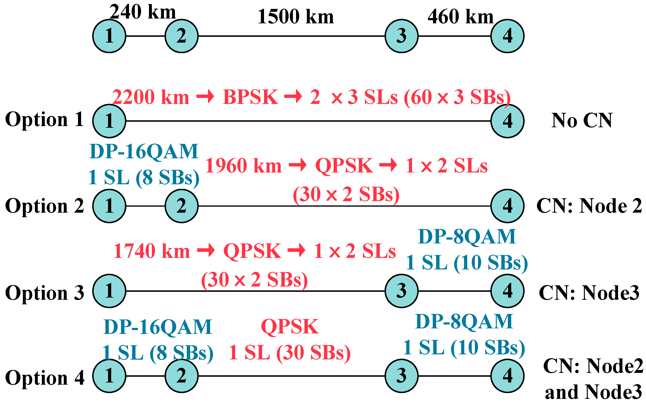
3.3. Modulation Format Conversion

As described in Section 2, the use of MFC to divide the routing path of a traffic request into multiple MFSs can break through the limitation of the longest length segment on spectrum efficiency in traditional optical networks and further achieve efficient utilization of network resources. We assume that MFC is implemented by connecting different transceivers in a back-to-back configuration [54], and the nodes capable of performing MFC are referred to as CNs. Different selections of CNs and MFs lead to different results of network resource occupancy, which is illustrated by an example shown in Figure 3. The complexity of deploying transceivers is not considered here, which will be put into a later study. Each traffic request is defined by (source node, destination node, and traffic rate). In Figure 3, suppose the distances between nodes 1, 2, 3, and 4 are 240 km, 1500 km, and 460 km, respectively. The source and destination nodes of traffic request A (1, 4, 6) are node 1 and node 4, respectively. The traffic rate is 6 Tb/s, and the routing path is 1→2→3→4. Four options to choose CNs on the routing path are discussed.
  • Option 1: no CN is set between node 1 and node 4, i.e., no MFC is performed on the entire routing path. The MF is selected based on the distance from node 1 to node 4, which is 2200 km in Figure 3. From Table 2, BPSK (supporting 100 Gb/s) should be selected as the MF, so 60 × 3 SBs are required to carry A on all links, implying that 2 × 3 SLs are occupied;
  • Option 2: node 2 is set as the CN, and MFC is performed at node 2. The distance from node 1 to node 2 is 240 km, so DP-16QAM (supporting 800 Gb/s) is used as the MF, occupying 1 SL (8 SBs). QPSK (supporting 200 Gb/s) is selected because the distance from node 2 to node 4 is 1960 km, and 1 SL (30 SBs) is occupied. Therefore, 1 + 1 × 2   SLs ( 8 + 30 × 2 SBs) are required to carry A on the routing path;
  • Option 3: node 3 is set as the CN, and MFC is performed at node 3. The distance from node 1 to node 3 is 1740 km, which determines the selection of QPSK (supporting 200 Gb/s) as MF, so 1 SL (30 SBs) is occupied for carrying A. For the distance of 460 km from node 3 to node 4, the DP-8QAM (supporting 600 Gb/s) is selected and 1 SL (10 SBs) is required on the link. As a result, 1 × 2 + 1   SLs ( 30 × 2 + 10   SBs) on the routing path are occupied in Option 3;
  • Option 4: both node 2 and node 3 are set as CNs, and MFC is available at both nodes. The distance from node 1 to node 2 is 240 km, so DP-16QAM (supporting 800 Gb/s) is selected and 1 SL (8 SBs) is occupied. 1 SL (30 SBs) is occupied when QPSK (supporting 200 Gb/s) is selected according to the distance of 1500 km from node 2 to node 3. Moreover, 1 SL (30 SBs) is occupied on the 460 km link between node 3 and node 4 with the adoption of DP-8QAM (supporting 600 Gb/s). Therefore, there are 1 + 1 + 1 SLs ( 8 + 30 + 10   SBs) occupied on the routing path when both node 2 and node 3 are selected as CNs.
This example illustrates all possible options for setting CNs on the routing path of A. No CN is set in option 1, one of the intermediate nodes on the routing path is set as a CN in option 2 and option 3, and both intermediate nodes on the routing path are set as CNs in option 4. It is worth noting that CNs are set in the last three options to achieve MFC, and 6, 3, 3, and 3 SLs (180, 68, 70, and 48 SBs) are occupied corresponding to these four different options to carry traffic request A. The number of occupied SBs and SLs in option 1 is larger than it is in the other three options, all three options improve network resource utilization to some extent. Since node 2 and node 3 are simultaneously set as CNs in option 4 and the most efficient MF is utilized on each SDM link, so the least amount of spectrum resources is occupied to carry A. In summary, choosing the appropriate MF and setting CNs to perform MFC can effectively reduce the spectrum resources and space resources occupied by traffic requests, thus improving the utilization of network resources.

4. RMSSA Problem Formulation in Spatial Channel Networks

This paper is devoted to solving the RMSSA problem in static SCNs by designing efficient algorithms to select the appropriate MF according to the transmission distance and different traffic rate requirements, so that all traffic requests are transmitted with the least amount of occupied network resources. In the static SCN planning phase, all traffic requests are given. SLs and SBs are allocated to different traffic requests as space and spectrum resources, respectively. Sub-core-selective-switch-based SXC architecture is adopted in this paper, which allows spatially demultiplexing SChs from a common SDM port and multiplexing any of SChs into any output SDM port. However, this architecture does not support spatial channel switching, which means that a traffic request is supposed to occupy SLs with the same index on all SDM links. It is assumed that each SDM link is composed of five 4-core MCFs, i.e., each SDM link contains 20 SLs. Each SL with 4THz of available spectrum resources can be divided into 32 SBs.

4.1. Network Topology

Model the SCN topology as a graph G = ( V , E ) , where V = { v 1 , v 2 , , v | V | } denotes a set of nodes and E = { e 1 , e 2 , , e | E | } denotes a set of unidirectional SDM links. Each SDM link e i = ( v i m , v i m , q i ) is defined by the nodes ( v i m , v i n ) it connects and the link length   q i . The 20 SLs on each SDM link are denoted as L = { l 1 , l 2 , l i , , l 20 } , and 32 SBs on each SL are denoted F = { f 1 , f 2 , , f i , , f 32 } .

4.2. Traffic Request Set

Model a node-to-node traffic request set as T = { t 1 , t 2 , , t | T | } and each traffic request t i T can be represented as a tuple t i = ( s i , d i , r i ) defined by a source node s i V , a destination node d i V , and traffic rate r i R , where R is the traffic rate set. For a traffic request t i , its source node s i and destination node d i ( s i d i ) are randomly and uniformly generated, and the sum of all traffic rates r i in the same set T is a fixed value.

4.3. Routing Path, Conversion Node, and Modulation Format Option

According to Table 2, DP-32QAM, DP-16QAM, DP-8QAM, DP-QPSK, QPSK, and BPSK are used. The k-shortest paths (KSP) algorithm is used to obtain the routing path p ( t i ) to establish an optical connection to carry the traffic request t i . For traffic request t i , there are different options of CNs and MFs O ( t i ) = { o 1 ( t i ) , o 2 ( t i ) , , o | O | ( t i ) } , each of which corresponds to a different set of CNs V c o j ( t i ) ( v 1 c , v 2 c , , v | V | c ) V , s i V c o j ( t i ) , d i V c o j ( t i ) . Different CNs divide p ( t i ) into multiple MFSs, and the set of MFSs is defined as Θ o j ( t i ) ( θ 1 , θ 2 , , θ Θ ) E . Each MFS may contain one or more SDM links, and the length of one MFS is equal to the sum of the contained SDM link lengths q o j , θ m t i = e θ m q . The same MF is used on all SDM links in the same MFS.

4.4. Variables

Variables used are shown in Table 3.

4.5. Constraints

4.5.1. Spatial Lane Continuity

Equation (9) shows that if traffic request t is carried on routing path p ( t ) , then index of all SLs carrying t on p ( t ) are supposed to be the same.
θ Θ ω p , o , θ t , , f × e p ( t ) σ e t , = | Θ | 2     t T ,   Θ o ( t ) = p ( t ) , θ o ( t ) Θ o ( t ) ,   if   ω p , o , θ t , , f = 1

4.5.2. Modulation Format Continuity within the Same Modulation Format Segment

Equation (10) shows that after routing path p ( t ) and option o ( t ) of traffic request t are determined, p ( t ) is divided into multiple MFSs θ o ( t ) . It is required that the same MF is used on all SDM links in the same MFS.
e θ m p , o , e t = m p , o , e t × | θ |   t T ,   Θ o ( t ) = p ( t ) , θ o ( t ) Θ o ( t ) ,   e θ ,   if   ω p , o , θ t , l , f = 1

4.5.3. Spectrum Block Continuity within the Same Modulation Format Segment

Equation (11) shows that after routing path p ( t ) and option o ( t ) of traffic request t are determined, p ( t ) is divided into multiple MFSs θ o ( t ) . The number ζ e t and index of occupied SBs on all SDM links in the same MFS are supposed to be the same.
θ Θ e θ ζ e t = θ Θ | θ | × ( μ ¯ e t , l , f μ e t , l , f + 1 ) t T , Θ o ( t ) = p ( t ) , θ o ( t ) Θ o ( t ) , e θ ,   if   ω p , o , θ t , l , f = 1

4.5.4. Spectrum Block Contiguity

Equation (12) shows that when multiple SBs are assigned to traffic request t , it is necessary to ensure that the indexes of multiple SBs on the same SDM link are contiguous.
i = 1 ζ e t σ e t , l , f = ζ e t   t T ,   θ o ( t ) Θ o ( t ) ,   e θ , if   ω p , o , θ t , l , f = 1

4.5.5. Spectrum Nonoverlap

Equation (12) shows that when multiple SBs are assigned to traffic request t , it is necessary to ensure that the indexes of multiple SBs on the same SDM link are contiguous.
σ e t i , , f + σ e t j , , f = 1 ,   μ ¯ e t j , , f μ e t i , , f | t T e E ζ e t | ( φ r r j + 2 ω p , o , θ t j , , f ω p , o , θ t i , , f ) 1 t i , t j T , Θ o ( t ) = p ( t ) , θ o ( t ) Θ o ( t ) ,   e θ , if       ω p , o , θ t i , , f = 1 , ω p , o , θ t j , , f = 1

4.5.6. Guard-Band

Equation (14) shows that if multiple traffic requests with different nodes are carried on the same SL, then the GB (one SB) is supposed to be set between the different traffic requests.
μ e t j , , f j = μ ¯ e t i , , f i + 1 , σ e t , f = ζ e t i + 1 = 0     t i ,   t j T , if   σ e t i , = σ e t j , = 1  

4.6. Objective Function

Under the above constraints, the objective of accommodating all traffic requests with the minimum number of SLs and SBs is to be achieved.
Minimize :   e E l max ,   Minimize :   t T e E ζ e t .

5. LBMSA Algorithm

Since the RMSA problem is part of the RMSSA problem and the RMSA problem is NP-hard, the RMSSA problem is also NP-hard. To solve the RMSSA problem, we proposed a heuristic algorithm called spatial lane and spectrum block minimization based on the simulated annealing (LBMSA) algorithm, as shown in Algorithms 1 and 2.
First, the LBMSA algorithm classifies all traffic requests with the same source and destination nodes (link directional) into the same set T ¯ s , d (Algorithm 1: lines 1–3). The traffic rate r of all traffic requests in each T ¯ s , d are summed to obtain t T ¯ s , d r , and all T ¯ s , d are sorted in descending order according to t T ¯ s , d r (Algorithm 1: lines 4–6). The RMSSA is performed one by one starting from the T ¯ s , d with the max ( t T ¯ s , d r ) value and the specific allocation method is the same in different T ¯ s , d . Once the RMSSA of all traffic requests in a T ¯ s , d has been finished, the RMSSA for the next T ¯ s , d is carried out (Algorithm 1: lines 7–29). When performing RMSSA in each T ¯ s , d , all traffic requests in that T ¯ s , d are first randomly ordered, and each traffic request is assigned in that order in turn (Algorithm 1: line 8). The SA algorithm is then used to optimize the order of traffic requests in T ¯ s , d . The order of traffic requests is adjusted by iterations so that the objective function value is minimized while all traffic requests in T ¯ s , d are carried on the network (Algorithm 1: lines 12–23).
The process of performing RMSSA in each T ¯ s , d is as follows. Following the random ordering of the traffic requests in T ¯ s , d , the network resource allocation scheme X 0 ( Λ , Ω ) under that order and the corresponding fitness value f ( X 0 )   are obtained, which are used as the initial parameter values for the SA optimization process (Algorithm 1: lines 9–10). Following the reordering the traffic requests using the SA algorithm, Algorithm 2 is used to allocate space resources and spectrum resources to each traffic request in turn. The KSP algorithm is used to find the shortest routing path for each traffic request and calculate all possible options for CNs and MFs on that routing path (Algorithm 2: lines 2–3). Calculate the number of SLs and SBs that will be occupied corresponding to the different options and select the option that minimizes e E l max over the entire network (Algorithm 2: lines 4–7). Select the option with the smallest t T e E ζ e t when the e E l max of different options are equal (Algorithm 2: lines 8–9). First-fit (FF) policy is used to assign SLs and SBs to a traffic request. In other words, starting from the SL with the smallest index, the unoccupied network resources that can carry the traffic request are searched in the order of SB index from smallest to largest.
The following two points should be noted. First, when traffic requests in different T ¯ s , d are carried on the same SL, the GB (one SB) is supposed to be set between these traffic requests. Second, all traffic requests are classified according to whether the nodes are the same so that traffic requests are transmitted by the Type I SCh or Type Ⅱ SCh as much as possible, which reduces the use of WXCs and thus the switching cost.
The time complexity of the LBMSA algorithm is related to the SA algorithm. Let the initial temperature of the SA algorithm be T 0 , the cooling rate be β, the end temperature be T e , and there is T e = ( 1 β ) k T 0 . The SA algorithm terminates at k > ln Δ T 0 ln β . Where Δ represents the difference in order of magnitude between the end temperature and the initial temperature. Then the number of external loops of the temperature control is M = ln Δ T 0 ln β + 1 . For the objective function of the SA algorithm, the time complexity of the whole algorithm is O ( M × N × n )   when the number of internal cycles is N at each specific temperature.
Algorithm 1 Traffic Request Order Optimization with SA
Input:  Network   topology G = ( V , E ) , traffic request set T = { t 1 , t 2 , , t | T | } ,   t i = ( s i , d i , r i )
Output:  f ( X b e s t )
1: for  t T  do
2:    Classify different traffic requests
3:     t i T ¯ s i , d i ,   t j T ¯ s j , d j { s i = s j d i = d j or { s i = d j d i = s j
4:    for  T ¯ s , d  do
5:      t T ¯ s , d r sum { r i   of   ( t i T ¯ s , d ) }
6:      T = { T ¯ s 1 , d 1 , T ¯ s 2 , d 2 , , T ¯ s M , d M } sort   T b y t T ¯ s , d r   from   large   to   small
7:     for  q = 1 : M  do
8:       T ¯ s , d = { t 1 , t 2 , , t | T ¯ s , d | }   sort T ¯ s , d randomly
9:      Generate a solution X 0 ( Λ , Ω )
10:    Calculate fitness value f ( X 0 )   Algorithm 2
11:     X b e s t X 0 , k 0 , t k T
12:     if  t k + 1 < t h r e s h o l d  then
13:       for i = 1 : L  do
14:       swap two randomly selected traffic requests
15:        X n e w ( Λ n e w , Ω n e w ) , f ( X n e w )   Algorithm 2
16:          if  f ( X n e w )   <   f ( X k )   then
17:           X k = X n e w  
18:          if  f ( X k )   <   f ( ( X b e s t ) X b e s t = X k )   then
19:            continue
20:          end if
21:          end if
22:         P ( t k ) = e [ f ( X n e w ) f ( X k ) t k ]     calculate
23:         X k = X n e w     random ( 0 , 1 ) < P
24:       end for
25:        t k + 1     drop ( t k )
26:        k = k + 1
27:      end if
28:    end for
29:  end for
30: end for
Algorithm 2 SLs and SBs Assignment
Input:   T ¯ s , d = { t 1 , t 2 , , t | T ¯ s , d | } , G
Output:   e E l max ,   t T e E ζ e t
1: for  i = 1 len ( T ¯ s , d )   do
2:   p ( t i )   finding   routing   path   using   KSP
3:   O ( t i ) = { o 1 ( t i ) , o 2 ( t i ) , , o | O ( t i ) | ( t i ) }   finding   all   CNs   &   MFs   on   p ( t i )
4:  for  j = 1 , 2 , , | O ( t i ) |   do
5:     e E , o j ( t i ) l max     calculate   the   number   of   occupied   SLs   in   the   whole   network
6:      t T e E , o j ( t i ) ζ e t   calculate   the   number   of   occupied   SBs   in   the   whole   network
7:  end for
8:   o b e s t ( t i ) { min ( e E , o j ( t i ) l max )   and   min ( t T e E , o j ( t i ) ζ e t ) }
9:   Λ = e E , o b e s t ( t i ) l max ,   Ω = t T e E , o b e s t ( t i ) ζ e t o b e s t ( t i )
10: end for

6. Simulation Results

In order to verify the effectiveness of the LBMSA algorithm, we performed simulations on MATLAB and analyzed the simulation results.

6.1. Simulation Settings

We evaluated the performance of the proposed algorithms in the simple mesh network topology, the Japan network topology, and the NSF network topology using MATLAB. The characteristics of the three network topologies are shown in Figure 4 and Table 4. We simulated the SCN based on the sub-core-selective-switch-based SXC architecture, which does not support spatial channel switching. Each SDM link consists of five 4-core MCFs, i.e., one SDM link contains 20 SLs, and each SL is divided into 32 SBs. Then, 112-Gbaud transceivers are deployed in the whole network without considering the complexity and cost, which transmit/receive an OCh that occupies 125 GHz. The bit rate and transmission distance that can be supported by each transceiver using different MFs are shown in Table 2. Suppose four traffic request sets are generated, each with 50 traffic requests of possible traffic rates of 2 Tb/s, 4 Tb/s, 6 Tb/s, 8 Tb/s, and 10 Tb/s. The source and destination nodes of each traffic request are randomly and uniformly generated and the sum of the traffic rates in the four sets is 200 Tb/s, 250 Tb/s, 300 Tb/s, and 350 Tb/s, respectively. The LBMSA algorithm and its comparison algorithms are used to allocate network resources to traffic request sets in different networks, and the occupancy of spatial and spectral resources in the corresponding cases is analyzed. The usage of MF and MFC when applying the LBMSA algorithm for resource allocation is also analyzed. To further demonstrate the effectiveness of the LBMSA algorithm, we also tested the maximum sum of traffic request rates that the three networks can carry, and analyzed the results.
To illustrate the importance of MF and MFC in the resource allocation of static SCNs, we compare the proposed LBMSA algorithm with the KSP algorithm and the KSP-CNs (KSP with CNs) algorithm. CNs and MFC are not considered in the KSP algorithm. That is, no CN is set on the routing path, the MF is selected based on the total length of all SDM links contained in the routing path, and the same MF is used for the whole connection. MFC is not considered in the KSP-CNs algorithm. Similar to the LBMSA algorithm, after determining the routing path for a traffic request, the KSP-CNs algorithm calculates all possible options of CNs and MFs on that routing path. However, CNs do not perform MFC, but only determine one MF to be applied to the whole routing path based on the length of the longest MFS. We use network resource utilization as a metric to evaluate these algorithms.

6.2. Simulation Results Analysis

First, the network resources that would be occupied by applying three different algorithms to carry the same traffic requests are analyzed in Figure 5. The traffic rate sum of 50 traffic requests is set to 200 Tb/s. In the simple mesh network topology, 69 SLs (1792 SBs) are occupied when the LBMSA algorithm is applied to carry all traffic requests, 123 SLs (3235 SBs) are occupied when the KSP algorithm is applied, and 123 SLs (3115 SBs) are occupied when KSP-CNs algorithm is applied. In the Japan network topology, 58 SLs (1257 SBs), 99 SLs (2394 SBs), and 105 SLs (2382 SBs) are occupied by applying the LBMSA algorithm, KSP algorithm, and the KSP-CNs algorithm, respectively. Moreover, in the NSF network topology, the occupied network resources are 135 SLs (3610 SBs), 170 SLs (4495 SBs), and 170 SLs (4495 SBs) by applying the LBMSA algorithm, KSP, and KSP-CNs algorithm, respectively. It can be seen that by using the LBMSA algorithm, as few SLs and SBs as possible are occupied to carry the traffic requests. When simulating the simple mesh network topology and the Japan network topology, using the LBMSA algorithm saves almost half of the network resources, compared to the latter two algorithms. Furthermore, in the NSF network topology, using the LBMSA algorithm also saves about 20% of SLs and SBs, compared to the latter two algorithms. The above simulation results show that the LBMSA algorithm can allocate the least amount of network resources to carry the traffic requests by setting CNs and performing MFC. In addition, in Figure 5, the NSF network topology with the largest average SDM link length occupies more network resources because the less efficient MFs are used.
The simulation results of the KSP algorithm and the KSP-CNs algorithm are analyzed and compared in Figure 5. In the simple mesh network topology, the same number of SLs are assigned to the traffic requests using both algorithms, but the number of occupied SBs using the KSP algorithm is 4% more than that using the KSP-CNs algorithm. This is because the KSP-CNs algorithm saves spectrum resources by setting CNs, dividing routing paths into shorter-length MFSs, and selecting more efficient MFs. In the Japan network topology, there is little difference in the number of network resources used to carry the traffic requests using the two algorithms, due to the large variance in SDM link lengths. Applying the MF of the longest MFS to the entire routing path does not necessarily reduce the occupied network resources and may have the opposite effect. In the NSF network topology, although the optimization results of both algorithms are the same, the indexes and numbers of SLs and SBs assigned to the same traffic request are not the same because SA is used to optimize the sum of the network resources occupied by all traffic requests.
In Figure 6, the occupancy of SLs and SBs using the three algorithms is analyzed under different traffic loads. Different traffic request sets are constructed by varying the traffic rate without changing the number of traffic requests inside each set. When the LBMSA algorithm is used, the number of SLs and SBs occupied in the three networks is increased as the traffic load increases, except for one special case. This special case was found when the simulation data of the NSF network topology was analyzed. Theoretically, the number of SLs and SBs assigned to the traffic request set of 350 Tb/s should be the maximum. However, when the total traffic rate is 350 Tb/s, the number of occupied SLs and SBs is 161 and 4489, respectively, which is less than the number of occupied SLs and SBs when the total traffic rate is 250 Tb/s and 300 Tb/s. The reason for the special case is that, in the same T ¯ s , d , after the allocation of traffic requests that occupy more SBs, the remaining spectrum resources in each SL happen to carry the traffic requests that occupy fewer SBs. Therefore, the number of occupied SLs is reduced instead. To verify the specificity of this case, three other different 350 Tb/s traffic request sets were generated for simulation. The simulation results are consistent with the theoretical analysis, i.e., the number of SLs and SBs allocated to the 350 Tb/s traffic request set is the maximum.
As shown in Figure 6, LBMSA clearly occupies fewer SLs and SBs than the other two algorithms and can save more network resources, which also means that using the LBMSA algorithm can make SCNs have greater throughput. Comparing the KSP algorithm with the KSP-CNs algorithm, the number of SLs and SBs occupied using the KSP-CNs algorithm is slightly smaller than the number in the KSP algorithm. This shows that even without MFC, segmenting the entire routing path and using a flexible MF is effective. Comparing the LBMSA algorithm with the KSP-CNs algorithm, there is a significant difference in the amount of network resources occupied by the two algorithms because LBMSA can perform MFC at the CNs. This illustrates the importance of introducing MFC into SCNs in this paper.
In Figure 7 and Figure 8, the utilization of MFs and MFC in three network topologies is analyzed. We obtained the number of traffic requests that were not end-to-end requests under different traffic load scenarios and calculated the percentage of those traffic requests that performed MFC. It can be obtained that the adoption of different MFs and MFC is related to the average SDM link length of the network topology and the use of MFC is also related to the total traffic rate. In the simple mesh network topology, QPSK and DP-QPSK (with maximum achievable transmission distances of 1000 km and 2000 km, respectively) are used most frequently because of the average SDM link length of 1063 km and the small SDM link length variance. As a result, in Figure 8, multiple CNs are set up to perform MFC to carry traffic requests using more efficient MFs. When the total traffic rate is 200 Tb/s, the percentage of traffic requests performing MFC even reaches 85%. This also proves that when the traffic attempt rate in the network is small, the LBMSA algorithm takes maximizing network resource utilization as the primary goal. Since the average SDM link length of the Japan network topology is small, more efficient MFs, such as DP-8QAM, DP-16QAM, and DP-32QAM are effectively utilized. Meanwhile, the SDM link length variance in the Japan network topology is large, so CNs and MFC are used more frequently than in the simple mesh network topology. This is why the number of SLs and SBs occupying the Japan network topology is always less than that of a simple mesh network when the traffic rates are the same. The average SDM link length in the NSF network topology is 1936.36 km, therefore, the inefficient BPSK and QPSK are used many times, which is consistent with the analysis above. LBMSA always saves more network resources, compared to the other two algorithms and is particularly prominent in small-scale networks. When the size of the network is small, insufficient spectrum resources are the only reason for blocking. In addition, as can be seen in Figure 8, the percentage of traffic requests using MFC is above 75% for different traffic load cases. The high frequency of using MFC is also an important reason for the efficiency of LBMSA. The use of MFC tends to decrease as the traffic load increases. In all three network topologies, the use of MFC is minimal when the total traffic rate is 350 Tb/s. This is because when the network traffic load increases, the LBMSA algorithm is more inclined to carry all traffic requests rather than efficient transmission.

7. Conclusions

This paper was dedicated to solving the network resource allocation problem in static SCNs. First, the network resource allocation problem in SCNs was defined as the RMSSA problem. Flexible MFs for SCNs were studied and MFC is applied for the first time to solve the RMSSA problem. Then, the RMSSA problem in static SCNs was modeled and the heuristic LBMSA algorithm was proposed to solve the RMSSA problem. Finally, the LBMSA was evaluated in three different network topologies and both the KSP algorithm and the KSP-CNs algorithm were used to compare with the LBMSA algorithm to demonstrate the effectiveness of the algorithm. The simulation results show that when the total throughput of SCNs is less than 350 Tb/s, the LBMSA algorithm can traffic requests with the least amount of SBs. When the total network throughput is larger, it is not always possible to maximize network resource utilization. This is because the LBMSA algorithm prefers to carry all traffic requests rather than efficiently transmit them. Moreover, by reasonably setting CNs to execute MFC, the LBMSA algorithm will select the optimal MF option. This not only effectively solves the RMSSA problem, but also saves at least 20% of the network resources, further improving the network resource utilization. However, this paper still has some limitations. In this paper, the complexity and the economic costs of deploying transceivers, as well as the tradeoff between spectrum block, SLs, and transceiver utilization, have not been considered. In addition, this paper only studies the resource allocation problem in static SCNs, and only considers reducing the resource occupation of traffic requests and improving network resource utilization. The more complex problem of resource allocation in dynamic SCNs, which is dedicated to reducing traffic request blocking rate, will be investigated in our future work.

Author Contributions

Conceptualization, methodology, formal analysis, investigation, data curation, writing—original draft preparation, writing—review and editing, X.Y.; software, validation, X.Y. and Y.Z.; supervision, project administration, Q.S. All authors have read and agreed to the published version of the manuscript.

Funding

This research received no external funding.

Institutional Review Board Statement

Not applicable.

Informed Consent Statement

Not applicable.

Data Availability Statement

Data available upon request. The data presented in this study are available on request from the corresponding author. The data are not publicly available due to our further study on these data is needed.

Conflicts of Interest

The authors declare no conflict of interest.

References

  1. Winzer, P.J.; Neilson, D.T. From Scaling Disparities to Integrated Parallelism: A Decathlon for a Decade. J. Light. Technol. 2017, 35, 1099–1115. [Google Scholar] [CrossRef]
  2. Jinno, M.; Takara, H.; Kozicki, B.; Tsukishima, Y.; Sone, Y.; Matsuoka, S. Spectrum-efficient and scalable elastic optical path network: Architecture, benefits, and enabling technologies. IEEE Commun. Mag. 2009, 47, 66–73. [Google Scholar] [CrossRef]
  3. Jinno, M.; Takara, H.; Kozicki, B.; Tsukishima, Y.; Sone, Y.; Matsuoka, S. Demonstration of novel spectrum-efficient elastic optical path network with per-channel variable capacity of 40 Gb/s to over 400 Gb/s. In Proceedings of the 34th ECOC 2008 34th European Conference on Optical Communication, Brussels, Belgium, 21–25 September 2008; pp. 1–2. [Google Scholar] [CrossRef]
  4. Jinno, M.; Ohara, T.; Sone, Y.; Hirano, A.; Ishida, O.; Tomizawa, M. Elastic and adaptive optical networks: Possible adoption scenarios and future standardization aspects. IEEE Commun. Mag. 2011, 49, 164–172. [Google Scholar] [CrossRef]
  5. Gerstel, O.; Jinno, M.; Lord, A.; Yoo, S.J.B. Elastic optical networking: A new dawn for the optical layer? IEEE Commun. Mag. 2012, 50, s12–s20. [Google Scholar] [CrossRef]
  6. Jinno, M. Spatial Channel Network (SCN) Architecture Employing Growable and Reliable Spatial Channel Cross-Connects Toward Massive SDM Era. In Proceedings of the 2018 Int. Conf. PSC Photonics in Switching and Computing, Limassol, Cyprus, 19–21 September 2018; pp. 1–3. [Google Scholar] [CrossRef]
  7. Hashimoto, R.; Yamaoka, S.; Mori, Y.; Hasegawa, H.; Sato, K.-I.; Yamaguchi, K.; Seno, K.; Suzuki, K. First Demonstration of Subsystem-Modular Optical Cross-Connect Using Single-Module 6 × 6 Wavelength-Selective Switch. J. Light. Technol. 2018, 36, 1435–1442. [Google Scholar] [CrossRef]
  8. Winzer, P.J. Spatial multiplexing: The next frontier in network capacity scaling. In Proceedings of the 39th ECOC 2013 European Conference and Exhibition on Optical Communication, London, UK, 22–26 September 2013; pp. 1–4. [Google Scholar] [CrossRef]
  9. Jinno, M.; Yamashita, K.; Asano, Y. Architecture and Feasibility Demonstration of Core Selective Switch (CSS) for Spatial Channel Network (SCN). In Proceedings of the 2019 24th OptoElectronics and Communications Conference (OECC) and 2019 International Conference on Photonics in Switching and Computing (PSC), Fukuoka, Japan, 7–11 July 2019; pp. 1–3. [Google Scholar] [CrossRef]
  10. Jinno, M. Opportunities, Challenges, and Solutions for Spatial Channel Networks (SCNs) Toward the SDM Abundant Era. In Proceedings of the 2019 24th OptoElectronics and Communications Conference (OECC) and 2019 International Conference on Photonics in Switching and Computing (PSC), Fukuoka, Japan, 7–11 July 2019; pp. 1–3. [Google Scholar] [CrossRef]
  11. Jinno, M.; Asano, Y. Required Link and Node Resource Comparison in Spatial Channel Networks (SCNs) Employing Modular Spatial Channel Cross-Connects (SXCs). In Proceedings of the 2019 OFC Optical Fiber Communication Conference, San Diego, CA, USA, 3–7 March 2019; pp. 1–3. [Google Scholar]
  12. Jinno, M. Spatial Channel Network (SCN): Opportunities and Challenges of Introducing Spatial Bypass Toward the Massive SDM Era. J. Opt. Commun. Netw. 2019, 11, 1–14. [Google Scholar] [CrossRef]
  13. Jinno, M. Benefits of Hierarchical Spatial Bypassing and Spectral Grooming in Spatial Channel Networks. In Proceedings of the 2020 ECOC European Conference on Optical Communication, Brussels, Belgium, 6–10 December 2020; pp. 1–4. [Google Scholar] [CrossRef]
  14. Jinno, M.; Kodama, T.; Ishikawa, T. Feasibility Demonstration of Spatial Channel Networking Using SDM/WDM Hierarchical Approach for Peta-b/s Optical Transport. J. Light. Technol. 2020, 8, 2577–2586. [Google Scholar] [CrossRef]
  15. Jinno, M.; Kodama, T. Spatial Channel Network (SCN): Introducing Spatial Bypass Toward the SDM Era. In Proceedings of the 2020 OFC Optical Fiber Communication Conference, San Diego, CA, USA, 8–12 March 2020. [Google Scholar]
  16. Jinno, M.; Ishikawa, T.; Kodama, T.; Hasegawa, H.; Subramaniam, S. Enhancing the flexibility and functionality of SCNs: Demonstration of evolution toward any-core-access, nondirectional, and contentionless spatial channel cross-connects. J. Opt. Commun. Netw. 2021, 13, D80–D92. [Google Scholar] [CrossRef]
  17. Jinno, M.; Takara, H.; Kozicki, B. Concept and enabling technologies of spectrum-sliced elastic optical path network (SLICE). In Proceedings of the 2009 ACP Asia Communications and Photonics Conference and Exhibition, Shanghai, China, 2–6 November 2009; pp. 1–2. [Google Scholar] [CrossRef]
  18. Zhao, Y.; Zhang, J.; Ji, Y.; Gu, W. Routing and Wavelength Assignment Problem in PCE-Based Wavelength-Switched Optical Networks. J. Opt. Commun. Netw. 2010, 2, 196–205. [Google Scholar] [CrossRef]
  19. Jia, X.; Ning, F.; Yin, S.; Wang, D.; Zhang, J.; Huang, S. An integrated ILP model for Routing, Modulation Level and Spectrum Allocation in the next generation DCN. In Proceedings of the 3rd Int. Conf. CCT 2015 Third International Conference on Cyberspace Technology, Beijing, China, 17–18 October 2015; pp. 1–3. [Google Scholar] [CrossRef]
  20. Enoch, J.; Jaumard, B. Towards Optimal and Scalable Solution for Routing and Spectrum Allocation. Electron. Notes Discret. Math. 2018, 64, 335–344. [Google Scholar] [CrossRef]
  21. Goscień, R.; Walkowiak, K.; Klinkowski, M. Tabu search algorithm for routing, modulation and spectrum allocation in elastic optical network with anycast and unicast traffic. Comput. Netw. 2015, 79, 148–165. [Google Scholar] [CrossRef]
  22. Goścień, R. Two metaheuristics for routing and spectrum allocation in cloud-ready survivable elastic optical networks. Swarm Evol. Comput. 2019, 44, 388–403. [Google Scholar] [CrossRef]
  23. Lezama, F.; Castañón, G.; Sarmiento, A.M.; Martins, I.B. Routing and spectrum allocation in flexgrid optical networks using differential evolution optimization. In Proceedings of the 2014 16th ICTON International Conference on Transparent Optical Networks, Graz, Austria, 6–10 July 2014; pp. 1–4. [Google Scholar] [CrossRef]
  24. Nagły, P.; Walkowiak, K. Simulated Annealing Algorithm for Minimization of Bandwidth Fragmentation in Elastic Optical Networks with Multicast and Unicast Flows. In Proceedings of the IDEAL 2015 Intelligent Data Engineering and Automated Learning–IDEAL 2015: 16th International Conference, Wroclaw, Poland, 14–16 October 2015; pp. 318–327. [Google Scholar] [CrossRef]
  25. Marković, G.Z. Routing and spectrum allocation in elastic optical networks using bee colony optimization. Photonic Netw. Commun. 2017, 34, 356–374. [Google Scholar] [CrossRef]
  26. Yuan, J.; Fu, Y.; Zhu, R.; Li, X.; Zhang, Q.; Zhang, J.; Samuel, A. A constrained-lower-indexed-block spectrum assignment policy in elastic optical networks. Opt. Switch. Netw. 2019, 33, 25–33. [Google Scholar] [CrossRef]
  27. Munasinghe, K.K.; Dharmaweera, M.N.; Wijewardhana, U.L.; De Alwis, C.; Parthiban, R. Joint Minimization of Spectrum and Power in Impairment-Aware Elastic Optical Networks. IEEE Access 2021, 9, 43349–43363. [Google Scholar] [CrossRef]
  28. Jia, W.; Xu, Z.; Ding, Z.; Wang, K. An Efficient Routing and Spectrum Assignment Algorithm Using Prediction for Elastic Optical Networks. In Proceedings of the 2016 Int. Conf. ISAI International Conference on Information System and Artificial Intelligence, Hong Kong, China, 24–26 June 2016; pp. 89–93. [Google Scholar] [CrossRef]
  29. Yang, H.; Bai, W.; He, L.; Xiao, H.; Zhang, J. Leveraging Deep Learning to Achieve Efficient Resource Allocation with Traffic Evaluation in Datacenter Optical Networks. In Proceedings of the 2018 OFC Optical Fiber Communications Conference and Exposition, San Diego, CA, USA, 11–15 March 2018; pp. 1–3. [Google Scholar]
  30. Chen, X.; Li, B.; Proietti, R.; Lu, H.; Zhu, Z.; Yoo, S.J.B. DeepRMSA: A Deep Reinforcement Learning Framework for Routing, Modulation and Spectrum Assignment in Elastic Optical Networks. J. Light. Technol. 2019, 37, 4155–4163. [Google Scholar] [CrossRef]
  31. Muhammad, A.; Zervas, G.; Simeonidou, D.; Forchheimer, R. Routing, spectrum and core allocation in flexgrid SDM networks with multi-core fibers. In Proceedings of the 2014 Int. Conf. ONDM International Conference on Optical Network Design and Modeling, Stockholm, Sweden, 19–22 May 2014; pp. 192–197. [Google Scholar]
  32. Rumipamba-Zambrano, R.; Moreno-Muro, F.J.; Pavón-Marino, P.; Perelló, J.; Spadaro, S.; Solé-Pareta, J. Assessment of Flex-Grid/MCF Optical Networks with ROADM limited core switching capability. In Proceedings of the 2017 Int. Conf. ONDM International Conference on Optical Network Design and Modeling, Budapest, Hungary, 15–18 May 2017; pp. 1–6. [Google Scholar] [CrossRef]
  33. Moreno-Muro, F.; Rumipamba-Zambrano, R.; Pavón-Marino, P.; Perelló, J.; Gené, J.M.; Spadaro, S. Evaluation of core-continuity-constrained ROADMs for flex-grid/MCF optical networks. J. Opt. Commun. Netw. 2017, 9, 1041–1050. [Google Scholar] [CrossRef]
  34. Yang, M.; Zhang, Y.; Wu, Q. Routing, spectrum, and core assignment in SDM-EONS with MCF: Node-arc ILP/MILP methods and an efficient XT-aware heuristic algorithm. J. Opt. Commun. Netw. 2018, 10, 195–208. [Google Scholar] [CrossRef]
  35. Yousefi, F.; Rahbar, A.G.; Ghadesi, A. Fragmentation and time aware algorithms in spectrum and spatial assignment for space division multiplexed elastic optical networks (SDM-EON). Comput. Netw. 2020, 174, 107232. [Google Scholar] [CrossRef]
  36. Halder, J.; Acharya, T.; Bhattacharya, U. A Novel RSCA Scheme for offline Survivable SDM-EON with Advance Reservation. IEEE Trans. Netw. Serv. Manag. 2022, 19, 804–817. [Google Scholar] [CrossRef]
  37. Jinno, M.; Kozicki, B.; Takara, H.; Watanabe, A.; Sone, Y.; Tanaka, T.; Hirano, A. Distance-adaptive spectrum resource allocation in spectrum-sliced elastic optical path network [Topics in Optical Communications]. IEEE Commun. Mag. 2010, 48, 138–145. [Google Scholar] [CrossRef]
  38. Klinkowski, M.; Ksieniewicz, P.; Jaworski, M.; Zalewski, G.; Walkowiak, K. Machine Learning Assisted Optimization of Dynamic Crosstalk-Aware Spectrally-Spatially Flexible Optical Networks. J. Light. Technol. 2020, 38, 1625–1635. [Google Scholar] [CrossRef]
  39. Morales, P.; Lozada, A.; Borquez-Paredes, D.; Olivares, R.; Saavedra, G.; Leiva, A.; Beghelli, A.; Jara, N. Improving the Performance of SDM-EON Through Demand Prioritization: A Comprehensive Analysis. IEEE Access 2021, 9, 63475–63490. [Google Scholar] [CrossRef]
  40. Jinno, M.; Yonenaga, K.; Takara, H.; Shibahara, K.; Yamanaka, S.; Ono, T.; Kawai, T.; Tomizawa, M.; Miyamoto, Y. Demonstration of translucent elastic optical network based on virtualized elastic regenerator. In Proceedings of the OFC/NFOEC National Fiber Optic Engineers Conference, Los Angeles, CA, USA, 4–8 March 2012; pp. 1–3. [Google Scholar]
  41. Simmons, J.M. Routing Algorithms. In Optical Network Design and Planning; Springer US: New York, NY, USA, 2008; pp. 61–97. [Google Scholar]
  42. Cerutti, I.; Martinelli, F.; Sambo, N.; Cugini, F.; Castoldi, P. Trading Regeneration and Spectrum Utilization in Code-Rate Adaptive Flexi-Grid Networks. J. Light. Technol. 2014, 32, 4496–4503. [Google Scholar] [CrossRef]
  43. Klinkowski, M.; Walkowiak, K. A heuristic algorithm for routing, spectrum, transceiver and regeneration allocation problem in elastic optical networks. In Proceedings of the 2016 18th ICTON International Conference on Transparent Optical Networks, Trento, Italy, 10–14 July 2016; pp. 1–4. [Google Scholar] [CrossRef]
  44. Klinkowski, M.; Walkowiak, K. On Performance Gains of Flexible Regeneration and Modulation Conversion in Translucent Elastic Optical Networks with Superchannel Transmission. J. Light. Technol. 2016, 34, 5485–5495. [Google Scholar] [CrossRef]
  45. Klinkowski, M.; Walkowiak, K. Performance analysis of flexible regeneration and modulation conversion in elastic optical networks. In Proceedings of the 2017 OFC Optical Fiber Communication Conference, Los Angeles, CA, USA, 19–23 March 2017; pp. 1–3. [Google Scholar]
  46. Walkowiak, K.; Klinkowski, M.; Lechowicz, P. Scalability Analysis of Spectrally-Spatially Flexible Optical Networks with Back-to-Back Regeneration. In Proceedings of the 2018 20th ICTON International Conference on Transparent Optical Networks, Bucharest, Romania, 1–5 July 2018; pp. 1–4. [Google Scholar] [CrossRef]
  47. Walkowiak, K.; Klinkowski, M.; Lechowicz, P. Dynamic routing in spectrally spatially flexible optical networks with back-to-back regeneration. J. Opt. Commun. Netw. 2018, 10, 523–534. [Google Scholar] [CrossRef]
  48. Jinno, M.; Asano, Y.; Azuma, Y.; Kodama, T.; Nakai, R. Technoeconomic analysis of spatial channel networks (SCNs): Benefits from spatial bypass and spectral grooming. J. Opt. Commun. Netw. 2021, 13, A124–A134. [Google Scholar] [CrossRef]
  49. Yang, M.; Wu, Q.; Shigeno, M.; Zhang, Y. Hierarchical Routing and Resource Assignment in Spatial Channel Networks (SCNs): Oriented Toward the Massive SDM Era. J. Light. Technol. 2021, 39, 1255–1270. [Google Scholar] [CrossRef]
  50. Mitra, P.; Stark, J. Nonlinear Limits to the Information Capacity of Optical Fibre Communications. Nature 2001, 411, 1027–1030. [Google Scholar] [CrossRef]
  51. Xu, J.; Yu, J.; Hu, Q.; Li, M.; Liu, J.; Luo, Q.; Huang, L.; Luo, J.; Zhou, H.; Zhang, L.; et al. 50G BPSK, 100G SP-QPSK, 200G 8QAM, 400G 64QAM Ultra Long Single Span Unrepeatered Transmission over 670.64 km, 653.35 km, 601.93 km and 502.13 km Respectively. In Proceedings of the Optical Fiber Communication Conference (OFC) 2019, San Diego, CA, USA, 3–7 March 2019; pp. 1–3. [Google Scholar]
  52. Carena, A.; Curri, V.; Bosco, G.; Poggiolini, P.; Forghieri, F. Modeling of the Impact of Nonlinear Propagation Effects in Uncompensated Optical Coherent Transmission Links. J. Light. Technol. 2012, 30, 1524–1539. [Google Scholar] [CrossRef]
  53. Bosco, G.; Curri, V.; Carena, A.; Poggiolini, P.; Forghieri, F. On the Performance of Nyquist-WDM Terabit Superchannels Based on PM-BPSK, PM-QPSK, PM-8QAM or PM-16QAM Subcarriers. J. Light. Technol. 2011, 29, 53–61. [Google Scholar] [CrossRef]
  54. Eira, A.; Santos, J.; Pedro, J.; Pires, J. Multi-objective design of survivable flexible-grid DWDM networks. J. Opt. Commun. Netw. 2014, 6, 326–339. [Google Scholar] [CrossRef]
Figure 1. Spatial channel network (SCN) model.
Applsci 13 02105 g001
Figure 2. Example of flexible MF cases for provisioning 2 Tb/s traffic requests on routing path 1→2→3.
Applsci 13 02105 g002
Figure 3. Example of different MF options for provisioning 6 Tb/s traffic requests on routing path 1→2→3→4.
Applsci 13 02105 g003
Figure 4. (a) Simple mesh network topology; (b) Japan network topology; (c) NSF network topology.
Applsci 13 02105 g004
Figure 5. (a) The number of occupied SLs and SBs for the LBMSA algorithm, the KSP algorithm, and the KSP-CNs algorithm in the simple mesh network; (b) The number of occupied SLs and SBs for the LBMSA algorithm, the KSP algorithm, and the KSP-CNs algorithm in the Japan network; (c) The number of occupied SLs and SBs for the LBMSA algorithm, the KSP algorithm, and the KSP-CNs algorithm in the NSF network.
Applsci 13 02105 g005
Figure 6. (a) The number of occupied SLs and SBs for the different traffic loads in the simple mesh network; (b) The number of occupied SLs and SBs for different traffic loads in the Japan network; (c) The number of occupied SLs and SBs for different traffic loads in the NSF network.
Applsci 13 02105 g006
Figure 7. (a) Utilization of the modulation formats in the simple mesh network; (b) Utilization of the modulation formats in the Japan network; (c) Utilization of the modulation formats in the NSF network.
Applsci 13 02105 g007
Figure 8. Percentage of traffic requests performing MFC.
Applsci 13 02105 g008
Table 2. Supported traffic rate and maximum transmission distance under different modulation formats using a 125 GHz spectrum block.
Modulation FormatSupported Traffic Rate (Gb/s)Achievable Transmission Distance (km)
BPSK1004000
QPSK2002000
DP-QPSK4001000
DP-8QAM600500
DP-16QAM800250
DP-32QAM1000125
Table 3. Variable table.
VariableConditionValue
ω p , o , θ t , l , f Traffic request t is carried on routing path p ( t ) adopting option   o ( t ) , SL l , and SB f of MFS θ is assigned to t 1
Otherwise0
m p , o , e θ t 0 < q o , θ t 125   km 0 → (DP-32QAM)
125   km < q o , θ t 250   km 1 → (DP-16QAM)
250   km < q o , θ t 500   km 2 → (DP-8QAM)
500   km < q o , θ t 1000   km 3 → (DP-QPSK)
1000   km < q o , θ t 2000   km 4 → (QPSK)
2000   km < q o , θ t 4000   km 5 → (BPSK)
σ e t , l SL l on SDM link e is assigned to t 1
Otherwise0
σ e t , l , f SB f on SL l on SDM link e is assigned to t 1
Otherwise0
φ i j μ ¯ e t j , l , f > μ e t i , l , f . μ e t , l , f is the index of the starting SB on SDM link e ,   μ ¯ e t , l , f is the index of the ending SB on SDM link e 1
μ ¯ e t j , l , f < μ e t i , l , f ( μ ¯ e t , l , f 32 )0
ζ e t Number of SBs allocated to t on SDM link e μ ¯ e t , l , f μ e t , l , f + 1
ξ e t Number of SLs allocated to t on SDM link e . max ( σ e t , l )
Table 4. Characteristics of the simulated network topology.
Network TopologyNumber of NodesNumber of SDM LinksAverage SDM Link Length (km)
Simple Mesh Network9131062.60
Japan Network1217436.76
NSF Network14221936.36
Disclaimer/Publisher’s Note: The statements, opinions and data contained in all publications are solely those of the individual author(s) and contributor(s) and not of MDPI and/or the editor(s). MDPI and/or the editor(s) disclaim responsibility for any injury to people or property resulting from any ideas, methods, instructions or products referred to in the content.

