
Speech Enhancement Based on Two-Stage Processing with Deep Neural Network for Laser Doppler Vibrometer
Abstract
:1. Introduction
2. Proposed Speech Enhancement Methods for LDVs
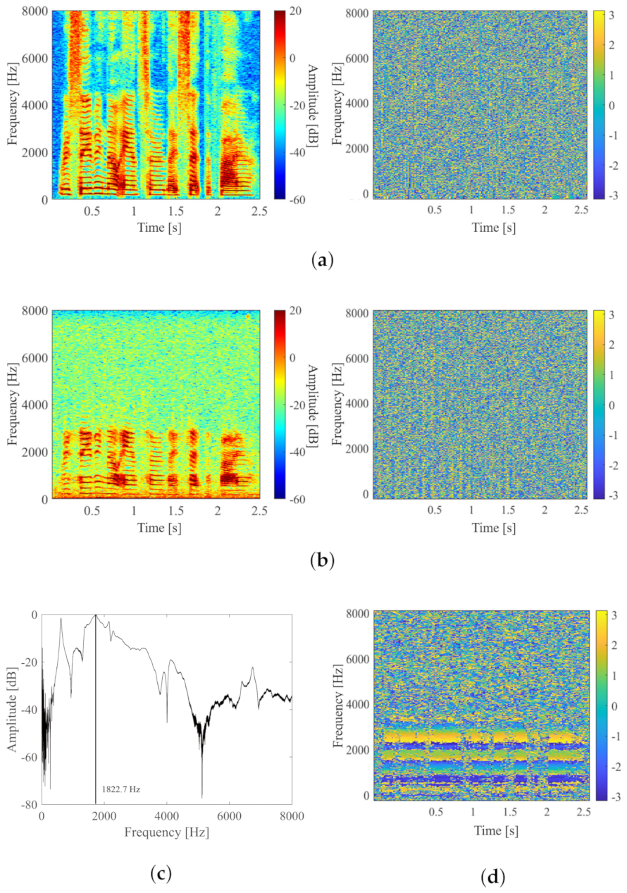
2.1. Problems with Sound Measurement Using LDVs
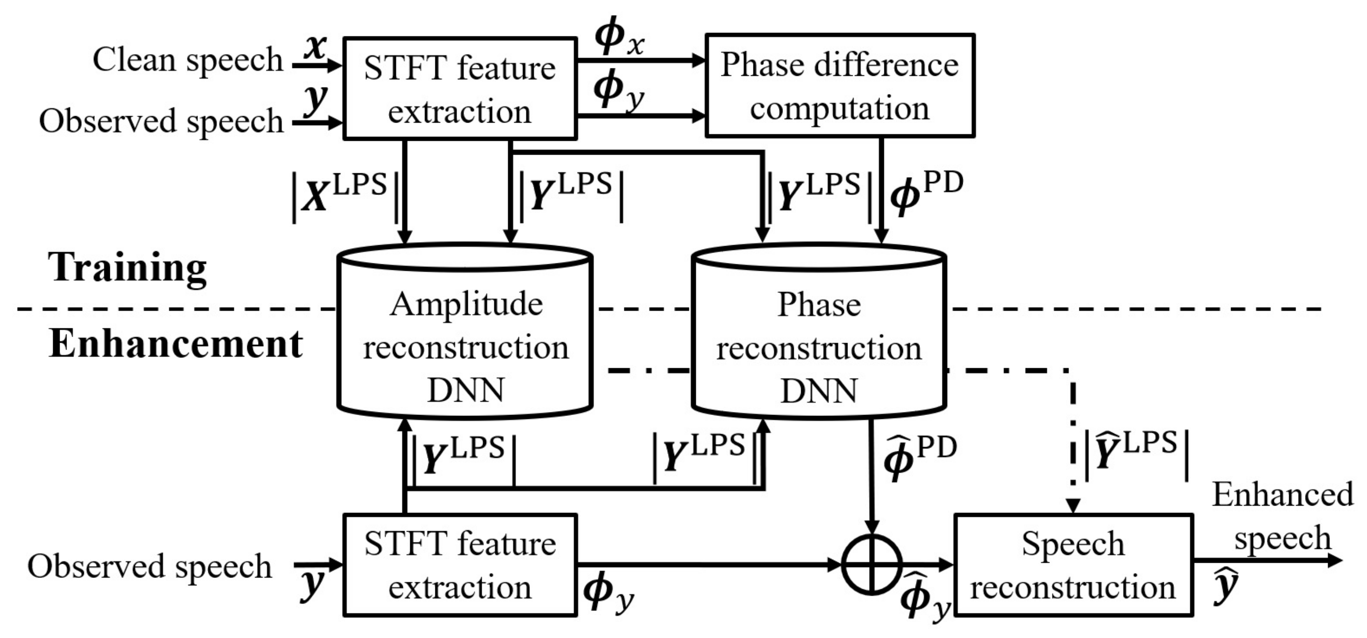
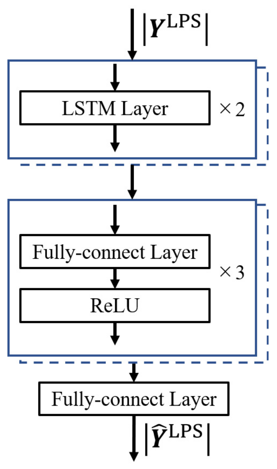
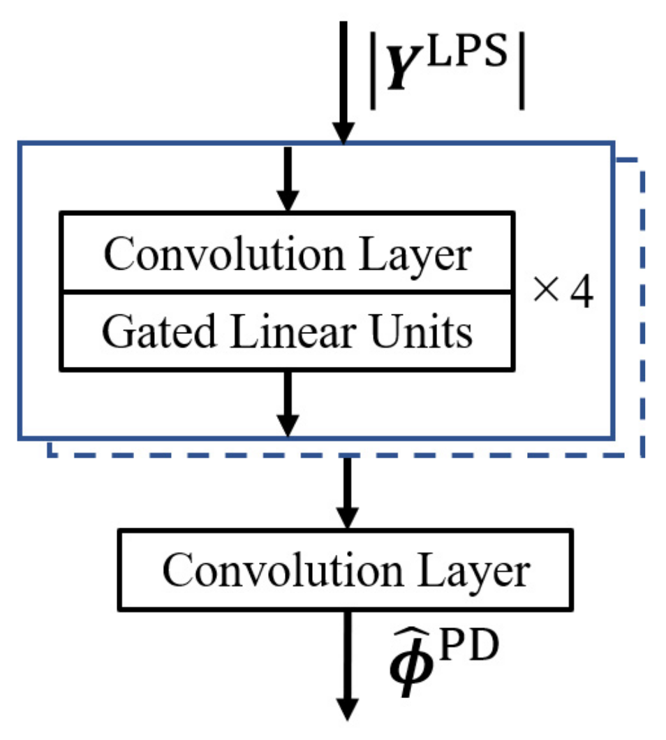
2.2. Stft-Based Speech Enhancement
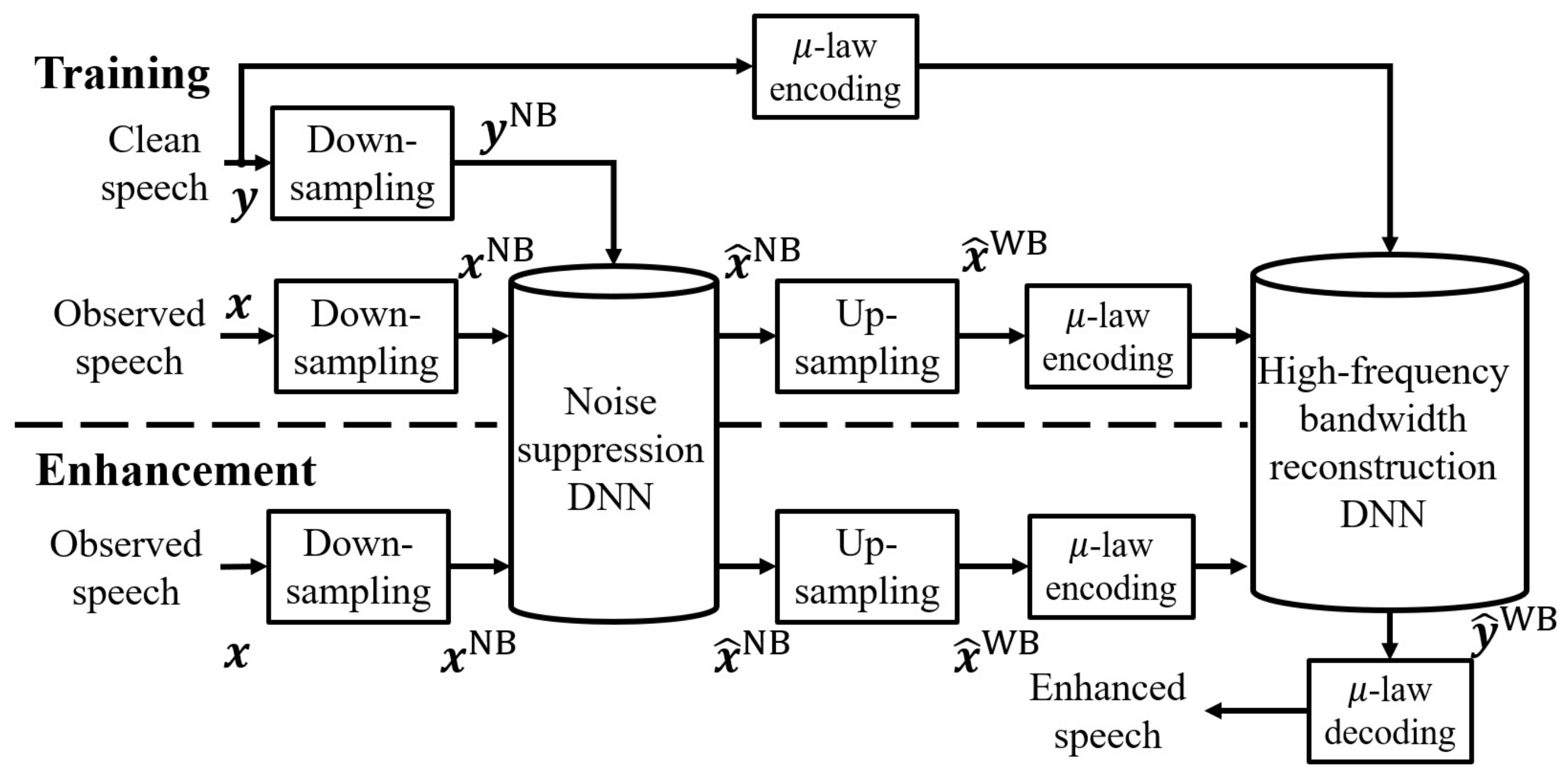
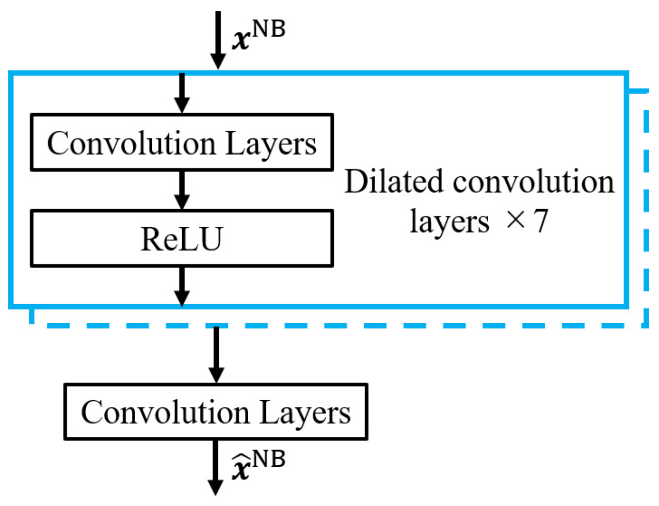
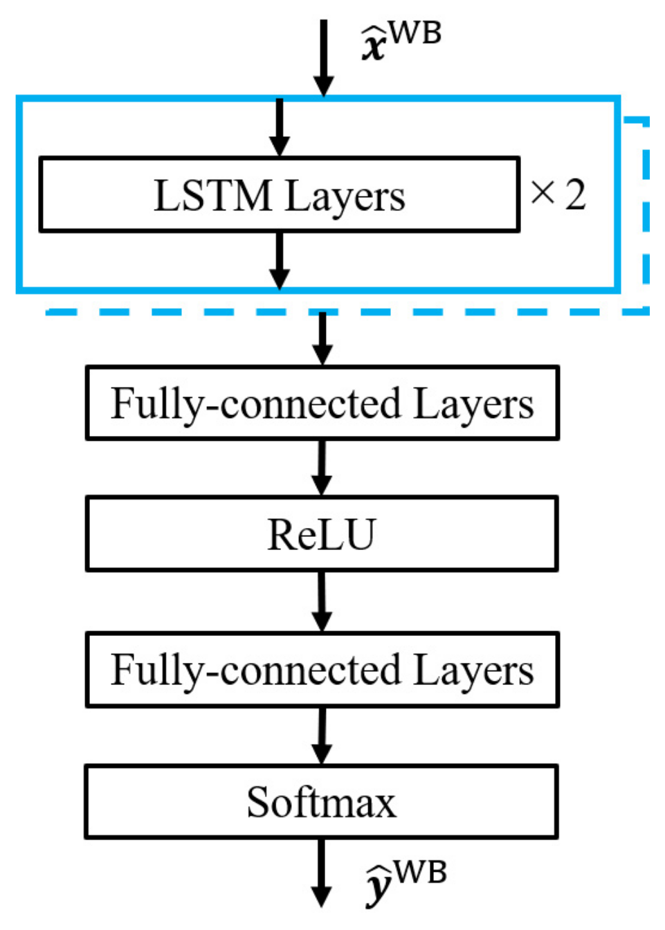
2.3. Waveform-Based Speech Enhancement
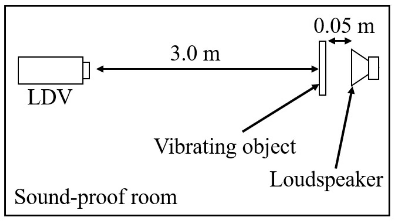
3. Evaluation Experiments
3.1. Training Data Set-Up
3.2. Hyperparameters and Training Conditions
3.2.1. Stft-Based Method
3.2.2. Waveform-Based Method
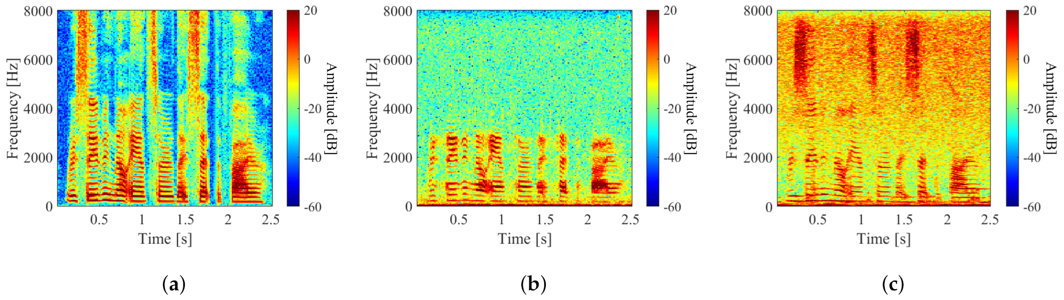
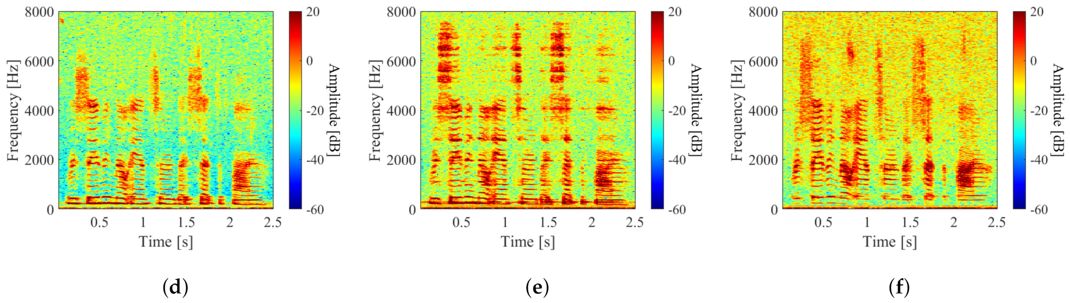
3.3. Evaluation Experiments for Stft-Based Method
3.4. Evaluation Experiment for Waveform-Based Method
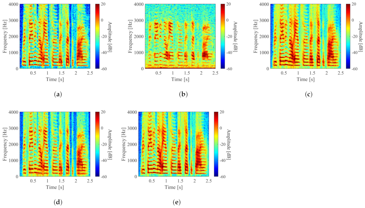
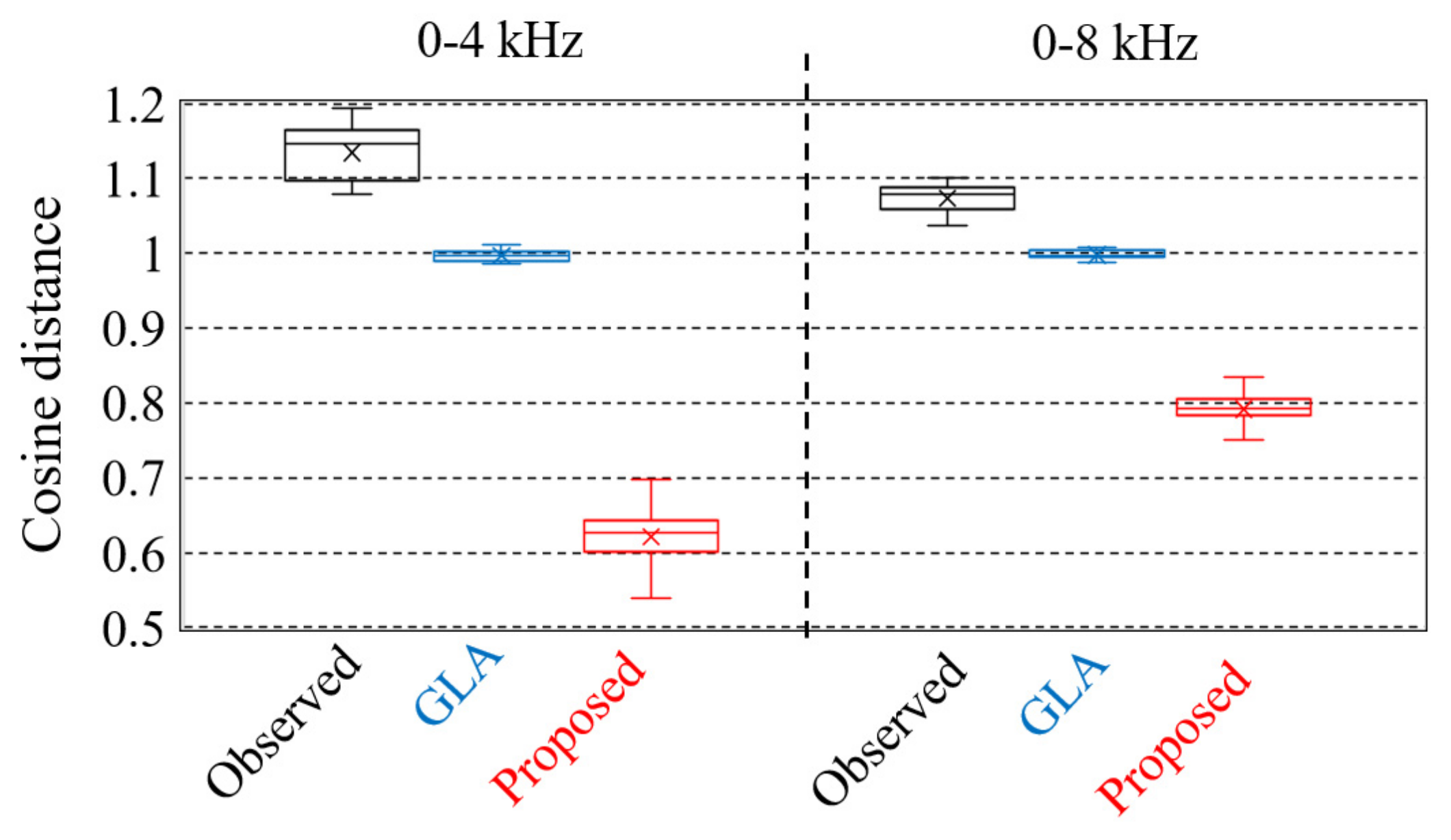
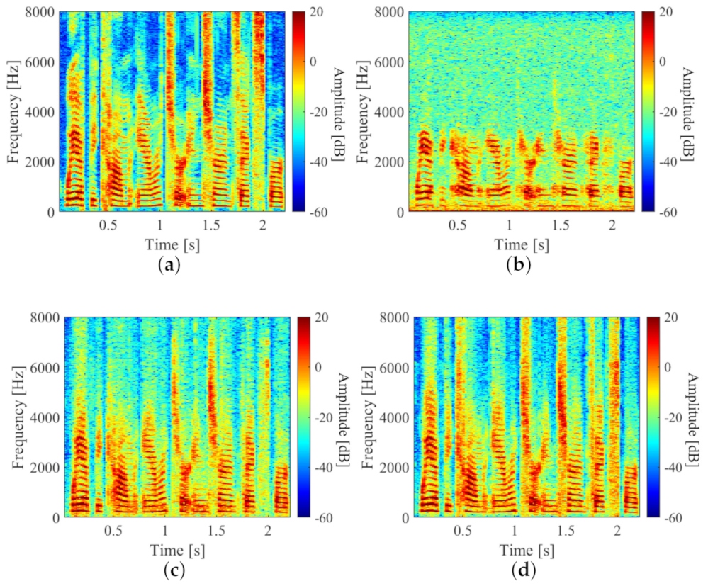
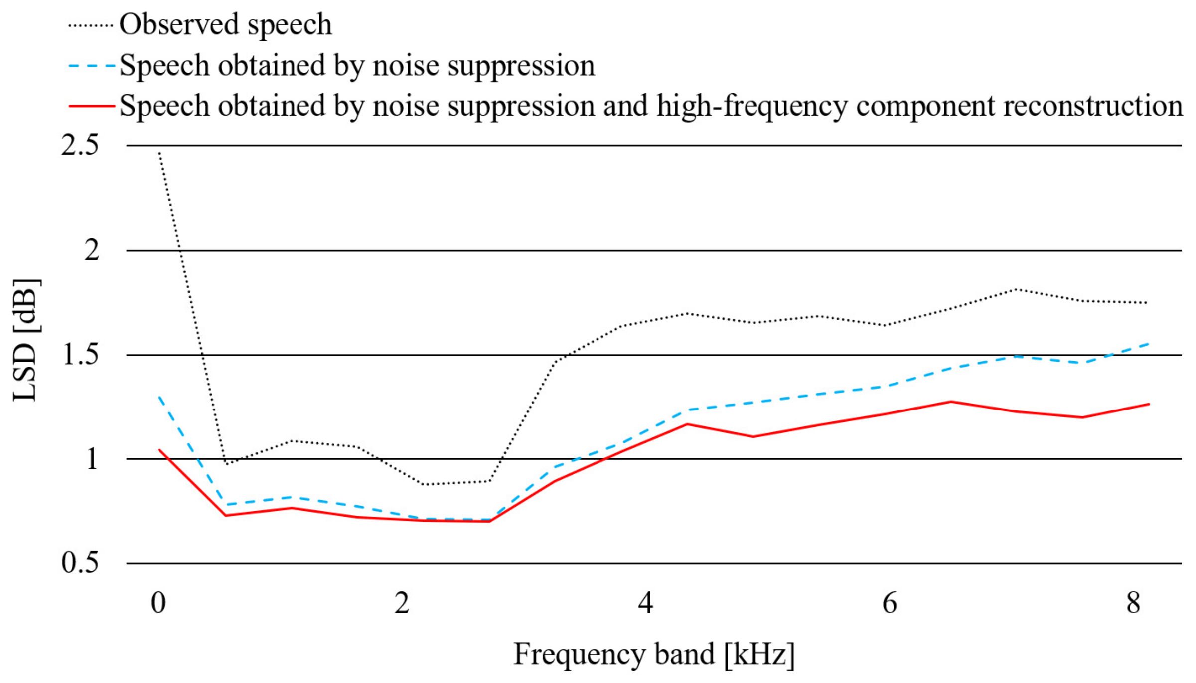
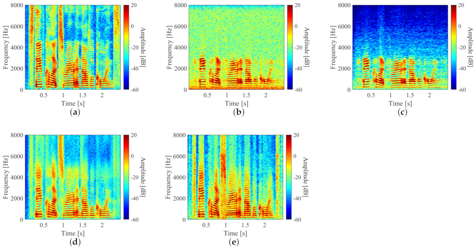
3.5. Evaluation Results and Discussion
4. Conclusions
Author Contributions
Funding
Institutional Review Board Statement
Informed Consent Statement
Data Availability Statement
Conflicts of Interest
References
- Clark, M.A. An acoustic lens as a directional microphone. Trans. IRE Prof. Group Audio 1953, 25, 1152–1153. [Google Scholar]
- Taylor, K.J. Absolute measurement of acoustic particle velocity. J. Acoust. Soc. Am. 1976, 59, 691–694. [Google Scholar] [CrossRef]
- Shang, J.H.; He, Y.; Liu, D.; Zang, H.G.; Chen, W.B. Laser Doppler vibrometer for real-time speech-signal acquirement. Chin. Opt. Lett. 2009, 7, 732–733. [Google Scholar] [CrossRef]
- Leclère, Q.; Laulagnet, B. Nearfield acoustic holography using a laser vibrometer and a light membrane. J. Acoust. Soc. Am. 2009, 126, 1245–1249. [Google Scholar] [CrossRef] [PubMed]
- Avargel, Y.; Cohen, I. Speech measurements using a laser Doppler vibrometer sensor: Application to speech enhancement. In Proceedings of the 2011 Joint Workshop on Hands-free Speech Communication and Microphone Arrays, Edinburgh, UK, 30 May 2011; pp. 109–114. [Google Scholar] [CrossRef]
- Malekjafarian, A.; Martinez, D.; Brien, E.J.O. The feasibility of using laser Doppler vibrometer measurements from a passing vehicle for bridge damage detection. Shock Vib. 2018, 2018, 1–10. [Google Scholar] [CrossRef]
- Chen, D.M.; Xu, Y.F.; Zhu, W.D. Identification of damage in plates using full-field measurement with a continuously scanning laser Doppler vibrometer system. J. Sound Vib. 2018, 422, 542–567. [Google Scholar] [CrossRef]
- Aygün, H.; Apolskis, A. The quality and reliability of the mechanical stethoscopes and Laser Doppler Vibrometer (LDV) to record tracheal sounds. Appl. Acoust. 2020, 161, 1–9. [Google Scholar] [CrossRef]
- Li, W.H.; Liu, M.; Zhu, Z.G.; Huang, T.S. LDV remote voice acquisition and enhancement. In Proceedings of the 18th International Conference on Pattern Recognition, Hong Kong, China, 20–24 August 2006; pp. 262–265. [Google Scholar]
- Peng, R.H.; Xu, B.B.; Li, G.T.; Zheng, C.S.; Li, X.D. Long-range speech acquirement and enhancement with dual-point laser Doppler vibrometers. In Proceedings of the IEEE 23rd International Conference on Digital Signal Processing, Shanghai, China, 19–21 November 2018; pp. 1–5. [Google Scholar]
- Xie, Z.; Du, J.; McLoughlin, I.; Xu, Y.; Ma, F.; Wang, H. Deep neural network for robust speech recognition with auxiliary features from laser-Doppler vibrometer sensor. In Proceedings of the 10th International Symposium on Chinese Spoken Language Processing (ISCSLP), Tianjin, China, 17–20 October 2016; pp. 1–5. [Google Scholar] [CrossRef]
- Lü, T.; Guo, J.; Zhang, H.Y.; Yan, C.H.; Wang, C.J. Acquirement and enhancement of remote speech signals. Optoelectron. Lett. 2017, 13, 275–278. [Google Scholar] [CrossRef]
- Li, K.H.; Lee, C.H. A deep neural network approach to speech bandwidth expansion. In Proceedings of the 2015 IEEE International Conference on Acoustics, Speech and Signal Processing, South Brisbane, QLD, Australia, 19–24 April 2015; pp. 4395–4399. [Google Scholar]
- Lotter, T.; Vary, P. Noise reduction by joint maximum a posteriori spectral amplitude and phase estimation with super-Gaussian speech modelling. In Proceedings of the 12th European Signal Processing Conference, Vienna, Austria, 6–10 September 2004; pp. 1457–1460. [Google Scholar]
- Rethage, D.; Pons, J.; Serra, X. A Wavenet for speech denoising. In Proceedings of the 2018 IEEE International Conference on Acoustics, Speech and Signal Processing, Calgary, AB, Canada, 15–20 April 2018; pp. 5069–5073. [Google Scholar]
- Krawczyk, M.; Gerkmann, T. STFT phase reconstruction in voiced speech for an improved single-channel speech enhancement. IEEE ACM Trans. Audio Speech Lang. Process. 2018, 22, 1931–1940. [Google Scholar] [CrossRef]
- Takamichi, S.; Saito, Y.; Takamune, N.; Kitamura, D.; Saruwatari, H. Phase reconstruction from amplitude spectrograms based on von-mises-distribution deep neural Network. In Proceedings of the 2018 16th International Workshop on Acoustic Signal Enhancement (IWAENC), Tokyo, Japan, 17–20 September 2018; pp. 286–290. [Google Scholar]
- Dauphin, Y.N.; Fan, A.; Auli, M.; Grangier, D. Language modeling with gated convolutional networks. In Proceedings of the 34th International Conference on Machine Learning, Ningbo, China, 6–11 August 2017; pp. 933–941. [Google Scholar]
- Kingma, D.P.; Ba, J. Adam: A method for stochastic optimization. In Proceedings of the 3rd International Conference on Learning Representations, ICLR 2015, San Diego, CA, USA, 7–9 May 2015. [Google Scholar]
- Recommendation, I.G. 711: Pulse code modulation (PCM) of voice frequencies. Int. Telecommun. Union 1988. [Google Scholar]
- Ledig, C.; Theis, L.; Huszar, F.; Caballero, J.; Cunningham, A.; Acosta, A.; Aitken, A.; Tejani, A.; Totz, J.; Wang, Z.; et al. Photo-realistic single image super-resolution using a generative adversarial network. arXiv 2017, arXiv:1609.04802. [Google Scholar]
- He, K.; Zhang, X.Y.; Ren, S.Q.; Sun, J. Delving deep into rectifiers: Surpassing human-level performance on ImageNet classification. In Proceedings of the IEEE International Conference on Computer Vision, Santiago, Chile, 7–13 December 2015; pp. 1024–1034. [Google Scholar]
- Garofolo, J.S.; Lamel, L.F.; Fisher, W.M.; Fiscus, J.G.; Pallett, D.S.; Dahlgren, N.L. Acoustic-Phonetic Continuous Speech Corpus CD-ROM NIST Speech Disc 1-1.1; NASA STI/Recon Tech. Rep. LDC93S1; Linguistic Data Consortium: Philadelphia, PA, USA, 1993; Volume 93. [Google Scholar]
- Werbos, P.J. Backpropagation through time: What it does and how to do it. Proc. IEEE 1990, 78, 1550–1560. [Google Scholar] [CrossRef]
- Griffin, D.; Lim, J. Signal estimation from modified short-time Fourier transform. IEEE Trans. Audio Speech Lang. Process. 1984, 32, 236–243. [Google Scholar] [CrossRef]
- Perraudin, N.; Balazs, P.; Sondergaard, P.L. A fast Griffin-Lim algorithm. In Proceedings of the 2013 IEEE Workshop on Applications of Signal Processing to Audio and Acoustics, New Paltz, NY, USA, 20–23 October 2013; pp. 1–4. [Google Scholar]
- Wang, P.; Wang, Y.; Liu, H.; Sheng, Y.; Wang, X.; Wei, Z. Speech enhancement based on auditory masking properties and log-spectral distance. In Proceedings of the 3rd International Conference on Computer Science and Network Technology, Dalian, China, 12–13 October 2013; pp. 1060–1064. [Google Scholar] [CrossRef]


| Variable | Signification | Variable | Signification |
|---|---|---|---|
| Clean speech | Phase spectrum of clean speech | ||
| Observed speech | Phase spectrum of observed speech | ||
| Narrow-band clean speech | Phase difference between and | ||
| Narrow-band observed speech | K | Fourier transform length | |
| Wide-band clean speech | k | Frequency index | |
| Wide-band observed speech | m | Frame index | |
| | | Log-power spectrum of clean speech | n | Sampling index |
| | | Log-power spectrum of observed speech | Estimated value |
| Environment | Sound-Proof Room |
|---|---|
| Ambient noise level | 20.8 dB |
| Sampling frequency | 16 kHz |
| Sound pressure of sound source | 85 dB(A) |
| Quantization bit rate | 16 bits |
| Data | TIMIT Acoustic Phonetic |
| Continuous Speech Corpus | |
| 9000 files (8 h) for training | |
| 240 files (12 min) for validation | |
| Audio interface | Roland OCTA-CAPTURE UA-1010 |
| LDV Equipment type | Polytec VibroFlex Xtra VFX-I-120 |
| Software & libraries | Matlab R2022a, Deep learning HDL tool box v1.3 |
| Vibrating object | PET-bottle |
| PESQ Score | LSD [dB] | STOI Score | |
|---|---|---|---|
| (b) | 1.76 ± 0.40 | 1.62 ± 0.10 | 0.85 ± 0.04 |
| (c) | 2.25 ± 0.35 | 2.17 ± 0.30 | 0.87 ± 0.04 |
| (d) | 2.25 ± 0.30 | 1.09 ± 0.08 | 0.93 ± 0.02 |
| (e) | 2.35 ± 0.30 | 1.11 ± 0.08 | 0.94 ± 0.03 |
Disclaimer/Publisher’s Note: The statements, opinions and data contained in all publications are solely those of the individual author(s) and contributor(s) and not of MDPI and/or the editor(s). MDPI and/or the editor(s) disclaim responsibility for any injury to people or property resulting from any ideas, methods, instructions or products referred to in the content. |
© 2023 by the authors. Licensee MDPI, Basel, Switzerland. This article is an open access article distributed under the terms and conditions of the Creative Commons Attribution (CC BY) license (https://creativecommons.org/licenses/by/4.0/).
Share and Cite
Cai, C.; Iwai, K.; Nishiura, T. Speech Enhancement Based on Two-Stage Processing with Deep Neural Network for Laser Doppler Vibrometer. Appl. Sci. 2023, 13, 1958. https://doi.org/10.3390/app13031958
Cai C, Iwai K, Nishiura T. Speech Enhancement Based on Two-Stage Processing with Deep Neural Network for Laser Doppler Vibrometer. Applied Sciences. 2023; 13(3):1958. https://doi.org/10.3390/app13031958
Chicago/Turabian StyleCai, Chengkai, Kenta Iwai, and Takanobu Nishiura. 2023. "Speech Enhancement Based on Two-Stage Processing with Deep Neural Network for Laser Doppler Vibrometer" Applied Sciences 13, no. 3: 1958. https://doi.org/10.3390/app13031958