Article

Performance Assessment of the Medium Frequency R-Mode Baltic Testbed at Sea near Rostock

by
Filippo Giacomo Rizzi
1,*,†,
Lars Grundhöfer
1,†,
Stefan Gewies
1,† and
Tobias Ehlers
2,†
1
Institute of Communications and Navigation, Nautical Systems Department, German Aerospace Center (DLR), Kalkhorstweg 53, 17235 Neustrelitz, Germany
2
German Federal Maritime and Hydrographic Agency (BSH), Bernhard-Nocht-Straße 78, 20359 Hamburg, Germany
*
Author to whom correspondence should be addressed.
These authors contributed equally to this work.
Appl. Sci. 2023, 13(3), 1872; https://doi.org/10.3390/app13031872
Submission received: 21 December 2022 / Revised: 24 January 2023 / Accepted: 29 January 2023 / Published: 31 January 2023
(This article belongs to the Special Issue Applied Maritime Engineering and Transportation Problems 2022)

Abstract

:
Global Navigation Satellite Systems (GNSS) are the primary source of position, navigation and timing (PNT) information in the maritime domain. Nevertheless, there is a pressing need for alternative absolute position information to serve as a backup when GNSS is not trustworthy or usable. One possible alternative navigation system is the terrestrial Ranging Mode, also known as the R-Mode. It reuses medium frequency (MF) radio beacons and base stations of the very high frequency data exchange system (VDES) for the transmission of synchronised signals in the service areas of those stations. A large-scale R-Mode testbed is available in the southern Baltic Sea with eight MF radio beacons transmitting R-Mode signals. These signals suffer the self-interference generated by the reflection of the radio wave from the ionosphere at night. The reflected signal, known as the sky wave in the literature, is a form of multipath, which decreases the accuracy of the system. In our work, we present the analysis of measurements obtained with the research vessel Deneb. The horizontal accuracy achieved in the optimal condition was 15.1 m (95%), whereas under the sky wave, the accuracy decreased to 55.3 m. The results are a starting point for the further development of the MF R-Mode system.

1. Introduction

Today, position, navigation and timing (PNT) services play a fundamental role in different areas of our society. Their use is widespread, from the provision of information to mass-market devices, such as smartphones and wearables, to safety–liability critical devices, where a trustworthy position or time data becomes vital [1]. Global Navigation Satellite Systems (GNSS) are the primary sources of such information, given their global coverage and high reliability, and particularly for the maritime sector, where the nominal functionality of multiple devices on board ships and vessels entirely depends on such systems. Clearly, this can be a single point of failure, endangering crew members and passengers, goods and the environment.
In recent years, an increase in the number of threats to GNSS receivers has been observed, rising the concerns of the research community in the field of navigation [2,3]. Different research approaches have been considered in order to address this problem, such as jamming and spoofing detection and countermeasures [4], improvements of the transmitted GNSS signals with authentication services such as the Galileo Open Service Navigation Message Authentication (OSNMA) [5], or integration with additional sensors (e.g., inertial measurement unit, inertial navigation system, Camera, Lidar, and Radar). A further promising approach is the establishment of A(lternative)PNT systems, which replace GNSS in the case of outages or interference events.
The Ranging Mode (R-Mode) is a terrestrial navigation system based on the signals of the opportunity approach, which is currently under development in the Baltic Sea [6], where a testbed is now operational. The key idea of the R-Mode is to reuse the existing infrastructure to diminish the cost of implementation and deployment. Maritime radio beacons transmitting in the 300 kHz medium frequency (MF) band and the Automatic Identification System (AIS), or its modernised version, known as the very high frequency data exchange system (VDES), working at frequencies around 162 MHz, are used, in particular [7,8]. Initial studies on the R-Mode have been conducted by several authors assessing the feasibility of the system [9,10,11].
This paper presents the results of a measurements campaign conducted in the Baltic Sea near Rostock. At the time of the campaign, only maritime radio beacons, referred to as MF stations throughout the paper, were available in the testbed. Therefore, only the performance of the MF R-Mode system will be demonstrated.
MF signals are affected by different impairments, which will be briefly described in the paper. Among them, the sky-wave effect, a multipath reflection, which appears mainly at night when the solar radiation is low, is of primary concern. The self-interference generated by the sky-wave can degrade the system accuracy, and predicting such an effect is quite complex, since it depends on solar radiation effects such as day–night variation [12], seasonal variation, solar cycles and distance between receiver and transmitter, just to mention a few [13]. The initial performance results have already been presented in [14], demonstrating that it is possible to achieve a positioning accuracy of 12 m (95%), but only during the day. In this work, the night-time results are also presented and discussed.
The paper is organized as follows: Section 2 describes the MF R-Mode system in a nutshell, with some of the relevant information on the testbed and receiver specification. In Section 3, the impairments of the R-Mode MF signals are presented, with a particular focus on the description of the sky-wave multipath effect. Section 4 contains the results of the measurement campaign during the daytime and nighttime. Finally, Section 5 concludes the paper.

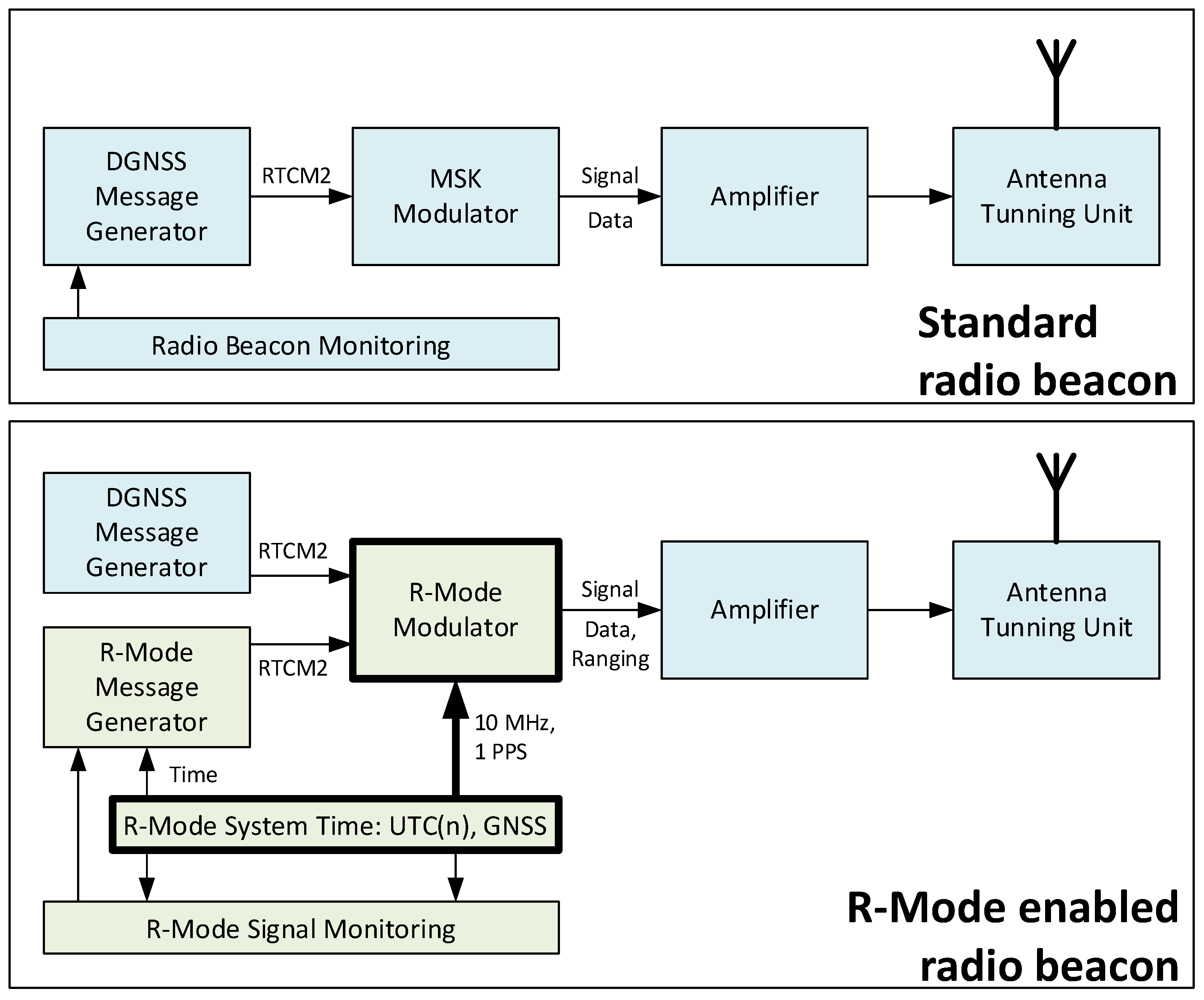
2. The MF R-Mode System

One of the main outcomes of the R-Mode Baltic project was the successful establishment of a testbed in the Baltic Sea. At the time of writing, the testbed includes eight operational MF radio beacons transmitting R-Mode signals. Figure 1 shows the map of the testbed area with the position of the R-Mode-enabled radio beacons located in four countries: Germany, Sweden, Poland and Denmark.
The MF radio beacon system is based on the Frequency Division Multiple Access (FDMA) scheme. Thus, a channel of 500 Hz is allocated for each terrestrial beacon in the marine frequency band between 283.5 kHz and 315 kHz. These values are valid in European countries and might differ in other regions, where a different frequency allocation strategy has been selected. An important characteristic of the radio waves in the MF band is that they propagate as a ground-wave. This means that the signals are not limited to the line-of-sight (LOS) propagation, as it is for GNSS or VHF signals, but they propagate far beyond the horizon following the curvature of the earth. Therefore, the R-Mode positioning only provides 2D solutions and does not provide any height information. The transmitted signal includes a Minimum Shift Keying (MSK)-modulated signal, which represents the legacy signal carrying the D(ifferential) GNSS information, plus two additional pilot signals, each referred to as a Continuous Wave (CW). Such sinusoidal signals are placed in the fourth zero crossing of the MSK spectrum to minimize interference on the legacy signal and, to be precise, they are spaced by 225 Hz on the left and right of the carrier frequency. Additionally, the signals are synchronized to the R-Mode System Time in order to have a zero-phase crossing to the full seconds, such that synchronization is achieved among all the transmitters. The R-Mode System Time is the reference time for all R-Mode system components. It can be aligned to the GPS time, as it is conducted by the GPS-stabilized rubidium clocks at the moment but also other options are possible, such as the time and frequency transfer using fiber optic cable. The research on cost-efficient synchronization strategies is ongoing [15].
The fundamental idea to obtain pseudorange measurements at the receiver side is to exploit phase estimates of the two CW and to track the evolution of these phases as the vessel moves. This technique is similar to the one used in the GNSS receivers, which exploit carrier phase observations to obtain high-accuracy positioning solutions [16]. The pseudorange ρ j , k ( t ) can then be represented as follows
ρ j , k ( t ) = [ N j , k ( t ) + ϕ j , k ( t ) + ϕ j , k c k + ϕ j , k ϵ ] λ j , k
where j is the station index and k = 1 , 2 is an index which distinguishes between the two CW. λ is the wavelength of the CW. N represents the integer number of the full wavelengths between the transmitter and the receiver, referred to as the ambiguity in the GNSS domain, and ϕ j , k represents the fractional part of the wavelength. Finally, ϕ j , k c k represents the error caused by the clock at the receiver and transmitter side j, while ϕ j , k ϵ includes the errors introduced by the different impairments encountered by the signal, as will be explained in Section 3.
A Software-Defined Radio (SDR) receiver has been developed by the DLR, as described in [14]. The receiver setup is composed of an Ettus X310 connected to an E-field antenna through an amplifier and a filter. These components represent the front-end of the receiver, which provides as an output the discretized digital raw samples to a computer. A C++ and Python-based receiver implementation performs digital signal processing and phase and position estimation on the computer. As explained, the phase measurements are characterized by the presence of the ambiguity, which needs to be estimated. Due to the fact that the transmitters and receiver are not calibrated, the current implementation of the receiver solves the ambiguity by using a calibration process. The mechanism is based on the knowledge of the accurate location provided by the GNSS receiver at the time of calibration. A 30 s averaging time window allows one to calibrate the measurements and solve the ambiguities for all the available signals [14]. Afterwards, the tracking is in charge of computing the accumulated phase measurements. With the calibrated measurements, the receiver can estimate the latitude and longitude in the WGS-84 coordinate frame and the receiver time offset by using an iterative least squares algorithm. Due to the signal propagation, the transmitter–receiver distance is modelled by the Vincenty’s formula [17], which gives the distance between two points on the WGS-84 ellipsoid, assuming that the height of the two points is zero. Further details on the least squares algorithm are given in [14].

3. Mf Signal Impairments

The propagation of MF signals is characterized by a variety of impairments which need to be considered when these signals are used for positioning purposes. From this point of view, the main two challenges in obtaining an accurate positioning performance in the MF R-Mode system are the following: mitigating the sky-wave reflection arriving from the ionosphere at night, and predicting the wave-propagation delay induced by the variation of the electrical properties of the atmosphere and ground along the propagation path. In the following sections, the two issues will be briefly described. Furthermore, a third issue concerning the possible transmitter instability is also discussed.

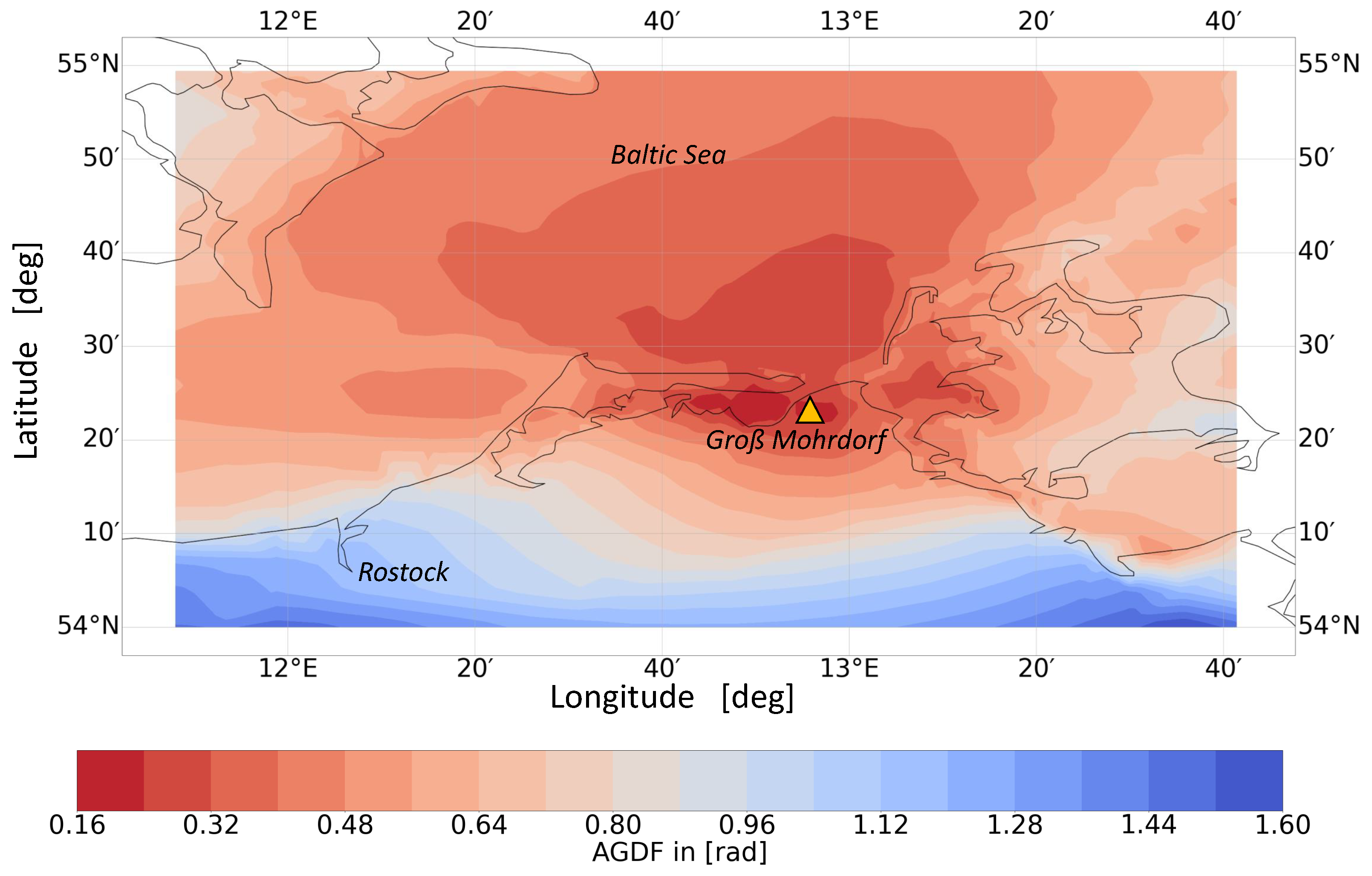
3.1. Atmospheric and Ground Delay Factor (AGDF)

MF signals propagate along the earth’s surface as the ground-wave [18]. This is an essential characteristic, which allows the signal to travel over longer distances in comparison to the line-of-sight propagation limitation, which is typical for higher frequency signals. Above the ground, the atmospheric refractive index causes a propagation speed reduction which becomes visible as a delay of the signal in the time domain. Furthermore, at the earth’s surface, the signal encounters different types of land and water segments which are characterized by different materials with specific electrical properties. Each of these segments has a specific ground conductivity and electric permittivity, which produce a damping of the signal’s amplitude and a further change of propagation speed [19]. The overall delay experienced by the signal has been defined as AGDF [20].
It is possible to predict the AGDF for an arbitrary propagation path composed by several sections of different electrical properties by using the ITU World Atlas of Ground Conductivities [21]. For each section, the attenuation and delay of the signal is computed with the method introduced by Rotheram [22,23] and Wait [24]. Finally, the overall delay is obtained through the application of the Millington/Pressey method, as explained in [24,25].
As an example, Figure 2 shows the phase delay in radians with respect to the propagation in the vacuum for the signal transmitted by the radio beacon located in Groß Mohrdorf, Germany, over the southern Baltic Sea. It is caused by the refractive index of the atmosphere, here assumed to be constant, and the variation of the ground conductivity, as given in the ITU maps.
Measurements in specific areas can be used to apply an enhanced correction technique on these AGDF maps to improve the R-Mode performance [20].

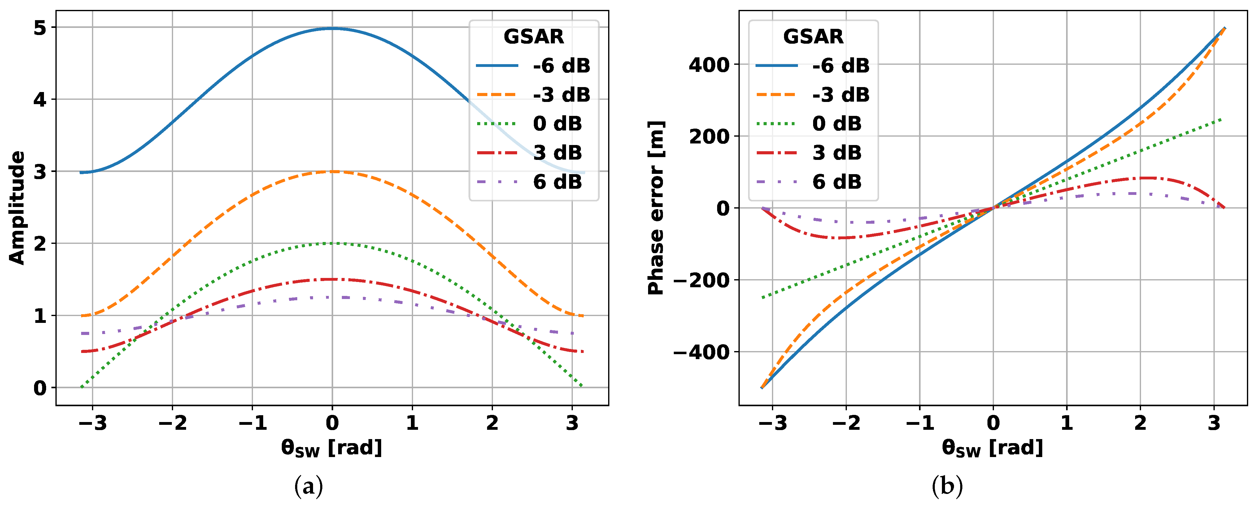
3.2. Sky-Wave Self-Interference

MF radio waves can travel either as ground-waves, by following the earth’s surface, or as a sky-wave reflection between the earth and the ionosphere [18]. While the ground-wave is characterized by the propagation phenomena, which attenuate and delay the signal, as described in Section 3.1, the sky-wave can be observed as a multipath effect which generates self-interference on the receiver side, degrading the ranging accuracy. This effect depends on several factors, such as the frequency of the signal itself, the ionospheric reflection height, the angle of the incidence, the geographical region of interest and solar activity [13].
Radio waves in the 300 kHz frequency range are significantly absorbed by the D-layer of the ionosphere during the daytime. Therefore, the sky-wave interference effect is negligible, since its field strength is far smaller than the ground-wave in the service area of the radio beacon. In contrast, at night, the D-layer tends to disappear. The signal is therefore no longer attenuated and hits the upper ionospheric E-layer, which is capable of reflecting signals below 10 MHz.
In a simplified scenario, we can assume a one-ray reflection model, where the sky-wave sum-up to the ground-wave signal at the receiver side. By neglecting the influence of the noise, we can define the real value ground-wave signal, as follows
s GW = A GW ( t ) cos ( 2 π f t + θ GW )
where A GW is the signal amplitude, f is the frequency of a particular CW and θ GW is the phase shift due to the propagation path. Similarly, the sky-wave can be given as follows
s SW = A SW ( t ) cos ( 2 π f t + θ SW )
where now A SW represents the sky-wave amplitude, and θ SW is the phase shift due to the sky-wave propagation path, which clearly differs from the ground-wave one. The sum of the two signals can be expressed as follows
s SUM = s GW + s SW = A SUM ( t ) cos ( 2 π f t + θ SUM )
where
A SUM = A GW 2 + A SW 2 + 2 A GW A SW cos ( θ GW θ SW )
and
tan ( θ SUM ) = A GW sin ( θ GW ) + A SW sin ( θ SW ) A GW cos ( θ GW ) + A SW cos ( θ SW ) .
The derivation of Equations (4)–(6) is given in the Appendix A.
We attempt to explain the impact of a sky-wave on the phase error and amplitude in a simulated scenario. We assume A GW = 1 , θ GW = 0 for simplicity and we define the ground-wave to the sky-wave amplitude ratio (GSAR) as follows
GSAR = A GW A SW .
With these assumptions, Equation (6) becomes
θ SUM = tan 1 sin ( θ SW ) GSAR + cos ( θ SW ) = θ e r r
and θ SUM directly represents the phase error θ e r r .
We now demonstrate the amplitude and phase error obtained under the influence of sky-wave interference for different GSAR and θ GW . Figure 3 presents the amplitude of the sum signal on the left (Figure 3a) and the phase error with respect to the ground wave on the right side (Figure 3b) for ground-wave-dominated (GSAR = 6 dB) to sky-wave-dominated (GSAR = −6 dB) conditions. Starting from the amplitude plot, we can observe that, as the GSAR decreases, the amplitude estimate can be greater or smaller than the true one. In particular, this depends on the phase difference between the ground-wave and the sky-wave and on the GSAR, which influences the resulting interference. When the phase difference is zero, the interference is constructive, which means that the signal strength, or amplitude, increases, and the reach is the maximum. In contrast, when the signals are out of the phase ( π or π ), the interference is destructive and the signal strength decreases.
Nevertheless, for positioning purposes, the estimated phase or phase error respective to the true value is more important than the amplitude itself. By looking at the phase error represented in Figure 3b, we can observe that with the decrease in GSAR, the phase error increases, in the absolute value sense. If GSAR ≤ 1, the error always increases monotonically with the increase in the sky-wave phase. The maximum absolute value error is π or half the wavelength. In such a case, the sky-wave is stronger than the ground-wave, which means that the receiver will finally track the sky-wave, severely corrupting the range estimation. This is clearly the worst possible situation. For GSAR > 1, we can observe that the phase error has a maximum, in the absolute value sense, between 0 and π . This maximum depends on the value of the GSAR and is given by the following formula
θ err = tan 1 1 GSAR 2 1 .
The reader can find the derivation of Equation (9) in the Appendix A.
The mitigation of the sky-wave interference poses a real challenge to the usage of the MF R-Mode system, and research in this field is ongoing. One of the possible solutions would be to redesign the signal waveform modulation in order to have a broader signal bandwidth, which would allow the receiver to distinguish between the ground-wave and the reflected wave at the receiver side, as suggested in [26]. An alternative approach is to design specific antenna patterns in order to attenuate signals arriving with high elevation angles, which most likely are sky-waves [18]. The transmitter antenna pattern is generally optimized to transmit the signals horizontally. Therefore, the sky-wave is negligible in the vicinity of the transmitter, due to the transmitter antenna pattern, even if the receiver antenna is assumed to be isotropic. The sky-wave becomes stronger at larger distances where the reflected wave, generated by the transmitter antenna, presents a dependency on the elevation angle. Thus, having a non-isotropic receiving antenna with a specific pattern could help in mitigating the influence of the sky-wave.

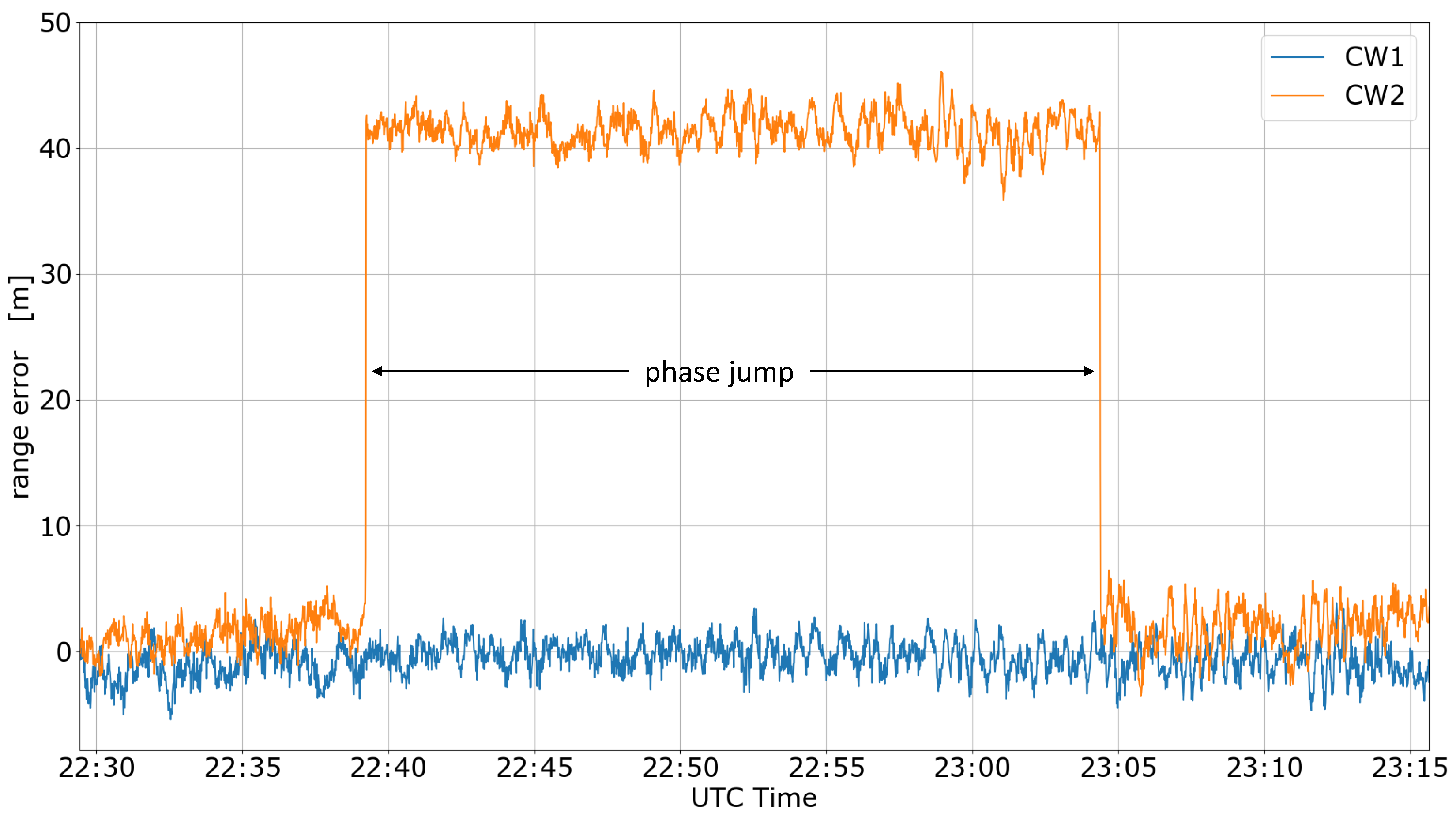
3.3. Transmitter Instability

MF radio beacons were not initially designed to be used as a stand-alone positioning system. Therefore, some adaptations and modifications are needed for the hardware on the transmitter side. In principle, these adjustments, needed to enable R-Mode signals transmission, could be easily implemented at the sites. Figure 4 presents the generalized difference in architecture between a standard DGNSS beacon and an R-Mode-enabled radio beacon. First of all, the MSK modulator must be replaced with an R-Mode modulator, then, two additional components are required: an R-Mode message generator and a stable and accurate timing source synchronized with the R-Mode system time. The last component required is an R-Mode signal monitor. This solution is extremely cost-efficient when compared to the deployment of a new GNSS satellite.
Nevertheless, the hardware components in the standard radio beacons are not identical. They differ depending on the country. In general, different manufacturer and different hardware specifications might be used in different countries. For this reason, transmitter-side instability effects can be observed for some radio beacons but not for others, even in the same country. As an example, we show in Figure 5 an issue that was identified at the Groß Mohrdorf station. In detail, a phase jump in the order of 40 m is visible for Groß Mohrdorf, lasting approximately 25 min. It is interesting to observe that the jump affects one of the signals, the CW2, but not the other. This behaviour was observed from time to time, with varying severity—a clear cause has not yet been identified. In the future, these instabilities can be avoided by identifying their source or by using monitor stations with correction information sent to the R-Mode users by specific R-Mode messages.
Part of the analysis and characterization of the transmitter chain has already started, as presented in [27]. In future projects, a deeper and more accurate analysis of the transmitter chain will be carried out in order to identify the source of such instabilities and implement a solution. Alternatively, on the receiver side, a detection mechanism in combination with a correction or exclusion technique can be applied to solve this issue.

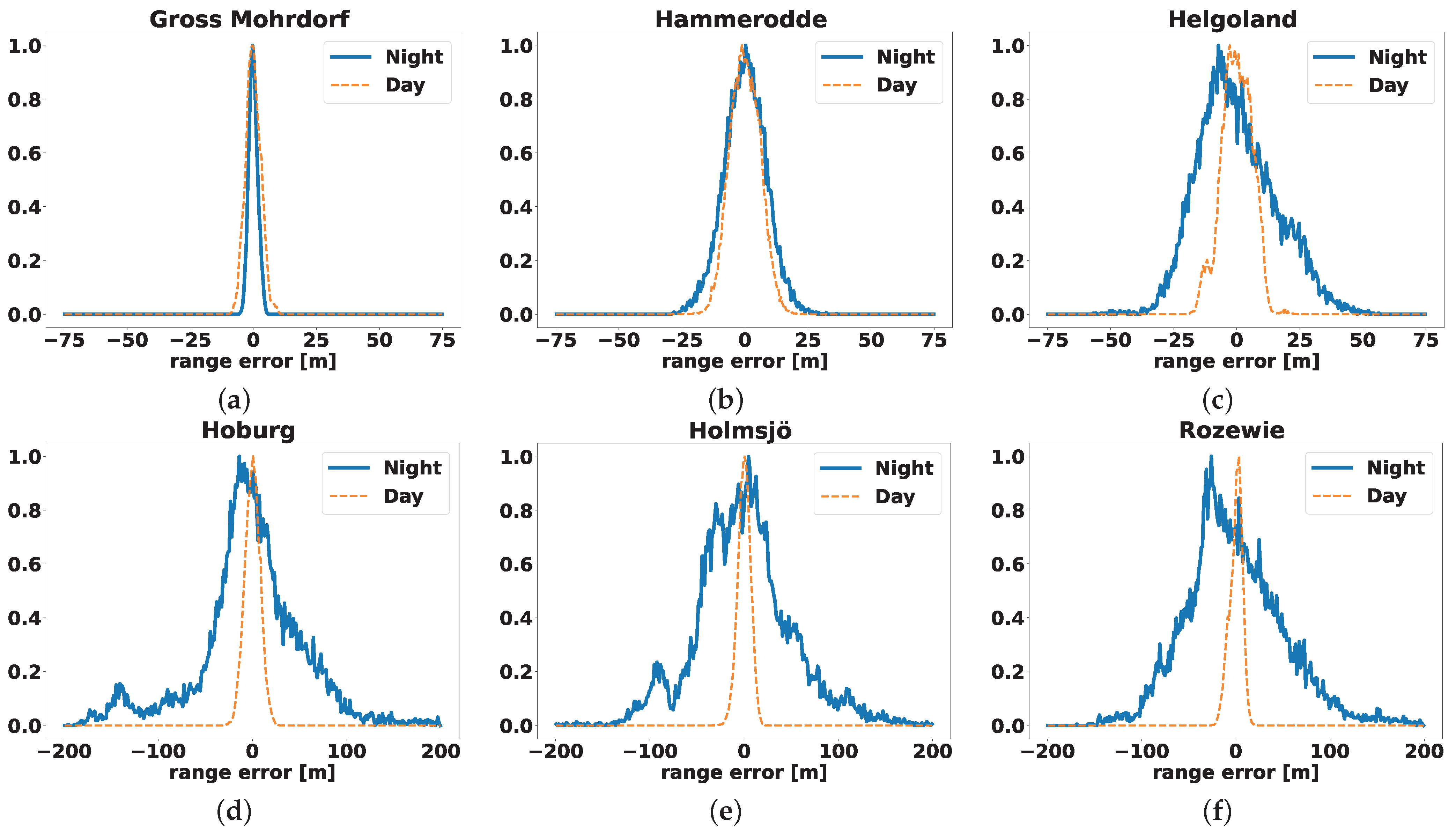
4. Mf R-Mode System Accuracy: Results and Discussion

In this section, the performance of the system will be demonstrated mainly in terms of the horizontal positioning accuracy for the daytime scenario, with a negligible impact of the AGDF, and for the nighttime one with the presence of sky-waves. In February 2021, the DLR, with the support of the partners involved in the R-Mode Baltic project, performed a measurement campaign in the southern Baltic Sea on board the vessel Deneb that was provided by the BSH. The test area is located near Rostock and is visible in Figure 6 as a red rectangle. During the measurement campaign, only six out of the eight available R-Mode transmitters were operational, namely Groß Mohrdorf, Rozewie, Hammerodde, Helgoland, Holmsjö and Hoburg. They are visible as yellow triangles in Figure 6.
An interesting piece of information to keep in mind is the distance between the different MF radio beacons and the centre of the test area. This is given in Table 1. As is clear, some of the stations were located at a distance greater than the assumed approximated coverage of 250 km, such as Hoburg, Rozewie and Holmsjö. Despite the significant distance, they were received with good accuracy during the day, as will be demonstrated in the next section, while they were excluded from the positioning solution at night due to the strong influence of the sky-waves.
The DLR receiver was operating with a sampling frequency of 1 MHz, and the observation time for the Fast Fourier Transform (FFT) algorithm, which provides phase estimates, was set to 1 s. Measurements with 1 Hz frequency resolution were therefore obtained. A GPS-stabilized rubidium clock, which ensured the synchronization with GPS time, was used in the setup. This is in general not required, but it is relevant in a research and development phase to assure stable measurements, helping in the identification of further problems or issues. Additionally, the setup included a Saab R5 GNSS receiver operating in a real-time kinematic (RTK) mode by using the Hemisphere Atlas Global Correction Service, which assured a very accurate reference track, with an accuray of 8 cm (95%) [28], and was used to determine the R-Mode horizontal positioning error.

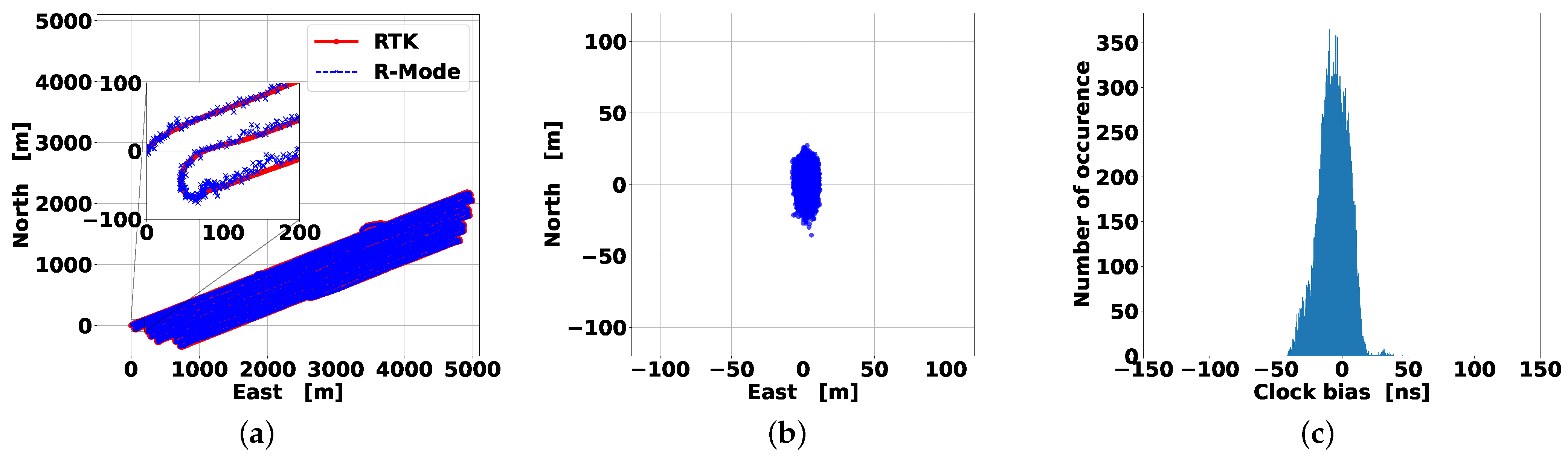
4.1. Daytime Results

The results presented in this section are related to data recorded during the day. Moreover, the impact of the AGDF for this data set was almost negligible, due to the limited area in which the vessel was operating. We therefore rate the scenario as “optimal” in the sense that the achievable accuracy depends mainly on the receiver noise and the signals’ received power. The data set was recorded between 7:56 UTC and 14:00 UTC, and at least one signal per radio beacon was usable during this time. This means that all the transmitters were used in the positioning solution. The signals used are visible in Table 2 with the “h” flag, which stands for healthy, whereas the unusable signals are indicated as unhealthy with the “uh” flag. The unhealthy flag was set for some of the signals due to the observed transmitter instabilities, as explained in Section 3.3.
Figure 7a presents the R-Mode positioning solution, as blue crosses, in a local reference frame (east-north) along with the reference RTK trajectory visible as red circles. The test area, approximately, consists of 5 km in the east direction and 2 km in the north one. In general, it appears clear that the R-Mode solution consistently follows the reference, which is better visible in the inset presented in same plot.
To better evaluate the horizontal error, the scatterplot given in Figure 7b is used. Here, we can observe that the error spreads more in the north direction than in the east, and this is explained by the difference between the Dilution Of Precision (DOP) for the two axes. The DOP value for the east is 0.7, while for the north it is roughly 2. The overall horizontal (H)DOP is 2.11, which is a good geometrical indicator of the transmitter distribution with respect to the receiver. In principle, the expected performance of the system increases with the decrease in the DOP values; therefore, the smaller the DOP is, the better the position solution will be. The 95% horizontal accuracy results in the value of 15.1 m. Such a level of accuracy is compliant with the accuracy requirements for backup navigation systems for the coastal navigation of 100 m (95%) given by the IALA Recommendation R-129 [29]. This result is also very close to the 12 m accuracy achieved in [14], where the HDOP was approximately 1.7.
Figure 7c shows the histogram of the estimated receiver clock bias. As explained earlier, a stable and accurate clock was used in the setup. Consequently, no bias or drift was expected to be observed. As can be observed in the histogram, there is no clear large bias or drift. An small overall bias of −6.5 ns is observed with a standard deviation of 11.3 ns.

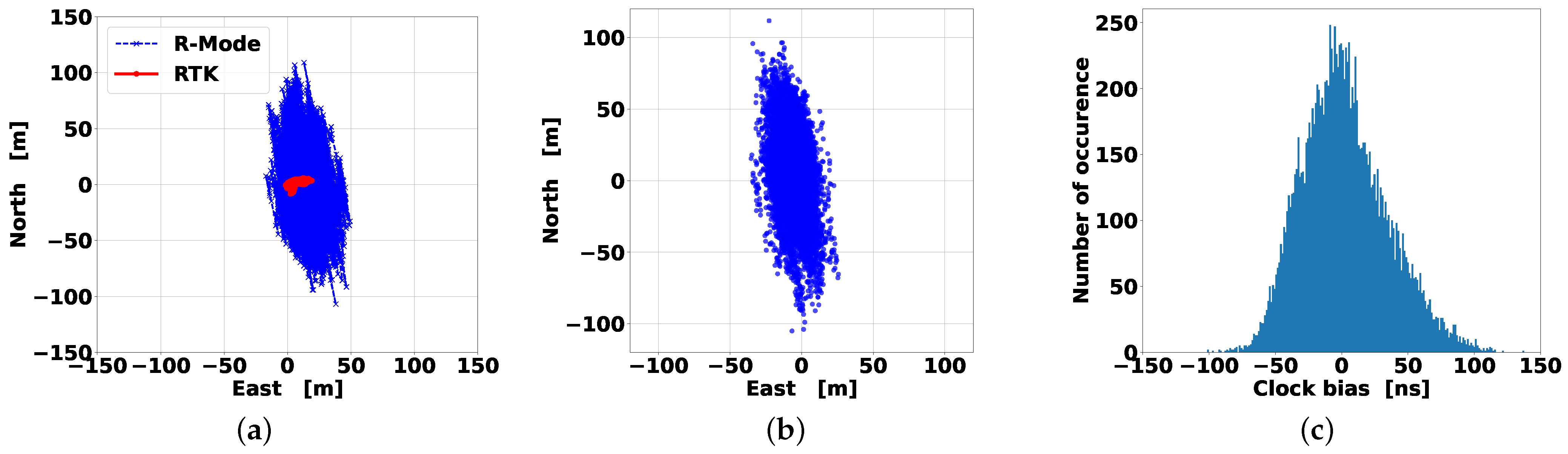
4.2. Night-Time Results

The night-time data presented in this section was recorded between 2:05 UTC and 6:00 UTC on 22 September. As for the daytime scenario, Table 3 contains the information on the usable signals. It appears clear that the stations far away from the receiver, Hoburg, Rozewie and Holmsjö, were set as unhealthy due to the large error introduced by the sky-wave interference. Moreover, the CW2 of Groß Mohrdorf was also set as unhealthy due to the observed signal instability.
The R-Mode position solution was compared with the GNSS RTK reference track, as shown in Figure 8a in a local east-north coordinate system. It can be noted that the ship kept its position almost stable overnight. Therefore, we can think of this test as a semi-static case with a very limited position variation of the ship, in the order of 20 m, and induced by the wind and waves.
The scatter of the R-Mode solution is presented in Figure 8b, where it is clear that the DOP plays an important role in this case. In fact, as mentioned before, only three stations were used to solve the navigation equation, and this increased the overall DOP. The east DOP and north DOP increased to 1.3 and 4.9, respectively, whereas the HDOP reached a value of 5.0. Thus, a loss in the performance level is expected. The 95th quantile accuracy for this data set is 55.3 m, which again satisfies the requirements for coastal navigation, as stated in the previous section. Last but not least, the accuracy of the time estimation is given in the histogram represented in Figure 8c. By comparing this histogram with the one in Figure 7c, we can clearly observe the decrease in the timing accuracy. In particular, the overall bias of 2.3 ns improves, but the standard deviation of 32.3 ns increases by a factor of 3, approximately.
In order to see the sky-wave effect on the ranging performance, the unbiased normalized distribution of the range error for the CW1 of all the transmitters is shown in Figure 9, for daytime and night-time. Looking at the Groß Mohrdorf plot (Figure 9a), a small difference between the daytime and night-time distributions is visible. Surprisingly, the standard deviation for the daytime range error is slightly higher (3.0 m) than the night-time one (1.7 m). Our hypothesis to explain this unexpected result is that the daytime accuracy is somewhat degraded by the AGDF impact. Additionally, there might be a difference between daytime and night-time atmospheric noise, which can change the carrier to noise-density ratio and, therefore, the accuracy of the phase estimation. Unfortunately, the carrier to noise-density ratio estimation was not available at the time of the campaign. Nevertheless, no sky-wave was expected to be visible for that radio beacon due to the distance of only 62 km.
For Hammerodde (Figure 9b), there is a difference between the daytime standard deviation, 5.9 m, and the night-time one of 8.3 m. In this case, a decrease in the accuracy was expected due to the greater distance of about 212 km between the receiver and transmitter. The sky-wave impact is remarkably visible for Helgoland (Figure 9c), located at a distance of 267 km. It can be noted how the night-time distribution spreads much more than the daytime distribution. In detail, the standard deviation is 6.0 m for the day and 15.3 m for the night.
In Figure 9, we can observe in the lower plots the distribution of the error for the stations which were not used in the navigation solution, i.e., Hoburg (Figure 9d), Holmsjö (Figure 9e) and Rozewie (Figure 9f). It is important to note that a different scale is used on the horizontal axis with respect to the upper plots. It appears clear that the error at night is significantly larger than during the day. We can deduce that the sky-wave also depends on the distance between the transmitter and the receiver. In general, at larger distances the ground-wave is more attenuated than the sky-wave, which introduces larger errors. Moreover, the attenuation of the ground-wave depends on the propagation path, as explained in Section 3.1. Therefore, a signal which travels mostly over land will be attenuated more than a signal travelling over water. This effect explains the larger difference in range accuracy between Hammerodde and Helgoland. Despite the fact that the distance from each of them to the receiver is similar, the signal from Helgoland travels mostly over land, whereas the one from Hammerodde travels mostly over water, as is visible in Figure 6.

5. Conclusions

This paper presents a detailed description of the MF R-Mode system, as implemented in the Baltic Sea. Eight radio beacons around the southern Baltic Sea are able to provide the R-Mode as an additional service for testing and development in order to support safe navigation at sea.
The system presents three challenges which are addressed in the paper. The ground wave, which is the expected propagation path for the R-Mode signal, is affected by different propagation velocities depending on type of land and water (fresh, sea). The effect can be modeled or measured.
Secondly, during the night, a reflection of the transmitted signal at the E-layer of the ionosphere comes into effect, which causes a degradation of the R-Mode performance due to the interference with the ground-wave at the receiver site. The sky-wave interference was modeled in the paper and analyzed with respect to the impact on the received signal amplitude phase and the phase error compared to the ground-wave. This model enabled the calculation of the maximum error that can be expected during sky-wave conditions. In the future, this model could also be used to calculate the expected sky-wave impact, taking into account the statistics of the expected sky-wave amplitudes and delays.
The third challenge is some features of the R-Mode signals that can be observed in the transmissions from different stations, which seem to have a technical cause. They appear as jumps in the phase by several meters from one second to the next, which makes it possible to detect them. For now, the affected signals are not used.
The performance of the MF R-Mode system in the testbed area close to Rostock was presented in terms of horizontal positioning and timing accuracy. We demonstrated that good accuracy can be achieved during the day, whereas the problem of the sky-wave multipath degrades system performance at night. In this contribution, we have been able to confirm that the R-Mode could be a suitable backup system for the maritime domain. In particular, the 95% horizontal accuracy achieved was 15.1 m for 6 h during the day and 55.3 m for 4 h at night. In both cases, the accuracy requirement of 100 m for coastal navigation was met over the time slots considered.
Furthermore, we found that at night, no sky-wave disturbance is visible for a distance of up to 62 km. For distances of 210 km to 270 km, the composition of the propagation path is important. On a nearly complete over-sea path, the sky wave has a low impact. The R-Mode signal shows a low degradation. For propagation half over sea and half over land, the standard deviation error increased by a factor of 2.6. In the future, this knowledge could be used to design an adaptive filter for weighting the different measurements in the positioning algorithm at night to provide measurements with an expected higher probability of the sky-wave with less weight.
In general, predicting the effect of the sky-wave can be very challenging due to its dependency on solar activity. Different performance levels might be experienced by the users on different days, during different seasons or at different times of the day. Therefore, the correct modelling of the sky-wave interference effect on phase estimation may be an interesting area of research, given the large number of parameters to be considered in the model itself. For the moment, a working solution is to detect the sky-wave by a stronger variation of the signal amplitude and reduce the service range at night.
Finally, the study of interference mitigation strategies may be an important point of the investigation for the future in order to improve the MF R-Mode system performance at night.

Author Contributions

Conceptualization, F.G.R., L.G. and S.G.; Methodology, F.G.R., L.G. and S.G.; Software, F.G.R., L.G. and S.G.; Validation, F.G.R.; Formal analysis, F.G.R., L.G. and S.G.; Investigation, F.G.R.; Data curation, F.G.R., L.G. and S.G.; Writing—original draft, F.G.R., L.G., S.G. and T.E.; Writing—review & editing, F.G.R., L.G., S.G. and T.E.; Visualization, F.G.R.; Project administration, S.G.; Funding acquisition, S.G. All authors have read and agreed to the published version of the manuscript.

Funding

This research received no external funding.

Institutional Review Board Statement

Not applicable.

Informed Consent Statement

Not applicable.

Data Availability Statement

Not applicable.

Acknowledgments

This research was conducted within the framework of the R-Mode Baltic project, which aims to set up the first combined MF and VDES R-Mode testbed in the southern Baltic Sea and demonstrate that the R-Mode fulfils the maritime user requirements. The authors thank the entire R-Mode Baltic project team. Furthermore, the authors thank the European Union for co-financing the R-Mode Baltic project through the European Regional Development Fund within the Interreg Baltic Sea Region Programme.

Conflicts of Interest

The authors declare no conflict of interest.

Abbreviations

The following abbreviations are used in this manuscript:
AGDFAtmospheric and Ground Delay Factor
APNTAlternative Position, Navigation and Timing
BSHGerman Federal Maritime and Hydrographic Agency
CWContinuous Wave
DGNSSDifferential Global Navigation Satellite System
DLRGerman Aerospace Center
DOPDilution Of Precision
FDMAFrequency Division Multiple Access
FFTFast Fourier transform
GNSSGlobal Navigation Satellite system
GPSGlobal Positioning System
GSARGround-wave-to-Sky-wave Amplitude Ratio
HDOPHorizontal Dilution Of Precision
IALAInternational Association of Marine Aids to Navigation and Lighthouse Authorities
ITUInternational Telecommunication Unit
LOSLine-Of-Sight
MFMedium Frequency
MSKMinimum Shift Keying
OSNMAOpen Service Navigation Message Authentication
PNTPosition, Navigation and Timing
R-ModeRanging Mode
RTKReal-Time Kinematic
SDRSoftware-Defined Radio
UTCCoordinated Universal Time
VDESVery High Frequency Data Exchange System

Appendix A

The section shows the derivation of the formulas used in the paper. As is well-known, the sum of two sinusoidal signals with the circular frequency ω = 2 π f is also a sinusoidal signal with the same frequency. By using the trigonometric addition formulas, we define the two sinusoids, as follows
s 1 ( t ) = A 1 cos ( ω t + θ 1 ) = A 1 cos ω t cos θ 1 sin ω t sin θ 1
and
s 2 ( t ) = A 2 cos ( ω t + θ 2 ) = A 2 cos ω t cos θ 2 sin ω t sin θ 2 .
Then the sum is given as
s 3 ( t ) = s 1 + s 2 = cos ( ω t ) [ A 1 cos ( θ 1 ) + A 2 cos ( θ 2 ) ] sin ( ω t ) [ A 1 sin ( θ 1 ) + A 2 sin ( θ 2 ) ] .
Our goal is to find amplitude A 3 and phase θ 3 of s 3 . We define, as follows
A 3 cos ( θ 3 ) = A 1 cos ( θ 1 ) + A 2 cos ( θ 2 )
and
A 3 sin ( θ 3 ) = A 1 sin ( θ 1 ) + A 2 sin ( θ 2 ) .
Substituting Equations (A4) and (A5) in Equation (A3) and by knowing the trigonometric addition formula, we obtain
s 3 = A 3 [ cos ( ω t ) cos ( θ 3 ) sin ( ω t ) sin ( θ 3 ) ] = A 3 cos ( ω t + θ 3 ) .
To derive the formula which shows the dependency of A 3 on amplitude and phase of s 1 and s 2 , we square and sum Equations (A4) and (A5). After some passages, we obtain
A 3 = A 1 2 + A 2 2 + 2 A 1 A 2 cos ( θ 1 θ 2 ) .
To find θ 3 , we divide Equation (A5) by (A4), obtaining
tan ( θ 3 ) = A 1 sin ( θ 1 ) + A 2 sin ( θ 2 ) A 1 cos ( θ 1 ) + A 2 cos ( θ 2 ) .
By inverting Equation (A8), we can write θ 3 , as follows
θ 3 = tan 1 A 1 sin ( θ 1 ) + A 2 sin ( θ 2 ) A 1 cos ( θ 1 ) + A 2 cos ( θ 2 ) .
We are now interested in the maximum phase error caused by the signal s 2 when it is summed to s 1 . For simplicity, we assume θ 1 = 0 . Therefore, the phase error is directly represented by θ 3 . To find the maximum, we compute the first derivative of Equation (A9) and find the zeros. We first define the ratio between A 1 and A 2 as ρ and then, remembering that θ 1 = 0 , we write Equation (A9), as follows
θ 3 = tan 1 sin ( θ 2 ) ρ + cos ( θ 2 ) .
We also assume ρ > 1 , which means A 1 > A 2 . Then, we compute the derivative with respect to θ 2
d θ 3 d θ 2 = 1 1 + sin θ 2 ρ + cos θ 2 2 cos θ 2 ( ρ + cos θ 2 + sin 2 θ 2 ) ( ρ + cos θ 2 ) 2 = ( ρ + cos θ 2 ) 2 ( ρ + cos θ 2 ) 2 + sin 2 θ 2 cos θ 2 ( ρ + cos θ 2 + sin 2 θ 2 ) ( ρ + cos θ 2 ) 2 = ρ cos θ 2 + cos 2 θ 2 + sin 2 θ 2 ρ 2 + 2 ρ cos θ 2 + cos 2 θ 2 + sin 2 θ 2 = 1 + ρ cos θ 2 ρ 2 + 2 ρ cos θ 2 + 1
from which we find
cos θ 2 = 1 / ρ θ 2 = arccos ( 1 / ρ ) .
Substituting Equation (A12) in (A10), we obtain
θ 3 = tan 1 sin [ arccos ( 1 / ρ ) ] ρ + cos [ arccos ( 1 / ρ ) ] = tan 1 1 1 ρ 2 ρ 1 ρ = tan 1 1 ρ 2 1 .
By observing Equation (A13), it can be noted that the maximum error depends purely on the ratio ρ . This formula cannot be applied if 0 < ρ 1 . In such a case, we consider the four-quadrant arctangent instead of the normal arctangent operator. Thus, Equation (A10) becomes
θ 3 = atan 2 ( sin θ 2 , ρ + cos θ 2 )
from which it is easy to deduce that the worst case coincides with θ 2 = ± π , which results in θ 3 = ± π . To be precise, π is not included in the domain and we should say that for θ 2 π , θ 3 π .

References

  1. EUSPA. EUSPA EO and GNSS Market Report; Technical Report; Publications Office of the European Union: Luxembourg, 2022; Issue 1. Available online: https://data.europa.eu/doi/10.2878/94903 (accessed on 21 December 2022).
  2. Volpe, J.A. Vulnerability Assessment of the Transportation Infrastructure Relying on Global Positioning System; Technical Report; Volpe National Transportation System Center: Cambridge, MA, USA, 2001.
  3. The Royal Accademy of Engineering. Global Navigation Space Systems: Reliance and Vulnerabilities; Technical Report; The Royal Accademy of Engineering: Edinburgh, UK, 2011. [Google Scholar]
  4. Dovis, F. GNSS Interference Threats and Countermeasures; Artech House: Norwood, MA, USA, 2015. [Google Scholar]
  5. EUSPA. Galileo Open Service Navigation Message Authentication (OSNMA): Info Note; Technical Report; Publications Office of the European Union: Luxembourg, 2021. Available online: https://data.europa.eu/doi/10.2878/49446 (accessed on 21 December 2022).
  6. Gewies, S.; Dammann, A.; Ziebold, R.; Bäckstedt, J.; Bronk, K.; Wereszko, B.; Rieck, C.; Gustafson, P.; Eliassen, C.G.; Hoppe, M.; et al. R-Mode testbed in the Baltic Sea. In Proceedings of the 19th IALA Conference, Incheon, Republic of Korea, 27 May–2 June 2018. [Google Scholar]
  7. Johnson, G.; Swaszek, P. Feasibility Study of R-Mode Using MF DGPS Transmissions; Technical Report; ACCSEAS Project: St Germain en Laye, France, 2014. [Google Scholar]
  8. Johnson, G.; Swaszek, P. Feasibility Study of R-Mode Using AIS Transmission: Investigation of Possible Methods to Implement a Precise GNSS Independent Timing Signal for AIS Transmission; Technical Report; ACCSEAS Project: St Germain en Laye, France, 2014. [Google Scholar]
  9. Johnson, G.; Dykstra, K.; Ordell, S.; Swaszek, P. R-Mode Positioning System Demonstration. In Proceedings of the 33rd International Technical Meeting of the Satellite Division of The Institute of Navigation (ION GNSS+ 2020), St. Louis, MO, USA, 22–25 September 2020; Volume 202, pp. 839–855. [Google Scholar] [CrossRef]
  10. Johnson, G.W.; Swaszek, P.F.; Hoppe, M.; Grant, A.; Safar, J. Initial Results of MF-DGNSS R-Mode as an Alternative Position Navigation and Timing Service. In Proceedings of the 2017 International Technical Meeting of The Institute of Navigation, Monterey, CA, USA, 30 January–2 February 2017; pp. 1206–1226. [Google Scholar] [CrossRef] [Green Version]
  11. Yu, J.; Rhee, J.H. Simulation of Medium-Frequency R-Mode Signal Strength. In Proceedings of the 2022 IEEE International Conference on Consumer Electronics-Asia (ICCE-Asia), Yeosu, Republic of Korea, 26–28 October 2022; pp. 1–3. [Google Scholar] [CrossRef]
  12. Jeong, S.; Son, P.W. Preliminary Analysis of Skywave Effects on MF DGNSS R-Mode Signals During Daytime and Nighttime. In Proceedings of the 2022 IEEE International Conference on Consumer Electronics-Asia (ICCE-Asia), Yeosu, Republic of Korea, 26–28 October 2022; pp. 1–4. [Google Scholar] [CrossRef]
  13. Poppe, D.C. Coverage and Performance Prediction of DGPS Systems Employing Radiobeacon Transmissions. Ph.D. Thesis, Bangor University, Bangor, UK, 1995. [Google Scholar]
  14. Grundhöfer, L.; Rizzi, F.G.; Gewies, S.; Hoppe, M.; Bäckstedt, J.; Dziewicki, M.; Del Galdo, G. Positioning with medium frequency R-Mode. Navigation 2021, 68, 829–841. [Google Scholar] [CrossRef]
  15. Cueto-Felgueroso, G.; Martínez, J.; Blesa, S.; Moreno, G.; López, M.; Nieto, R.; Píriz, R.; Hoppe, M.; Gewies, S.; Callewaert, K.; et al. Galileo Timing for R-Mode—Testing Campaign. In Proceedings of the 35th International Technical Meeting of the Satellite Division of The Institute of Navigation (ION GNSS+ 2022), Denver, CO, USA, 19–23 September 2022; pp. 439–456. [Google Scholar] [CrossRef]
  16. Subirana, J.; Zornoza, J.; Hernández-Pajares, M. GNSS Data Processing Volume I: Fundamentals and Algorithms; ESA Communications: Noordwijk, The Netherlands, 2013. [Google Scholar]
  17. Vincenty, T. Direct and inverse solutions of the geodesics on the ellipsoid with application of nested equations. Surv. Rev. 1975, 23, 88–93. [Google Scholar] [CrossRef]
  18. ITU. Ionosphere and Its Effects on Radiowave Propagation; International Telecommunication Union: Geneva, Switzerland, 1998. [Google Scholar]
  19. Pressey, B.G.; Ashwell, G.E.; Fowler, C.S. The measurement of the phase velocity of ground-wave propagation at low frequencies over a land path. Proc. IEE Part III Radio Commun. Eng. 1953, 100, 73–84. [Google Scholar] [CrossRef]
  20. Rizzi, F.G.; Hehenkamp, N.; Grundhöfer, L.; Gewies, S. Improving MF R-Mode ranging performance with measurement-based correction factors. In Proceedings of the European Workshop on Maritime Systems Resilience and Security, Bremerhaven, Germany, 20 June 2022. [Google Scholar] [CrossRef]
  21. ITU. ITU-R P.832-4 World Atlas of Ground Conductivities; International Telecommunication Union: Geneva, Switzerland, 2015. [Google Scholar]
  22. Rotheram, S. Ground-wave propagation. Part 1: Theory for short distances. IEE Proc. Commun. Radar Signal Process. 1981, 128, 275–284. [Google Scholar] [CrossRef]
  23. Rotheram, S. Ground-wave propagation. Part 2: Theory for medium and long distances and reference propagation curves. IEE Proc. Commun. Radar Signal Process. 1981, 128, 285–295. [Google Scholar] [CrossRef]
  24. Wait, J.R. The ancient and modern history of EM ground-wave propagation. IEEE Antennas Propag. Mag. 1988, 40, 7–24. [Google Scholar] [CrossRef]
  25. Millington, G. Ground-wave propagation over an inhomogeneous smooth earth. Proc. IEE-Part III Radio Commun. Eng. 1949, 96, 53–64. [Google Scholar] [CrossRef]
  26. Grundhöfer, L.; Gewies, S.; Hehenkamp, N.; Del Galdo, G. Redesigned Waveforms in the Maritime Medium Frequency Bands. In Proceedings of the 2020 IEEE/ION Position, Location and Navigation Symposium (PLANS), Portland, OR, USA, 20–23 April 2020; pp. 827–831. [Google Scholar] [CrossRef]
  27. Grundhöfer, L.; Gewies, S. Equivalent Circuit for Phase Delay in a Medium Frequency Antenna. In Proceedings of the 2020 European Navigation Conference (ENC), Dresden, Germany, 23–24 November 2020; pp. 1–6. [Google Scholar] [CrossRef]
  28. Hemisphere. Atlas GNSS Global Correction Service. Available online: https://www.hemispheregnss.com/product/atlas-gnss-global-correction-service/ (accessed on 22 January 2023).
  29. IALA. Recommendation R-129 GNSS Vulnerability and Mitigation Measures, 3.1 ed.; IALA: St Germain en Laye, France, 2012. [Google Scholar]
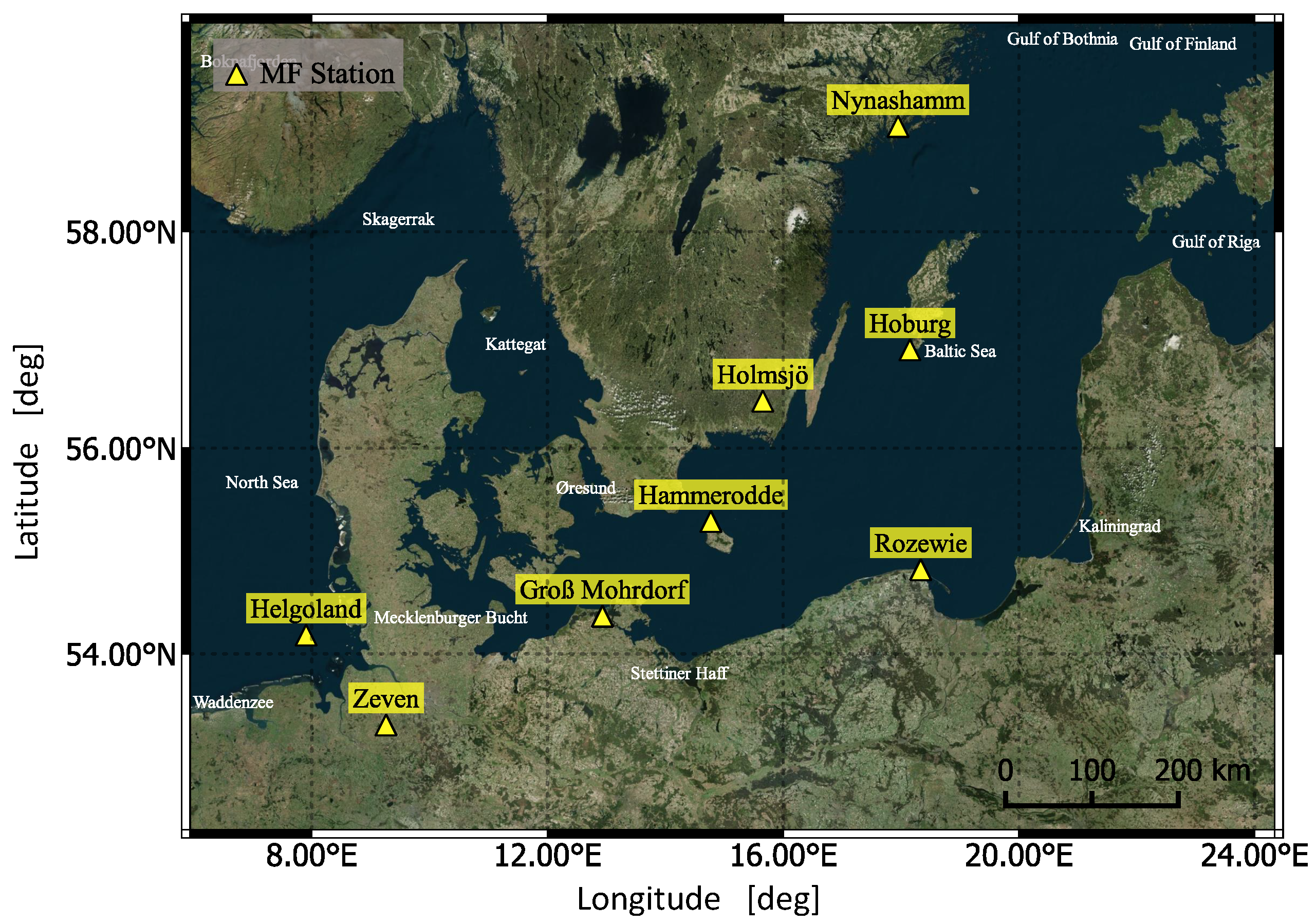
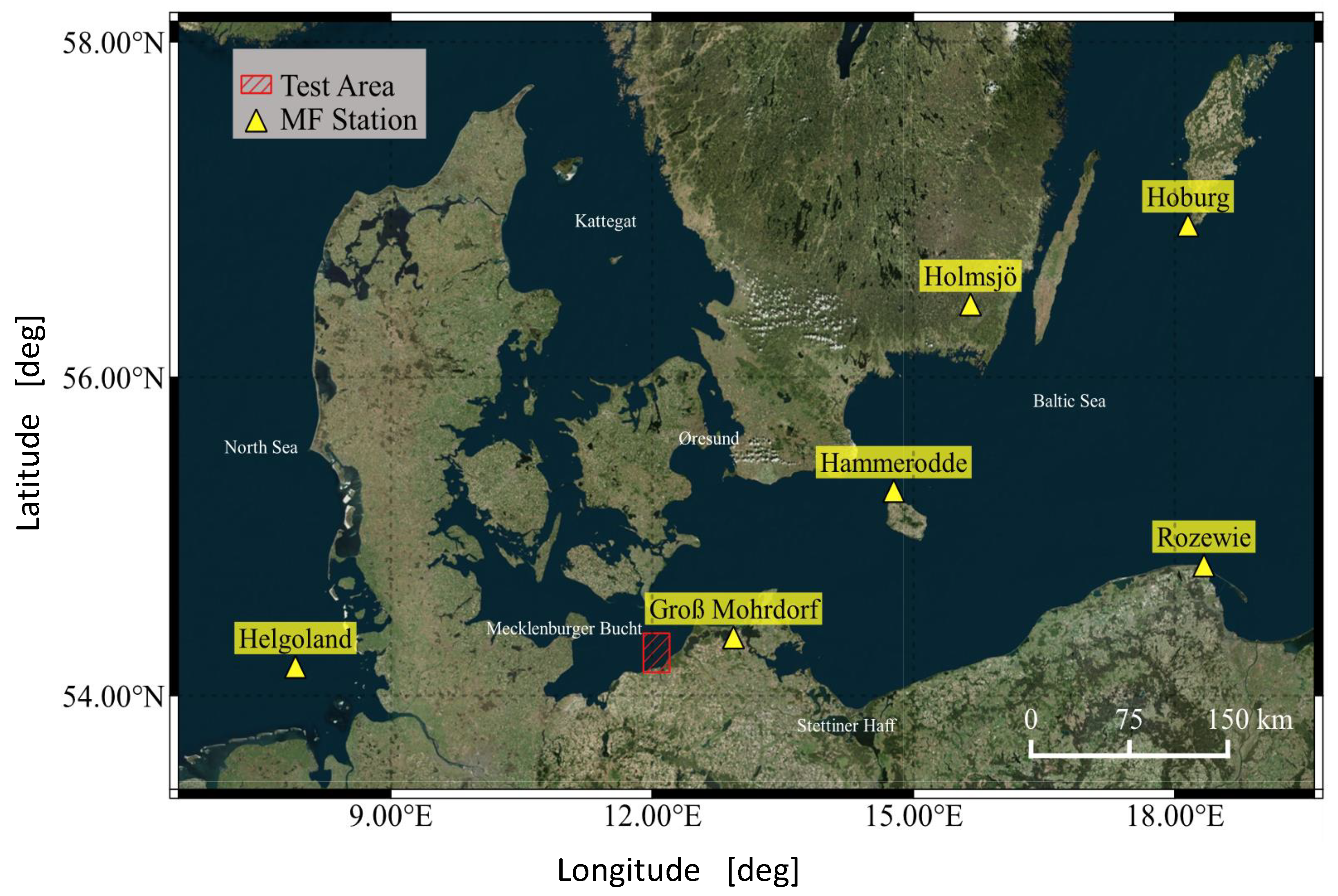
Figure 1. Enabled MF R-Mode radio beacons (yellow triangles) around the southern Baltic Sea.
Applsci 13 01872 g001
Figure 2. Groß Mohrdorf AGDF calculated for the southern Baltic Sea in radians.
Applsci 13 01872 g002
Figure 3. Amplitude (a) and phase error (b) for different GSAR and θ SW .
Applsci 13 01872 g003
Figure 4. Difference between a standard MF radio beacon architecture (above) and the R-Mode-enabled radio beacon (below).
Applsci 13 01872 g004
Figure 5. Instabilities of Groß Mohrdorf radio beacon. The phase error in meter is represented for the two CW signals.
Applsci 13 01872 g005
Figure 6. MF transmitters (yellow triangles) available during the campaign and test area (red rectangle).
Applsci 13 01872 g006
Figure 7. Daytime results. (a) Reference RTK (red circles) and R-Mode (blue crosses) tracks. (b) Scatterplot of the R-Mode positioning error in east and north. (c) Histogram of the estimated receiver clock bias.
Applsci 13 01872 g007
Figure 8. Night-time results. (a) Reference RTK (red circles) and R-Mode (blue crosses) tracks. (b) Scatterplot of the R-Mode positioning error in the east and north. (c) Histogram of the estimated receiver clock bias.
Applsci 13 01872 g008
Figure 9. Normalized range error distribution for the CW1 signal. Solid blue line represents night-time data, while orange dashed line represents daytime data. (a) Groß Mohrdorf. (b) Hammerodde. (c) Helgoland. (d) Hoburg. (e) Holmsjö. (f) Rozewie.
Applsci 13 01872 g009
Table 1. Distance between the transmitters and the centre point of the test area.
Station NameLat [deg]Lon [deg]Distance [km]
Hoburg56.920918.1520486
Rozewie54.830818.3347414
Holmsjö56.444015.6551334
Helgoland54.18597.9052267
Hammerodde55.298114.7738211
Groß Mohrdorf53.374012.934462
Table 2. Daytime: signals used for the position and time estimation in green with the “h” flag. Signals in red with the “uh” flag were not used.
HoburgRozewieHolmsjöHelgolandHammeroddeGroß Mohrdorf
CW1CW2CW1CW2CW1CW2CW1CW2CW1CW2CW1CW2
hhhuhhhhuhhuhhh
Table 3. Night-time signals used for the position and time estimation in green with the “h” flag. Signals in red with the “uh” flag were not used.
HoburgRozewieHolmsjöHelgolandHammeroddeGroß Mohrdorf
CW1CW2CW1CW2CW1CW2CW1CW2CW1CW2CW1CW2
uhuhuhuhhhhhuhuhhuh
Disclaimer/Publisher’s Note: The statements, opinions and data contained in all publications are solely those of the individual author(s) and contributor(s) and not of MDPI and/or the editor(s). MDPI and/or the editor(s) disclaim responsibility for any injury to people or property resulting from any ideas, methods, instructions or products referred to in the content.

