Automatic Detection of Multilevel Communities: Scalable, Selective and Resolution-Limit-Free ^†

Abstract

Community structure is one of the most important features of complex networks. Modularity-based methods for community detection typically rely on heuristic algorithms to optimize a specific community quality function. Such methods have two major limits: (1) the resolution limit problem, which prohibits communities of heterogeneous sizes being simultaneously detected, and (2) divergent outputs of the heuristic algorithm, which make it difficult to differentiate relevant and irrelevant results. In this paper, we propose an improved method for community detection based on a scalable community “fitness function.” We introduce a new parameter to enhance its scalability, and a strict strategy to filter the outputs. Due to the scalability, on the one hand, our method is free of the resolution limit problem and performs excellently on large heterogeneous networks, while on the other hand, it is capable of detecting more levels of communities than previous methods in deep hierarchical networks. Moreover, our strict strategy automatically removes redundant and irrelevant results; it selectively but inartificially outputs only the best and unique community structures, which turn out to be largely interpretable by the a priori knowledge of the network, including the implanted community structures within synthetic networks, or metadata observed for real-world networks.

1. Introduction

Community, also known as a network cluster, is a mesoscopic structure ubiquitous in many real-world systems whose topologies are generally described by complex networks [1]. Since highlighted by Girvan and Newman in 2002 [2], the community structure of a network has been of particular interest to physicists and mathematicians, as it characteristically reveals functional [3,4], relational [1,5,6] or even social information [7,8,9,10,11] of complex systems. Despite certain special definitions of community (for instance, the “disassortative structures,” as studied in [12]), communities are most typically defined as groups of nodes with the connections inside each group being denser than those between different groups [13]. Community detection explores optimized divisions of a network. In previous literature, it has become a standard practice to evaluate the effectiveness of a community detection method by its performances in either recreating the implanted communities in synthetic (i.e., artificial) networks, or recovering observed node attributes or metadata for real-world networks. Properties of communities such as community resilience [14] and community vulnerability [15,16] can be studied afterwards.

To detect the correct communities for a network is always a challenge. Related studies can be traced back all along to “graph partitioning” in graph theory [17], or “hierarchical clustering” in sociology [18,19]. For large graphs, finding an exact solution to a partitioning task has been proven an NP-complete problem [13,17]. In the case of real-world complex networks, it is even harder: the total number of communities is usually unknown [13], the sizes of different communities may differ by orders of magnitude [20], and the overall structure of the whole network is often multilevel or hierarchical [8,20,21]. Community detection methods generally turn to heuristic algorithms for acceptably good solutions [13]. A good many community detection algorithms came out, among which the most well-known ones include spectral clustering [22,23,24], stochastic block models [25,26], modularity-based [13,27,28,29,30] or Hamiltonian-based [31,32,33,34,35,36] optimization methods, and information-based approaches such as Infomap [37]. Within the scope of this paper, we focus on the modularity-based methods. In a broad sense, modularity-based methods assess the validity of each potential network division with a specific community quality function; a heuristic algorithm is then employed to optimize the communities by maximizing this community quality function.

Modularity-based methods, and also Hamiltonian-based methods, have been argued to have two major limits. The first one is the well-known “resolution limit problem” raised by Fortunato and Barthelemy in 2007 [3]. Depending on the numbers of intra connections of communities and the total number of connections within the whole network, a modularity optimization method tends to merge small communities (even if they are well-defined clusters as complete graphs) into larger but sparser ones. This reveals a fact that the modularity-based method cannot find communities of small sizes, much as a microscope cannot find microbes beyond its resolution range. For quality functions other than the modularity, the same phenomenon has also been observed [38]. On the other hand, modularity-based methods may detect unreasonable community structures due to inappropriate resolutions, for example, they detect communities for random graphs [39,40]. In order to overcome the resolution limit, a variety of “multiresolution” methods were suggested. They use a tunable parameter to alter the resolution and detect communities of different levels within different resolution scales [5,30,33,35,41]. However, a further study by Lancichinetti and Fortunato [42] pointed out that the resolution limit problem is actually induced by two opposite tendencies: the tendency of merging small communities, and the tendency of breaking large ones. If the communities within the same network have very different sizes, it becomes impossible for an optimization approach to avoid both biases simultaneously. Multiresolution methods seemed to outperform other methods only because the community sizes used in previous tests were “too close to one another,” spanning less than one order of magnitude [42]. When the community sizes vary over up to two orders of magnitude, as in many real-world networks [20,43], existing multiresolution methods also fail to recover the expected community structures [42].

The second limit of modularity optimization method is that finding an optimal division for any given network is normally infeasible. It has been recognized that the modularity landscape of a network often includes an exponentially growing (with system size) numbers of local maxima [42,44]. These local maxima may all be very close to the global maximum in terms of modularity, but the corresponding divisions of the network can be topologically utterly different from one another [44]. This implies that not only an exactly optimal division for a network is intrinsically unreachable [42], but the available solutions in practice can be largely unreliable. This problem is even more serious for multiresolution approaches: communities detected in “blurring” resolution scales are often incomprehensible and, for all practical purposes, uninformative. Although it has been argued that inquiring which is the “best” or “most relevant” scale of resolution is an ill posed question [5], many methods still manage to find out the most stable communities that can be detected within a persistent range of resolution. The existence of such stable communities is an observed fact [5]: they form strong “plateaus” in the diagram of community numbers versus the resolution scale [35]. It has become popular in previous literature to rank the confidence of detection results by their strengths of plateaus; community structures suggested by strong plateaus have been demonstrated to be frequently consistent with the a priori knowledge about the network [5,30,35].

Nevertheless, existing methods using the stability of plateaus are not yet satisfying. On the one hand, a plateau was originally expected to reflect the multiple times of discovery of exactly the same communities at different resolutions. However, no comparison on the community structure represented by each data point within the same plateau has been explicitly conducted in previous literature, leaving a doubt that the same plateau may not represent the same community structure at all. Some methods, as in [5,45,46], simply define plateaus by the numbers of communities, some by the values of modularity [30], while some others, as in [35], execute quantitative comparisons among the communities detected at fixed resolutions—yet communities detected at different resolutions are still not compared. As discussed in [44], none of such definitions can guarantee each plateau as defined represents an identical community structure. On the other hand, evaluating the stability of plateaus by their lengths is, by far, not sufficient. Although large plateaus are almost always stable [5,30,35], stabilities of small plateaus are uncertain: some of them can be stable and informative, but some others just emerge due to randomness (we will show some examples later). Previous literature either ignores all small plateaus, or artificially selects their preferred ones. Due to these facts, we propose a strict definition for the term “plateau,” as well as an effective strategy to evaluate the stabilities of plateaus, as both are urgently needed.

In this paper, we propose a new approach for multiresolution community detection. We adopt a modified community fitness function [30] and a heuristic Louvain algorithm [47] to find multilevel community structures for complex networks. The innovation of our work includes: (1) we introduce a new scaling factor to enhance the scalability of the community fitness function; (2) we suggest a strict strategy to automatically select the outputs, as well as an explicit definition for the term “plateau,” and (3) we demonstrate our community fitness function is scalable so that it can overcome the resolution-limit problem. To summarize, our approach is scalable, selective, and resolution-limit-free, with clean and inartificial outputs. It performs well on both synthetic benchmark networks and real-world networks.

2. Method

Our method is modularity-based, and multiresolution. It includes three components: (1) a modified community fitness function with a tunable resolution parameter and a scaling factor, (2) a heuristic Louvain algorithm to maximize this community fitness function, and (3) a strategy to filter the output and retrieve the most stable and significant results. Next, we introduce these three components separately; at the end of this section we display the whole framework of our approach.

2.1. Community Fitness Function

The so-called community fitness function was firstly proposed by Lancichinetti and Fortunato [30]. Its original form is as following [30]:

$$f^{\mathcal{G}}=\frac{k_{in}^{\mathcal{G}}}{{(k_{in}^{\mathcal{G}}+k_{out}^{\mathcal{G}})}^{\alpha }}$$

(1)

Here, $\mathcal{G}$ denotes a community given by a certain network division, $f^{\mathcal{G}}$ quantifies the fitness (i.e., quality) of community $\mathcal{G}$: larger values of $f^{\mathcal{G}}$ indicate more reliable communities. $k_{in}^{\mathcal{G}}$ and $k_{out}^{\mathcal{G}}$ in the formula stand for the in-degree and out-degree of community $\mathcal{G}$, defined in the same way as those in previous literature, such as [8]. α (α > 0) is a resolution parameter that tunes the resolution: large values of α yield small communities, while small values of α deliver large communities [30].

Instead of the widely-used modularity function Q proposed by Newman [13,48], we choose to use the community fitness function because it is, by design, scalable and is promising to avoid the resolution limit problem. Its original form, as in Formula (1), can be directly used in our method; actually, we do use it in many of our calculations in the following part of this paper. Yet, for networks that have multilevel or hierarchical structures, it would be helpful to introduce an additional parameter β to rescale the varying range of the resolution parameter α. In this paper, we suggest a modified form of $f^{\mathcal{G}}$ as

$${\left(f_{\alpha }^{\beta }\right)}^{\mathcal{G}}=\frac{{(k_{in}^{\mathcal{G}})}^{\beta }}{{(k_{in}^{\mathcal{G}}+k_{out}^{\mathcal{G}})}^{\alpha }}.$$

(2)

Here, the power exponent β (β ≥ 1) is our newly introduced “scaling factor;” when β = 1, Formula (2) degrades to Formula (1). When detecting communities with ${\left(f_{\alpha }^{\beta }\right)}^{\mathcal{G}}$, we search for an optimized division of the network that maximizes the summative fitness of all detected communities:

$$F_{\alpha }^{\beta }={\displaystyle \sum _{\mathcal{G}}{\left(f_{\alpha }^{\beta }\right)}^{\mathcal{G}}}={\displaystyle \sum _{\mathcal{G}}\frac{{(k_{in}^{\mathcal{G}})}^{\beta }}{{(k_{in}^{\mathcal{G}}+k_{out}^{\mathcal{G}})}^{\alpha }}}$$

(3)

Alternatively, maximizing the average fitness (i.e., $F_{\alpha }^{\beta }$ divided by the total number of communities), as in [30], also yields essentially equivalent results.

The scaling factor β amplifies the varying range of the resolution parameter α. For each fixed β, we estimate in Appendix A that the varying range of α should be between β − 1 and 2β − 1: α < 2β − 1 prevents unexpected splitting of large communities, while α > β − 1 avoids inappropriate merging of small communities. For example, random graphs exhibit no community structure within this resolution scale, and dense clusters that are sparsely connected will not merge into one large community. Obviously, when β = 1, α should vary between 0 and 1; when β > 1, the varying range of α has been amplified β times.

In practice, for networks having only one single community level, varying α within (β − 1, 2β − 1) is already sufficient for the expected communities being detected. However, for networks with multiple community levels, within range (β − 1, 2β − 1), only communities of the lowest level (i.e., communities of smallest sizes that cannot split further) can be detected. This is because higher levels of communities come from combinations of lower-level communities; to allow such combinations, the lower bound β − 1 must be relaxed. Therefore, in our calculation we run our algorithm with the resolution parameter α varying between 0 and 2β − 1, which enables us to detect multiple levels of communities within different resolution scales.

2.2. Heuristic Optimization Algorithm

Since optimizing a community quality function has been proven an NP-complete problem [13,17], heuristic algorithms are generally adopted to obtain the best available solutions. Early methods, such as those in [2,13], usually have heavy demands on computational resources, while more recently, a number of faster algorithms have been proposed [27,43,47,48,49]. Among them, the Louvain algorithm proposed by Blondel et al. [47] is widely accepted due to its prominent efficiency and high accuracy. The label “Louvain” comes from the authors’ affiliation (UCLouvain); alternatively, it is also called a “BGLL” algorithm, by the authors’ initials. Originally, this algorithm was designed as a greedy algorithm to optimize the standard modularity function Q proposed by Newman [48]; similar algorithms have also been adopted to optimize the Potts Hamiltonian by some dynamical methods [35,36].

We employ the Louvain algorithm to optimize our community fitness function (Formula (3)) in this paper. Here, we briefly describe its steps; for more details, please refer to [47].

• Initialize communities. At the very beginning, each node of the network is designated to an individual community. A network consisting of N nodes is then divided into N communities of size 1.
• Optimize communities of the lowest level. Sequentially consider each node of the network and scan its neighboring communities (i.e., communities sharing at least one edge with the node in focus). Calculate the potential gains of $F_{\alpha }^{\beta }$ if the node in focus was moved out of its original community and put into each of the neighboring communities. Place the node in focus into the community that leads to a maximum value of $F_{\alpha }^{\beta }$.
• Iterate until convergence. Repeat step 2 until a maximum value of Formula (3) is reached where no more moves of any node may further increase this value. During this process, the sequence of node orders is randomized every time a new round of iteration is started.
• Merge communities to build a higher community level. Consider each community obtained at the convergence of step 3 as a fixed module; hereafter, all its members (nodes) must be moved together. Repeat the above steps 2 and 3 by taking each fixed module as a node. During this process, connected modules gradually condense into communities of higher levels, until a maximum value of Formula (3) is reached.
• Iterate until convergence at the highest level. Repeat step 4 and detect communities of all levels, until the highest level is detected where no further merging of any communities can increase $F_{\alpha }^{\beta }$.
• Output communities. Communities of all levels detected by the above steps 1 to 5 form a hierarchical structure; each level can be independently outputted. Customarily, only the output of the highest level is adopted since it has a maximum value of $F_{\alpha }^{\beta }$ among all levels.

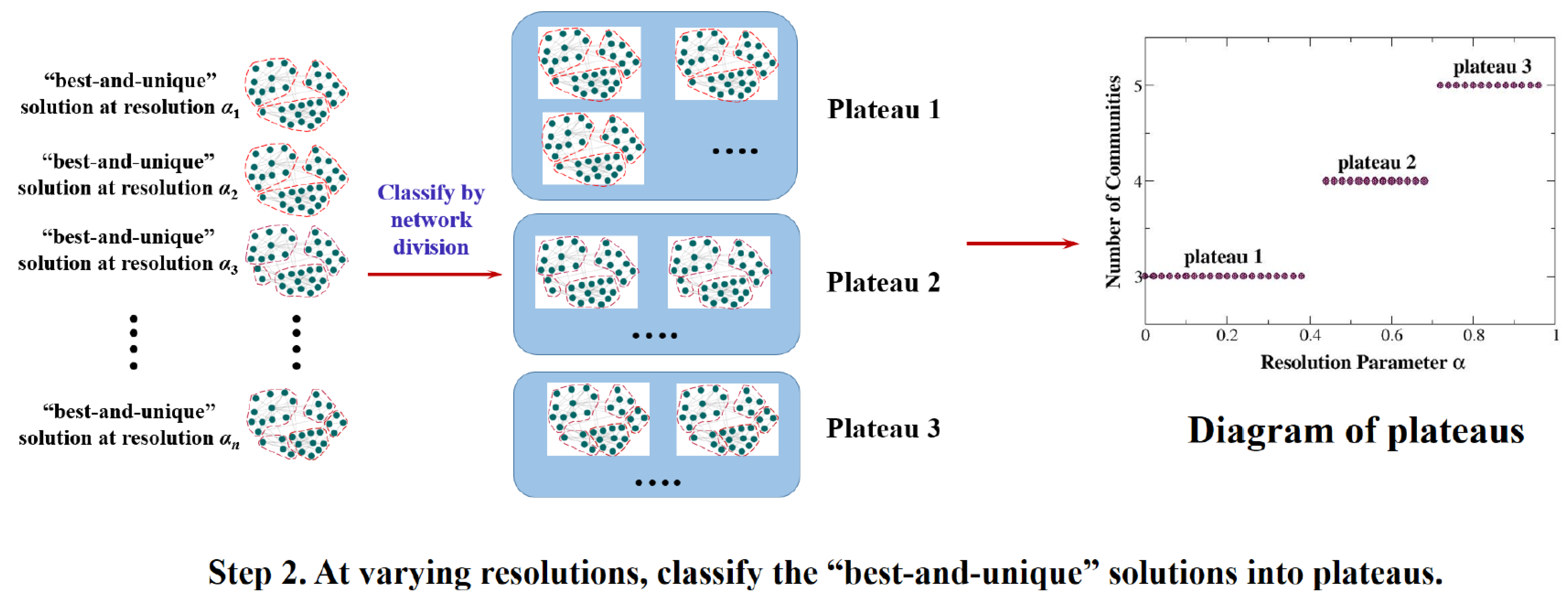
2.3. Strategy to Filter the Output

We adopt a strict filtering strategy to ensure the selectivity of our method. As a heuristic approach, the Louvain algorithm optimizing our community fitness function often converges to different solutions in different realizations. Many of these solutions are “local maxima”, which emerge only by chance. To retrieve from messy outputs the most relevant solutions that can be persistently detected, previous methods customarily rely on the stability of plateaus [5,30,35,44,45,46], only the term “plateau” was, so far, everywhere loosely defined (see our arguments in the Introduction). In this section, we suggest a much stricter definition for plateaus and, correspondingly, a strict strategy to identify them. By our definition, a plateau is a continuous scale of resolution within which the best solutions found by a heuristic optimization algorithm uniformly converges to an identical topological structure of community. To detect such plateaus, it is required to compare not only the topologies of solutions obtained at each fixed resolution, but also those at different resolutions. We suggest the following strategy to discover our plateaus:

• At each fixed resolution (i.e., with fixed values of parameters α and β), we implement the Louvain algorithm on the same network in multiple realizations. Among the outputs of all realizations, we adopt the ones with the highest value of $F_{\alpha }^{\beta }$ as our best solutions obtained at this resolution. In addition, we require the topology of these best solutions to be unique: in case two or more solutions have equally highest values of $F_{\alpha }^{\beta }$, but represent different topological structures of community, all solutions obtained at this resolution will be abandoned, and the corresponding resolution will be considered “irrelevant” and not contributing to any potential plateau.
• At different resolutions, with varying values of α (during which the value of β is still fixed), we run the above step 1 and obtain the best-and-unique solutions at all relevant resolutions. Then we compare the topologies of these best-and-unique solutions, and classify them into different plateaus; solutions classified to the same plateau must represent exactly the same topological structure of community.

The above step 1 compares the topologies of communities detected at each fixed resolution. We require topological uniqueness of all our best solutions because otherwise they might be the results of randomness due to the Louvain heuristic; below, we will show some examples. Step 2 compares the topologies of the best-and-unique solutions obtained at varying resolutions. Plateaus defined and identified as above strictly fulfil “one plateau, one topological structure of community”. Our strict strategy guarantees such plateaus are truly stable, since random outputs of the algorithm have all been filtered out. Only then can the stability (or say, “robustness”) of solutions be measured by the lengths of their corresponding plateaus. It is common in previous literature [5,30,35,44,45,46] to either take the communities detected by the longest plateaus as the most relevant results, or artificially select favored structures that best fit the a priori knowledge about the network. To our viewpoint, all best-and-unique solutions represented by the our strictly-defined plateaus should have their own particular information: they discover different structures that represent different aspects of the given network. Thus in this paper, we do not select plateaus simply by their lengths. Instead, we output and interpret “only the stable plateaus, and all the stable plateaus”.

Figure 1 shows the whole framework of our proposed approach, with all the three components discussed above settled in place.

3. Results

In this section, we firstly demonstrate the effectiveness of our approach in recovering implanted community structures for synthetic benchmark networks, including multilevel communities within hierarchical networks (Section 3.1), and communities of distinct sizes in heterogeneous networks (Section 3.2). Then, we apply our method to some well-studied real-world networks, exhibiting both its consistency and discrepancy with the observed node attributes or metadata (Section 3.3). Finally, we implement our algorithm to certain extremely large networks with ground truth communities to test its performance as the network’s size increases (Section 3.4).

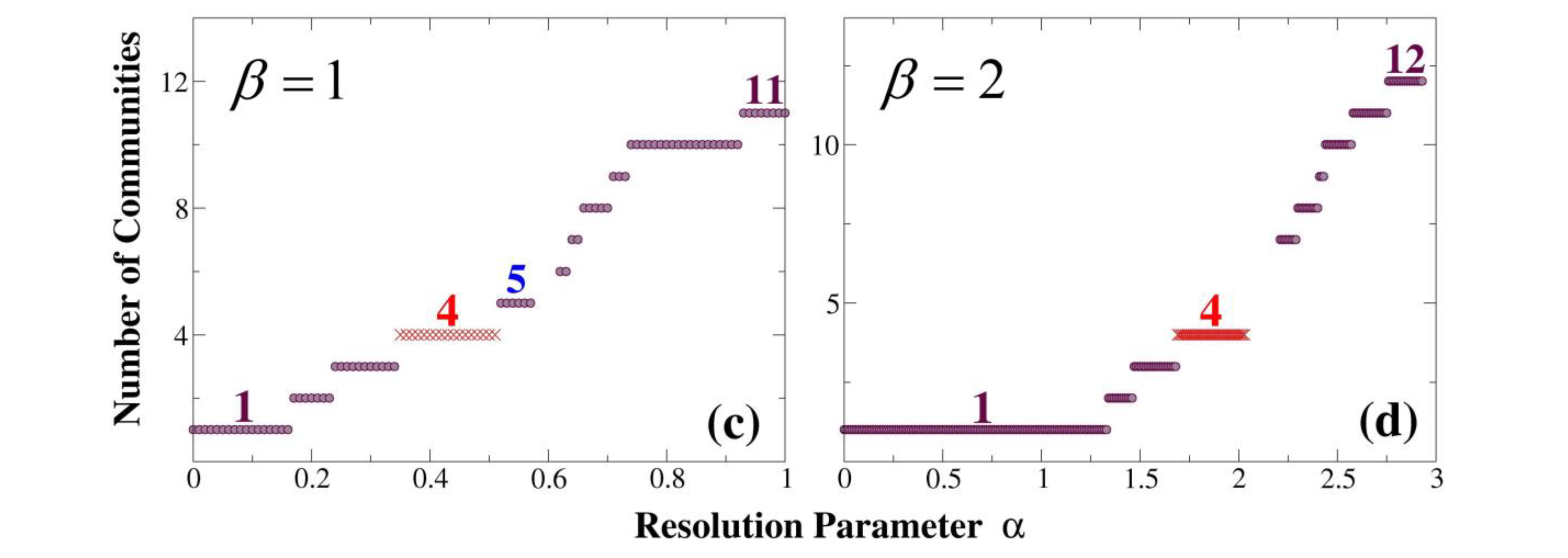
3.1. On the Hierarchical Ravasz-Barabasi (RB) Networks

We first of all introduce the structure of the Ravasz–Barabasi (RB) networks [20]. The smallest RB network is RB5, which is a complete graph consisting of 5 nodes and 10 edges, see Figure 2a. To facilitate our discussion, we call node 0 the central node, while all other nodes are peripheral nodes of the RB5 network. RB5 is a basic unit to constitute larger RB networks. Five RB5 units, one in the center and four on the periphery, constitute an RB25 network, as shown in Figure 2b,c. According to [20], these RB5 units should be connected in such a way: every peripheral node of the peripheral RB5 units is connected to the central node of the central RB5 unit, but the peripheral RB5 units themselves are not connected to one another. Note that in Figure 2b,c, for easy drawing we did not shift the central node of each RB5 unit slightly off its center as in Figure 2a: each RB5 unit in Figure 2b,c is still a complete graph containing 10 edges, only the diagonal edges are invisible by overlapping with other edges. Following the same way, five RB25 units constitute an RB125 network, as shown in Figure 3. Obviously, the RB networks are fractal-like and hierarchical, which can grow infinitely. We choose these networks to test our method because they can provide hierarchical structures of any depth—deep enough to test the limit of any multiresolution method for community detection.

As synthetic/artificial networks, the implanted community structures within the RB networks are apparent: an RB network with 5ⁿ nodes (hereafter, we call it an “RB5ⁿ network”) is expected to be naturally divided into 5ⁿ⁻¹ RB5 units on the lowest community level, or 5ⁿ⁻² RB25 units on a higher level, and so on, constructing a hierarchical structure of n levels. However, such “natural” divisions should not be taken for granted. One problem is, within each RB5^m unit (2 ≤ m ≤ n), the central node (e.g., see the hollow red circles in Figure 2c and Figure 3b–d is connected to every peripheral node of the same unit. By the natural division, this central node always has a larger out-degree than in-degree (for example, the central node of an RB25 network, as in Figure 2b, has an out-degree of 16 but an in-degree of 10), which violates the customary definition of community in a strong sense [50]. Moreover, within larger networks, this problem gets even more serious: when n ≥ 3 the natural division further violates the definition of community in a weak sense [50]. Figure 3a shows an example: the central RB5 community (solid red circles) within an RB125 network has a total out-degree of 80 (all contributed by its central node), but a total in-degree of only 20. Therefore, it seems reasonable to break up the central RB5 community and segregate its central node as an individual community, as we did in Figure 2c, which has also been suggested previously by [4].

Through literature investigation (such as on [4]), as well as numerical simulation, for the RB networks, we propose a plausible revision to their “natural divisions”, i.e., on each community level, preserve the peripheral communities, but further divide the central communities. More specifically, on the lowest community level, instead of 5 communities (as in Figure 2b), we divide each RB25 unit into 6 communities (as in Figure 2c). Thus, an RB5ⁿ network (n ≥ 2) will be divided into 6 × 5ⁿ⁻² communities (since it contains 5ⁿ⁻² RB25 units); Figure 3b shows an example that an RB125 network is so divided into 30 communities. Similarly, on a higher level, we find each RB125 unit tends to split into 10 communities as in Figure 3c: 4 peripheral RB25 units make 4 communities, while the central RB25 unit splits to 6 communities as in Figure 2c. On this level, an RB5ⁿ network (n ≥ 3) will be divided into 10 × 5^{n − 3} communities. Following this regulation, on the m-th community level (2 ≤ m ≤ n, here m = 1 stands for the lowest level), it is each RB5^m+1 unit that splits into 4 m + 2 communities, thus, an RB5ⁿ network (n ≥ m + 1) will be divided into (4 m + 2) × 5^n−m−1 communities. Supplementary Figure S1a visualizes an RB625 network being divided into 14 communities on the third community level, and

Table 1. Numbers of communities on different community levels in our proposed divisions for the RB networks. Here, m = 1 stands for the lowest community level, which divides the network into smallest communities that cannot split further; m is restricted to be no larger than n. Numbers in this table all follow our proposed formula: (4m + 2) × 5^n−m−1. Our method detects all levels of communities when the network is not extremely large (n ≤ 5). When n = 6 (an RB15625 network), the second and fifth levels, which are expected to contain 1250 and 22 communities, turn out to be undetectable by our method.

RB5n Networks	Community Levels (m)
	1 (Lowest)	2	3	4	5	6
RB25 (n = 2)	6	1	/	/	/	/
RB125 (n = 3)	30	10	1	/	/	/
RB625 (n = 4)	150	50	14	1	/	/
RB3125 (n = 5)	750	250	70	18	1	/
RB15625 (n = 6)	3750	1250 (undetectable)	350	90	22 (undetectable)	1

summarizes the numbers of communities on different levels of the RB networks given by the above divisions. Next, we demonstrate how such divisions would be discovered by our method.

We first try with β = 1, i.e., the original form of the community fitness function (Formula (1)). For all RB networks, with β = 1, we only detect two community levels: the highest (but trivial) level that merges the whole network into one single community, and the lowest level that divides the network into smallest communities that cannot split further; intermediate levels, if exist, are all missed. On the other hand, with β = 1, we detect different divisions for the lowest level. Except for our proposed divisions as listed in the first column of Table 1, we also detect the natural divisions, but only for two small RB networks: RB25 and RB125 (see Figure 2b and Figure 3a); for larger RB networks, the natural divisions can no longer stand, since they violate the customary definitions of community too seriously. Moreover, with β = 1, an RB125 network can be divided into 26 communities—this can be done by breaking up only the central RB5 community of each RB125 unit (rather than each RB25 unit) into 2 communities, but preserving all other RB5 communities (as in Figure 3d). Compared to the divisions listed in Table 1, this alternative division can be understood as a result of a “relaxed stringency”, with which an RB5ⁿ network (n ≥ 3) can be divided into 26 × 5ⁿ⁻³ communities; this explains the plateaus representing 26, 130, 650 and 3250 communities that emerge in Figure 3e and Supplementary Figures S1b and S2a,c. Since all these plateaus have similar community sizes (≤5), we classify them all to the lowest community level. Moreover, with an even further relaxed stringency, where only the central RB5 community of each RB625 unit is broken up into 2 communities, an RB625 network can be divided into 126 communities. Yet such stringency has been over-relaxed so that it only produces a very tiny plateau for the RB625 network in Supplementary Figure S1b, but has not been observed anywhere else.

The above results detected with β = 1 are still not satisfying; one major problem is that the highest and lowest community levels have occupied almost all the resolution scales; intermediate levels are seriously compressed and cannot be observed at all. To fix this problem, we take β ≥ 2. It turns out, that with β ≥ 2 our method discovers all community levels including the intermediate ones for the RB networks; see Figure 2e and Figure 3f, Supplementary Figures S1c and S2b for the plateaus obtained with β = 2. With β > 2, we simply obtain similar results. As observed, for RB networks with no more than 5 levels, our method accurately and exclusively recovers the divisions suggested in Table 1. As for the potential variants due to relaxed stringencies, in some realizations we did detect some of them as “local best solutions.” Yet globally (i.e., over all realizations), these variants are not best-and-unique, thus, they are discarded by our filtering strategy. In contrast, the divisions suggested in Table 1 perform more robustly, and our filtering strategy accurately hits on these “robust divisions”. On the other hand, our results also confirm that the scaling factor β does rescale the community fitness function effectively, which facilitates our detections on multilevel community structures.

Yet our method also has a limit. We notice that with the increase of β, the resolution ranges for different community levels span differently: the highest and lowest levels always occupy a majority of the resolution scales, while intermediate levels only emerge within a limited region (when β = 2, it displays as 1 < α < 1.6). For RB networks deeper than 5 community levels, some intermediate levels will be compressed and cannot be detected by our method. For example, for an RB15625 network, plateaus for the second and fifth community levels, which are expected to represent 1250 and 22 communities, are both missing, see Supplementary Figure S2d. Within the resolution scales where these community levels are expected to emerge, the Louvain algorithm fails to converge to a best-and-unique solution. Further increasing β does not solve this problem. As shown in Supplementary Figure S3, with the increase of β, resolution scales for intermediate community levels do not expand remarkably. Within the scope of this paper, the limit of our method is to detect up to five community levels for the RB networks; to detect more community levels, an improved method that rescales the resolution ranges for different community levels more evenly, should be worth studying in the future.

Lastly, we show the performances of some earlier methods on the RB networks for comparison. The RB networks have two distinctive features: hierarchical and symmetrical. Methods without a tunable resolution parameter are not expected to detect multiple levels of communities from the RB networks, but they should be expected to perform well in recovering at least one level of community. In Supplementary Figure S4, we show the communities detected for an RB125 network by two well commended methods: (1) the standard modularity Q proposed by Newman [48], optimized through a Louvain algorithm, and (2) Infomap [37]. We find both these methods inevitably produce divisions with randomness through breaking the symmetry of the network: all communities in Supplementary Figure S4 are detected in a random manner. For example, in Supplementary Figure S4a, the central RB25 unit is divided into three communities by randomly combing two of its four peripheral RB5 units with the central unit, and each of the peripheral RB25 units is divided into two communities by randomly choosing one of its peripheral RB5 units as an individual community—such a division could be the best in terms of modularity, but it is definitely not unique. In the context that network nodes are distinguishable, considering the symmetry of the network, we can easily calculate there exist 1536 divisions that are equivalent to Supplementary Figure S4a; within 1000 independent realizations, almost every single realization suggests a different division. Similar is the division given by Infomap in Supplementary Figure S4b, which has 256 equivalents. In contrast, community levels detected by our method, as in Table 1, retain both the hierarchy and the symmetry of the network. We emphasize that the divisions given by modularity Q and Infomap through breaking the network symmetry are not necessarily wrong; they can be useful in some scenarios. Yet our method is designed to selectively output the best-and-unique solutions; in our context, we believe the best-and-unique solutions are better correlated to the node attributes that we are interested in as in real-world networks.

As for methods with tunable resolutions, we choose the multiresolution version of modularity Q generalized by Reichardt and Bornholdt [33]; other methods as those in [5,35] essentially perform identically [42]. The multiresolution modularity tunes the resolution through a parameter γ:

$$Q_{\gamma }={\displaystyle \sum _{\mathcal{G}}\left[\frac{k_{in}^{\mathcal{G}}}{2M}-\gamma {\left(\frac{k_{}^{\mathcal{G}}}{2M}\right)}^2\right]};$$

(4)

Here, M represents the total number of edges within the whole network; $k_{in}^{\mathcal{G}}$ and $k_{}^{\mathcal{G}}$ represent the in-degree and total degree of community $\mathcal{G}$, and the modularity is summed over all communities. In Supplementary Figure S5, we exhibit the plateaus detected by Q_γ for three RB networks. Only for the smallest RB125 network, Q_γ detects all three community levels. For larger networks such as RB625 and RB3125, Q_γ detects no more than two levels of communities for each of them. Therefore, our method outperforms previous multiresolution methods on deep hierarchical networks—as we will suggest in the Discussion, the scalability of our community fitness function plays an important role.

3.2. On the Heterogeneous Lancichinetti-Fortunato-Radicchi (LFR) Benchmark Networks

Benchmark networks with implanted communities generated by early methods, including the traditional stochastic block model (SBM) [25,26], and the GN benchmark [2], differ substantially from their real-world counterparts: real-world networks typically have heterogeneous distributions of node degree and community size [51]. The LFR benchmark network was proposed to address the issue. Its node degrees and community sizes follow different power-law distributions, and may both span more than one order of magnitude. Each node is planted into a community: it shares a fraction of 1 − μ of its connections with the other nodes of the same community, and the rest fraction μ with nodes in other communities; μ is called a mixing parameter [52]. Large values of μ weaken the validity of the implanted communities. Especially, when μ ≥ 0.5, the implanted communities violate the customary definitions of community in both a strong sense and a weak sense, which, respectively, require k_in > k_out for every node, or Σk_in > Σk_out for every community [50]. However, many community detection methods keep recovering the implanted communities perfectly even when μ is near 0.8; the reasonability is based on the fact that most nodes in the network still retain more connections within its own community than sharing connections with any other communities, as suggested by [53]. In previous literature, it is typical to employ a normalized mutual information (NMI) [54] to evaluate the consistency between the detected communities and the implanted ones. Formula (5) displays the definition of NMI between two divisions (A and B) of a given network; NMI equals to 1 indicates that divisions A and B agree with each other perfectly.

$$NMI(A,B)=\frac{-2{\displaystyle {\sum }_{i=1}^{k_A}{\displaystyle {\sum }_{j=1}^{k_B}{n}_{ij}^{AB}\log \left(\frac{n_{ij}^{AB}.N}{n_i^A.n_j^B}\right)}}}{{\displaystyle {\sum }_{i=1}^{k_A}{n}_i^A\log \left(\frac{n_i^A}{N}\right)}+{\displaystyle {\sum }_{j=1}^{k_B}{n}_j^B\log \left(\frac{n_j^B}{N}\right)}}$$

(5)

where N is the size of the network, k^A and k^B are the numbers of communities contained in divisions A and B. $n_i^A$ and $n_j^B$ denote the sizes of the i-th community of division A and the j-th community of division B, while $n_{ij}^{AB}$ represents the number of nodes shared between these two communities (see [54] for more details).

In [42], the authors argued on an LFR network, when the community sizes vary enormously, all previous multiresolution methods lose their effectiveness. Multiresolution methods are reported to outperform other methods only because the community sizes used in their tests were too close to one another. In larger networks with more heterogeneous community sizes, multiresolution methods all fail to detect the expected communities even when μ is far below 0.5. In contrast, Infomap, having a lack of a tunable resolution parameter, performs much better (see Figures 6–9 in [42]).

We test the effectiveness of our method under the same conditions: on LFR networks built with exactly the same parameters as those in Figures 6–9 of [42], we exhibit in Figure 4 and Figure 5 the NMIs between the implanted communities and the communities detected by our strongest (shown in red squares) and second strongest (shown in blue circles) plateaus with different values of μ. Networks in Figure 4 are relatively small and contain communities of similar sizes, while networks in Figure 5 are larger and more heterogeneous. Since the LFR networks contain no multilevel structure, for each network we only run 1000 realizations of the Louvain algorithm with β = 1; β ≥ 2 simply yields the same results. For comparison, we show in the same figures the NMIs for communities detected by Infomap (shown in black triangles). We use μ₁ in each figure to indicate the threshold at which the NMIs of our strongest plateaus start to deviate from perfection: when μ ≤ μ₁, the NMIs always equal to 1. When μ > μ₁, our strongest plateaus detect the whole network as one community, thus, the NMIs suddenly decrease to 0. However, our second strongest plateaus still recover the implanted communities perfectly and retain high levels of NMIs, until μ becomes really large. Similarly, we use μ₂ to indicate the same threshold for Infomap: when μ > μ₂, the whole network is detected as one single community. Since for Infomap, there is no “secondary solutions,” thus, when μ > μ₂, the NMI always equals to 0.

Previous multiresolution methods tested in [42] mostly perform well on the “small” networks in Figure 4—but they all perform much worse on the large and heterogeneous networks in Figure 5. In contrast, our method, being also a multiresolution method, recreates the implanted communities for all networks in Figure 4 and Figure 5 as perfectly as Infomap within the range μ ≤ μ₂; their NMI curves roughly overlap with each other. More specifically, when μ ≤ μ₁ or μ > μ₂, our strongest plateaus yield exactly the same results as Infomap; when μ₁ < μ < μ₂, our second strongest plateaus and Infomap recover the implanted communities to the same extent of perfection. Compared to previous methods of multiresolution that are tested in [42], our method performs more robustly on large heterogeneous networks. It seems to have overcome the resolution limit problem caused by network heterogeneity. As we will suggest in the Discussion, such an outperformance, too, can be attributed to the scalability of our community fitness function.

In addition, our best-fit NMIs shown in Figure 4 and Figure 5 are not artificially selected. For a given network, usually it is our strongest plateau that suggests the most significant result. In case the strongest plateau suggests to trivially merge the whole network into one community, the second strongest plateau is the most informative. This means that our best-fit solutions are detected automatically, without the need of knowing any information about the implanted communities. In contrast, previous methods including that in [35], rely on the a priori knowledge to judge from a mess of detection results which ones are the best—without knowing the implanted communities, there is no clue to pick out the results with the “strongest correlations” [35]. The automaticity of our method should be attributed to the filtering strategy suggested in Section 2.3, which guarantees both the stability, and the significance, of all our final outputs.

3.3. Applications to Real-World Networks

Unlike synthetic networks, real-world networks have no implanted communities. Instead, there are observed discrete-valued node attributes, or metadata, being customarily used as a proxy of the ground truth [51,55]. In early literature, it was common to validate the effectiveness of a community detection algorithm by its success in recovering the metadata: if the detected communities correlate with the metadata, then one can reasonably conclude that the corresponding algorithm is promising to work effectively in practice—but its opposite has been realized more recently as being not true; i.e., failing to fit the metadata does not necessarily signify the failure of the algorithm [55]. Since synthetic (i.e., artificial) networks may not be well representative of naturally occurring interactions, applications to real-world networks are still worth checking for community detection algorithms.

In this section, we investigate three real-world networks: Zachary’s karate club network [56], Lusseau et al.’s dolphins social network [57], and the American college football network [2]. We detect communities for these networks with our method, and compare our results with the metadata or “standard divisions” given by previous studies. Considering the recent viewpoint on metadata [55,58], we do not intend to validate the effectiveness of our method by its performance on these real-world networks—or not merely that. Thus, we do not manage to fit our results unconditionally to the metadata; instead, we try to put some insight into the differences between them. As “the scientific value of a method is as much defined by the way it fails as by its ability to succeed” [55], a different but reasonable outcome to the metadata can hopefully help us understand a different aspect of the network structure.

Figure 6 shows the community structures within the karate club network. This network consists of 34 nodes representing 34 members of a karate club; connections between nodes imply consistent interactions between the corresponding members outside the club. Due to a disagreement between the club president (John A.) and a part-time instructor (Mr. Hi), the original club later split into two parts, the officers’ club and Mr. Hi’s; members of the original club also diverge to follow their own favorite leader (see the communities split by the dashed line in Figure 6a, which are referred to by the “metadata division” in the next paragraphs). Community detection methods in previous literature attempted to recreate such a division by various models; among them the result given by Newman and Girvan [13] is often taken as a “standard” division for the karate club network.

Applying our method to the karate club network, we find a distinctive difference between real-world networks and synthetic networks—that is, in terms of the number of communities, synthetic networks are implanted with discrete levels of communities, while real-world networks may display more “continuous” community levels. As shown in Figure 6c,d, with varying resolution, our method detects 11 levels of communities with β = 1, and 10 levels with β = 2 in the karate club network; the numbers of communities include every value from 1 to 12. Surprisingly, these community levels are all stable and unique, whose topologies are exhibited in Supplementary Figure S6, forming roughly a hierarchical structure, with only minor “reassembling” of communities in the 5- and 6-community levels (detected with β = 1 only, denoted by the dashed rectangles in Supplementary Figure S6). Among all these levels, our 2-community division differs from the metadata—but it is fully consistent with the division suggested in [60,61], which has also been known as the only way to divide the karate club network into communities all defined in a strong sense [62]. Except for the 2-community level, communities of all the other levels can be properly combined to recreate the metadata division. For example, in Figure 6a,b, we exhibit our 4- and 5-community divisions, respectively, by nodes of different shapes. Obviously, combining circles and octagons in both Figure 6a,b roughly recovers Mr. Hi’s club, while combing squares and hexagons (and also diamonds in Figure 6b) roughly recreates the officers’.

Now, we compare our divisions with previous ones. The same as previous methods [13,59], our method also subdivides the metadata division into more communities. As shown in Figure 6a, our 4-community division is largely consistent with the division given by Newman and Girvan through their shortest path betweenness method [13], except one node: node 10. We notice that node 10 has only two neighbors: node 3 joined Mr. Hi’s club, and node 34 joined the officers’. It seems difficult to determine which choice for node 10 should be better than the other based on the network structure. On the other hand, compared to the metadata division, both our result and Newman–Girvan’s have misclassified node 9 to the officer’s club, since node 9 evidently has more connections to the officers’ club than to Mr. Hi’s. Actually, in the original literature of Zachary’s [56], there are two metadata attributes recorded: the political leaning of each of the members and the faction they finally joined after the club fission. Previous literature on community detection only used the latter to evaluate the results, so that node 9 is almost always mislabeled. Considering the metadata on the political leaning of members (see Table 1 in [56]), node 9 was actually a weak supporter of the officer, but he chose to join Mr. Hi’s club only for the convenience of a coming exam for his black belt. Meanwhile, node 10 was identified as a member of no faction, who may have probably chosen the faction randomly. As suggested by [55], the detected communities and the metadata may capture different aspects of the network structure, thus, some misclassification of nodes may also provide worthy information about the network.

Alternatively, the simulated annealing approach applied by Medus et al. results in a different division for the karate club network [59]. In Figure 6b, we demonstrate that Medus et al.’s division is fully consistent with our 5-community division, if we combine the smallest community (diamonds, i.e., nodes 27 and 30) with a larger community (squares). On this community level, node 10 is correctly classified (to the officer’s club). Our result suggests that although Newman–Girvan and Medus et al.’s divisions look different, they are probably results observed at different resolutions: they represent different community levels, and are basically both correct.

Next, we move to the dolphins’ social network (hereafter, we call it the “dolphins’ network” for short). The dolphins’ network was compiled by Lusseau and his collaborators from seven years of filed studies on a bottlenose dolphin society living in Doubtful Sound, New Zealand [57,63]. To our knowledge, the first version of this network was established in [63], including 40 individuals of dolphins. After that, an extended version including 62 nodes and 159 edges was published in [57], which is the “dolphins’ network” widely studied by community detection literature, including this paper. Nodes of the network represent the population of dolphins, while edges reflect associations between dolphin pairs occurring more often than expected by chance [57,64]. Newman and Girvan firstly divided this network into two communities in [13], which allegedly correspond to a “known division” of the dolphins’ society. However, as far as we know, such a “known division” was not included in the metadata recorded in [57,63], thus, previous literature actually took Newman and Girvan’s division as a standard division. The larger community of Newman–Girvan’s can be further divided into four smaller communities [13], as visualized in Figure 7a. Such divisions have been cited later by both Newman and Lusseau [64,65]. In [64], the smallest community containing only two nodes (Zipfel and TSN83, i.e., the purple community at the top of Figure 7a) was merged into a larger community (the red community right in the middle of Group 1), so that the total number of communities decreased to four [64,65].

Applying our method to the dolphins’ network, we obtain similar results to the karate club network. Among the multiple community levels, our 2-community level exhibits the strongest plateau (except the trivial single-community level, see Figure 7c,d. The corresponding network division is visualized in Figure 7b by nodes of different shapes (rectangles and ellipses). Compared to the standard division given by Newman and Girvan, our 2-community division misclassifies only one node, SN89, among all 62 nodes, to a different group. We notice that SN89 has only two connections: one to SN100, the central node with the highest betweenness [64] in Group 1, and the other to Web, an individual in Group 2. It was said that the “known division” between the two groups of dolphins was due to a temporary leave of SN100: interactions between the two groups were restricted while SN100 was away and became more common when it reappeared [13,64]. We argue that when SN100 was away, presumably the interaction between SN89 and Group 1 should also be cut off—however, its interaction with Group 2 can be maintained through the connection to Web. Therefore, on the 2-community level, our classification for SN89 should be more reasonable, which fits the ground truth better.

However, shifting to a higher resolution, the result is different. In Figure 7b, we exhibit our 7-community division by nodes of different colors; the corresponding communities are also enclosed in different boxes for better visibility. It turns out that two of our smallest communities (yellow and green, on the bottom middle and upper right of Figure 7b) can be merged into the blue and red communities to perfectly recreate Newman and Girvan’s 5-community division. On this level, node SN89 has also been reclassified to the “right” group.

The last network we study in this section is the American college football network (for short, we will call it the “football network”); it was constructed from the schedule of the Division I games of the 2000 season of United States college football [2]. This network consists of 115 nodes representing 115 college football teams, distinguished by their college names. Among all teams, 107 were affiliated with 11 different conferences each containing 6 to 13 teams, and the rest 8 teams were independent of any conference. Edges of the network represent scheduled games between the connected teams during the 2000 season, which turned out to be much more frequent between teams of the same conference than between those of different conferences. Since Girvan and Newman firstly recreated the conference assignments correctly for most teams with their algorithm in 2002 [2], the football network has been cited and investigated repeatedly in community detection literature. However, in 2010, Evans pointed out there was a serious error in Girvan’s and Newman’s metadata recorded in Figure 5 of [2]: the conference assignments for those teams seemed to be collected during the 2001 season rather than the 2000 season [55,66]. In Figure 8a, we exhibit the conference assignments corrected by Evans in Appendix C2 of [66] with nodes of different colors; especially, independent teams are denoted by red hexagons. We also annotate the corresponding name of the conference beside each group of nodes. For comparison, we exhibit in Supplementary Figure S7 the metadata of Girvan’s and Newman’s [2]; validity of the metadata has been demonstrated in [66].

With our method, we also detect multilevel communities in the football network, see Figure 8b,c for the plateaus. Among them, the strongest plateau suggests a 12-community division, which is naturally displayed in Figure 8a with edges inside communities being shorter than those between different communities. Obviously, our division perfectly recovers the members for all 11 conferences: teams of the same conference are all classified into the same community. As for the 8 independent teams, 5 of them have been put into an individual community (“Independents” in Figure 8a), and the other 3 are assigned to two conferences that they played most of their games with. Girvan’s and Newman’s division agrees with ours, except only one node (node 37, representing team “Central Florida”) is assigned to conference “Mid America” [2], which, to our viewpoint, is only a minor difference.

Apparently, detection “errors” observed in Supplementary Figure S7, as well as those reported by Girvan and Newman in [2], are both due to the errors in the metadata [66], rather than the failure of the community detection algorithms [55].

3.4. Tests on Extremely Large Networks with Ground Truth Communities

To test the performance of our method as the network’s size increases, in this section we implement our approach to two very large real-world networks: the Amazon product co-purchasing network [67], and the DBLP collaboration network [67].

Table 2. Network sizes (numbers of nodes), numbers of edges and numbers of communities contained in the Amazon and DBLP networks.

Network	Size	Number of Edges	Numbers of Communities Suggested by
			“Ground Truth” 1	Q	Infomap	${\mathit{F}}_{\mathit{\alpha }}^{\mathit{\beta }} (\mathbf{\beta }=1){ }^2$
Amazon	334,863	925,872	4097	243	141,557	3373
DBLP	317,080	1,049,866	12,878	213	302,402	114,049

¹ The “ground truth” communities suggested in [67] contain nesting communities, i.e., communities that are proper subsets of other communities. Numbers of the “ground truth” communities shown in this table have excluded all such properly nested communities. Figure S8 exhibits the distributions of sizes of the ground truth communities for these two networks. ² Our method ($F_{\alpha }^{\beta }$ with β = 1) detects different numbers of communities with different resolution parameter α. Numbers of communities shown here are detected at the resolutions having the highest values of normalized mutual information (NMI) to the ground truth communities.

shows the sizes, numbers of edges and numbers of communities contained in these networks. Both networks have metadata (i.e., “ground truth” communities) suggested in [67]. We observe these ground truth communities contain “nesting” structures, namely, some communities are proper subsets of other communities, implying that the ground truth communities are probably a mixture of communities detected at different resolutions. So, when we compare the ground truth communities to communities detected by other methods, we remove all the communities nested in other communities to avoid repeat counting.

We choose the Amazon and DBLP networks for our test because they have different types of ground truths: the ground truth of the Amazon network contains relatively fewer communities, while the ground truth of the DBLP network contains much more communities. We select three state-of-the-art algorithms, including the standard modularity Q of Newman [27] and its multiresolution version Q_γ generalized by Reichardt and Bornholdt [33] (see Formula (4)), as well as Infomap [37], to compare with our method proposed in this paper. We observe Infomap and Q perform differently: Infomap tends to split the network into more communities while Q tends to split it less, so we anticipate Q may work better for the Amazon network while Infomap would be more suitable for the DBLP network. Figure 9 and Figure 10 exhibit the normalized mutual information (NMI, see Formula (5)) among the detected communities; here, we adopt the NMI as a statistical quality metric for our method comparison because on large networks it is not convenient to compare any detection results node by node. As expected, for the Amazon network, Q recovers the ground truth better than Infomap; the corresponding NMIs are 0.44 (Q) and 0.40 (Infomap); see Figure 9a. However, for the DBLP network, NMIs between the ground truth and the communities detected by Q and Infomap are, respectively, 0.37 and 0.69 (see Figure 10a), implying that Infomap performs better.

Being a multiresolution approach, our method shows high consistencies to Q at low resolutions (i.e., with small values of α), while performs more like Infomap at high resolutions. Since both the Amazon and the DBLP network are not multilayer, in this section we detect their communities with β = 1 (with β > 1 we obtain similar results). Figure 9b and Figure 10b exhibit the NMIs between our communities and those detected by Infomap and Q. The best fits between our method and Q emerge at α = 0.03, NMI = 0.73 for the Amazon network, and α = 0.05, NMI = 0.64 for the DBLP network. It should be noted that these NMIs already imply a high consistency between the compared methods, because when we check the results detected all by Q in multiple realizations for the same networks, the NMIs between two detection results with very close values of modularity (ΔQ < 10⁻³) turn out to be 0.80 for the Amazon network and 0.63 for the DBLP network, which are close to the NMIs between our method and Q. On the other hand, consistency between our method and Infomap keeps increasing with the increase of α, until it exceeds the upper bound 2β − 1. To show this trend, we expand the varying range of α from (0, 1) to (0, 1.5) for β = 1 in Figure 9b and Figure 10b. When α approaches 1.5, the NMI between communities detected by our method and Infomap comes up to 0.81 for the Amazon network, and 0.96 for the DBLP network. Therefore, within proper scales of resolution, our detection results for both networks are highly consistent with those detected by Infomap and Q.

Considering the metadata (i.e., “ground truths”) suggested by [67], our best recovery to the ground truth of the Amazon network is achieved at α = 0.021, β = 1; the corresponding NMI = 0.47, which is greater than the NMIs achieved by all other three methods; see Figure 9a,c. On the other hand, our best recovery to the ground truth of the DBLP network emerges at an α that slightly exceeds the upper bound 2β − 1: when β = 1 and α = 1.06, our best NMI = 0.69. This implies that the ground truth of the DBLP network somewhat tends to over-split the network into more communities, just as Infomap does. Our method recovers the ground truth of the DBLP network better than Q, nearly to the same level as Infomap; see Figure 10a.

As for the multiresolution modularity Q_γ on the Amazon network, its performance is not as good as, but still to the same level as, our method. The best NMI of Q_γ is achieved at γ = 0.35, and the corresponding NMI = 0.46; see Figure 9c. However, on the DBLP network, at very high resolutions, Q_γ outperforms our method in fitting in the ground truth. As shown in Figure 10c, when γ > 30,000, NMIs achieved by Q_γ are above ours. When γ varies between 0 and 200,000, the best NMI achieved by Q_γ is 0.70, which is a little bit higher than the best NMI achieved by our method (α = 1.06, NMI = 0.69). This may, on the other hand, reveal one shortcoming of Q_γ, which is also true for other equivalent methods such as the multiresolution Potts models [32,33,34,35,36]. That is, there does not exist a finite varying range for the resolution parameter γ. For instance, the Amazon and DBLP networks have similar sizes and similar numbers of edges, but the optimized values of γ that best recover their ground truth communities differ enormously: for Amazon γ = 0.35 and for DBLP γ > 200,000—over six orders of magnitude. Without knowing the sizes of “expected” communities, it would be really challenging to locate such optimized values of γ that may well recover the metadata, especially for large real-world networks.

However, the above problem does not apply to our approach. The tunable parameter α enables our method to fit in different metadata (i.e., ground truths) within different resolution scales. Especially, the explicit varying range of α within (0, 2β − 1) substantially facilitates our searching on any expected community structures. Even if in some special cases we need to expand the varying range of α (as we did in Figure 9b and Figure 10b), the expanded range is still finite. In summary, on extremely large networks with ground truth communities, our method remains performing effectively and efficiently, at least to the same level as the widely accepted state-of-the-art algorithms such as Q, Q_γ and Infomap.

4. Discussion

Above, we have validated the effectiveness of our method on synthetic benchmark networks, including the hierarchical RB networks and the heterogeneous LFR networks. We also investigated its applications on real-world networks, and exhibited the consistency and discrepancy between our results and the metadata. The outperformance of our method can be attributed to two distinctive features: (1) the scalability of the community fitness function, and (2) the stability of the outputs. Next, we make some discussions on the features of our method.

4.1. Scalability of the Community Fitness Function

The scalability of our community fitness function (Formula (2)) originates from two aspects. First, its original form (Formula (1)) as introduced in [30] is, by design, more scalable than other community quality functions, for example, the standard modularity Q proposed by Newman [27], which is generally reformulated as [3,5,8,42]

$$Q={\displaystyle \sum _{\mathcal{G}}{Q}^{\mathcal{G}}}={\displaystyle \sum _{\mathcal{G}}\left[\frac{k_{in}^{\mathcal{G}}}{2M}-{\left(\frac{k_{}^{\mathcal{G}}}{2M}\right)}^2\right]}$$

(6)

Here, M is the total number of edges within the whole network; $Q^{\mathcal{G}}$, $k_{in}^{\mathcal{G}}$ and $k_{}^{\mathcal{G}}=k_{in}^{\mathcal{G}}+k_{out}^{\mathcal{G}}$ are the modularity, in-degree and total degree of community $\mathcal{G}$. Obviously, the value of $Q^{\mathcal{G}}$ depends heavily on the community size: in an LFR network, since $k_{in}^{\mathcal{G}}/k^{\mathcal{G}}=1-\mu$ (μ is the mixing parameter),

$$Q^{\mathcal{G}}=\frac{k_{in}^{\mathcal{G}}}{2M}-{\left(\frac{k_{}^{\mathcal{G}}}{2M}\right)}^2=\frac{k_{in}^{\mathcal{G}}}{2M}\left[1-\frac{k_{}^{\mathcal{G}}}{2M(1-\mu )}\right].$$

(7)

In large networks, it can be expected that $2M\gg k_{}^{\mathcal{G}}$, so $\frac{k_{}^{\mathcal{G}}}{2M(1-\mu )}\approx 0$, thus $Q^{\mathcal{G}}\approx \frac{k_{in}^{\mathcal{G}}}{2M}\propto k_{in}^{\mathcal{G}}$. This reflects a fact that the modularity $Q^{\mathcal{G}}$ increases almost linearly with the community size (here, without loss of generality, we measure the community size by the in-degree rather than the number of nodes). Large gaps of $Q^{\mathcal{G}}$ exist between communities of different sizes in a heterogeneous network, which inhibits simultaneous detections on communities of distinct sizes. In contrast, the community fitness function (Formula (1)) is

$$f^{\mathcal{G}}=\frac{k_{in}^{\mathcal{G}}}{{(k_{}^{\mathcal{G}})}^{\alpha }}={(1-\mu )}^{\alpha }{(k_{in}^{\mathcal{G}})}^{1-}{}^{\alpha }\propto {(k_{in}^{\mathcal{G}})}^{1-}{}^{\alpha }$$

(8)

Since α > 0, apparently $f^{\mathcal{G}}$ increases not as fast as $Q^{\mathcal{G}}$ with the community size: it tends to narrow the gap between large and small communities. As a result, in a heterogeneous network, communities having close densities of inner connections but far different sizes can be simultaneously identified by the community fitness function $f^{\mathcal{G}}$, but not by the modularity function Q. The multiresolution version of Q proposed by Reichardt and Bornholdt [33] does not solve the problem: it introduces a resolution parameter γ as in Formula (4):

$$Q_{\gamma }={\displaystyle \sum _{\mathcal{G}}\left[\frac{k_{in}^{\mathcal{G}}}{2M}-\gamma {\left(\frac{k_{}^{\mathcal{G}}}{2M}\right)}^2\right]}$$

(9)

However, since ${\left(\frac{k_{}^{\mathcal{G}}}{2M}\right)}^2$ is a minor item of the formula, γ is not effective enough to rescale Q_γ and overcome the resolution limit problem [42]. A similar problem also holds for a majority of previous multiresolution methods, including the popular Hamiltonian-based Potts models [32,33,34,35,36]. That explains why previous multiresolution methods perform poorly on heterogeneous networks, as argued by [42], while our method in this paper has outperformed all of them (see Section 3.2).

The second origination of the scalability is the scaling factor β: to some extent β makes the fitness function “re-scalable”. As we have discussed in Section 2.1, the original community fitness function has β fixed to 1, and the varying range of the resolution parameter α is between 0 and 1. According to our estimation in Appendix A, such a varying range is a “relevant” scale of resolution, within which both the merging of small communities and the splitting of large communities are restricted. Therefore, in multilevel networks, only the lowest community level can be detected, while all intermediate levels are invisible. In contrast, when β > 1, it rescales the whole resolution range by a multiple factor β, which amplifies the resolution scales of different community levels, and effectively enables our detections on all levels of communities. As a result, for the RB hierarchical networks, our method successfully detects up to five levels of communities with β = 2, which to our knowledge, has not been done by any other methods reported in previous literature.

Yet the deficiency of our scaling factor β is that it rescales the resolutions unevenly: comparing to the lowest and highest (but trivial) levels, expansions for the resolution scales of the intermediate community levels are relatively minor. As a result, for networks having too many community levels, our method fails to detect some of them. Additionally, when the network size is too large, it becomes more and more difficult for the original Louvain algorithm to converge to a best solution. Improved methods and algorithms are to be studied in the future.

4.2. Stability of the Outputs

Stability of the outputs is mainly due to our strict stringencies of both defining and identifying the plateaus. It has been popular to rank the significance of outputs by the persistence of plateaus in previous literature. However, as we have argued in the Introduction, if the term “plateau” was only loosely defined, which cannot guarantee “one plateau one topology,” the related ranks are not surely trustworthy. Although we believe most plateaus in previous literature did have consistent topologies, such an important issue has not been stated, even once.

In this paper, we suggested a strict stringency that requires not only “one plateau one topology”, but also a “best-and-unique” solution for each relevant resolution. With this stringency, we removed the above suspicions on plateaus, and also rejected unstable results of detection automatically. Here, we raise a simplest example: for an RB25 network, resolution scales exhibited in Figure 11e,f, i.e., 0.14 ≤ α ≤ 0.25 for β = 1, and 1.27 ≤ α ≤ 1.37 for β = 2, only yield unstable divisions of the network. Within these resolution scales, best solutions detected by the Louvain algorithm do not have unique topologies. For instance, Figure 11a–d show four different 4-community divisions for an RB25 network. In the context that nodes of the network are distinguishable, due to the network symmetry, these different divisions all have the same value of $F_{\alpha }^{\beta }$, and in certain resolution scales, as shown in Figure 11e,f, they can all be detected as best solutions—but not unique. To our viewpoint, these divisions are unstable because different realizations yield different solutions. When the network is more complex, there exist large numbers of such equivalent divisions, none of which are really the best (see our discussion in Section 3.1 on Figure S4). In Figure 11e,f, the central RB5 units are combined with randomly chosen peripheral units, namely, these communities result from random convergences of the heuristic algorithm, and cannot be expected to contain any useful information on the node attributes of the network. Similar phenomena also exist for asymmetrical networks; in both the LFR and the real-world networks, we also observed large numbers of “best-but-non-unique” solutions in our junks. Our strategy is designed to automatically reject such random solutions and obtain a clean diagram of plateaus: all our plateaus are stable, and relevant to known community structures. Our selection is inartificial, and the selected results are largely interpretable. In contrast, previous methods did not require the uniqueness of solutions; plateaus for the same networks detected by these methods are much more redundant. Small plateaus emerge within the transitional regions between large plateaus (as the unstable resolution scales shown in Figure 11e,f); see Figure 1 in [5], Figure 2 in [35], Figure 3 in [36], Figures 2 and 3 in [46], and so on. These small plateaus are mostly uninterpretable; one has to rely on the a priori knowledge about the network to select the most interpretable results, and arbitrarily ignore all the rest.

4.3. Multilevel Communities in Real-World Networks

In previous literature, real-world networks are rarely considered as multilevel networks. Even when studying with multiresolution methods and obtaining various network divisions, people often artificially select their favorite communities to interpret, and ignore all the rest. Our study in this paper reveals that, even filtered by our strictest strategy, real-world networks still exhibit multilevel structures, whose topologies are surprisingly all best and unique. To our viewpoint, communities suggested by stable plateaus should all have their own particular information [5]: some of them have been interpreted as being relevant to the a priori knowledge, or metadata of the network, while the rest still await proper interpretations. We believe that for real-world networks, resolution scales are essential: communities detected within different resolution scales capture different aspects of the network structure, and should be interpretable by different node attributes or metadata. For example, for the karate club network, our detection on the 2-community level captures the communities all in a strong sense, while on the 4-community level it recovers the metadata. For the dolphins’ network, our 2-community level corresponds to a “known division” during the absence of individual SN100, while our 7-community level is consistent with Newman–Girvan’s division, which is presumably for the period that SN100 was present. Exploring the relationship between the detected communities and the metadata is a challenging work, yet it is believed to be promising to yield insights of genuine worth [55]. Multiple resolutions apparently provide more information than fixed resolutions, thus investigating real-world networks in a multi-resolution inspection should be worth considering in future studies.

4.4. Computational Complexity of Our Approach

Our method has exactly the same computational complexity as the Louvain algorithm.

It has been reported that the Louvain algorithm has linear complexity on typical and sparse data [47], which has not been altered in this paper because we directly use the openly accessed code provided by the authors of the Louvain algorithm (see Vincent Blondel’s webpage: https://perso.uclouvain.be/vincent.blondel/research/louvain.html, accessed on 25 December 2022). Computational complexity that can be possibly introduced by our approach is mainly due to the calculations of multiple realizations.

• For each group of fixed parameters (α, β), we run the algorithm in 1000 realizations to make sure there are always some realizations converging to a best solution. In practice, this is usually not necessary; 100 realizations will be sufficient for most practical purposes.
• For some networks whose fitness landscape is really complex, involving large numbers of local maxima [42], it is sometimes difficult to filter out unstable solutions within finite realizations. Then, a little trick may help to reduce the computational burden. We can run our computations in multiple batches. Each batch consists of a certain number of realizations, and produces an independent set of plateaus by the strategy proposed in Section 2.3. Next, we take an intersection over all sets of plateaus obtained in different batches: if at a certain resolution different batches yield different network divisions, this resolution will be considered irrelevant and knocked out from the plateaus in the final output. Namely, by such an intersection we are requiring not only “one plateau one topology,” but also the uniqueness of this topology over multiple batches of computations. We tested on all the synthetic and real-world networks studied in this paper. By 20 batches of 100 realizations of computations, we can efficiently remove unstable results that may sometimes require almost 10,000~20,000 realizations in a single batch to remove them. Yet, for most networks, running multiple batches is not necessary for practical purposes.
• For each fixed β, we vary α from 0 to 2β − 1 with a stepwise increment Δα = 0.01, in order to search every inches of the resolution scales and discover all potential plateaus. In practice, to reduce the computational burden, we suggest to firstly use a relatively larger value of increment Δα for a global and coarse-grained search, and then use smaller values for detailed searches in the focused regions found in the global search.

To summarize, with a classical Louvain algorithm, our method can be implemented efficiently on various classes of complex networks with acceptable computation time.

5. Conclusions

Based on the community fitness function firstly proposed in [30], we made two improvements. First, we introduced a scaling factor β to amplify the varying range of the resolution parameter α, which also improves the scalability of the community fitness function. With this improvement, our method outperforms previous methods since it not only performs excellently on large heterogeneous networks without being affected by the resolution limit problem (Section 3.2), but also detects more multilevel communities, including the intermediate levels, in deep hierarchical networks (Section 3.1).

The second improvement we made is that we suggested a strict definition for the term “plateau,” as well as a strict strategy to identify them. It has, on the one hand, avoided the ambiguous use of the term as in previous literature, and, on the other hand, remarkably improved the stability of our outputs. Our strategy automatically removes unstable results including the randomly detected communities as shown in Figure 11, selectively but inartificially. As a result, our outputs are very clean: all plateaus are stable, representing best and unique solutions obtained at each relevant resolution, without any redundancies or junk.

Applied to real-world networks, our method discovers multilevel community structures, which are all stable and unique. Some of them have recovered known attributes, or metadata of the given network, and the rest are promising to inspire new insights into the network structure. Especially, we demonstrated that some different divisions suggested by previous literature actually reflect different aspects of the network structure under different resolution scales (Section 3.3).

On extremely large networks, our method continues to detect communities effectively and efficiently. Its performance is at least equally as good as the widely accepted state-of-the-art algorithms such as modularity Q, Qγ and Infomap. Comparing to other multiresolution methods, the explicit and finite varying range of our resolution parameter substantially facilitates our searching on any expected community structures suggested by the metadata (Section 3.4).

Finally, our method can be implemented with any fast heuristic algorithm. In this paper, we carried it out with a classical Louvain algorithm, which turns out to be both effective and efficient in detecting communities for various types of complex networks.

Our work in this paper has revealed the potential advantages of one class of “scalable” methods for community detection. Their outperformance on both large heterogeneous and deep hierarchical networks notwithstanding, for community detections in extremely deep or large networks, measures on the quality of communities that are specially developed (such as higher sensitivity, or the ability of zooming in on certain intermediate community levels), as well as more advanced heuristic optimization algorithms, are both worth pursuing in future studies.

References

1. Arenas, A.; Díaz-Guilera, A.; Pérez-Vicente, C.J. Synchronization Reveals Topological Scales in Complex Networks. Phys. Rev. Lett. 2006, 96, 114102.1–114102.4. [Google Scholar] [CrossRef] [Green Version]
2. Girvan, M.; Newman, M.E. Community structure in social and biological networks. Proc. Natl. Acad. Sci. USA 2002, 99, 7821–7826. [Google Scholar] [CrossRef] [PubMed] [Green Version]
3. Fortunato, S.; Barthelemy, M. Resolution limit in community detection. Proc. Natl. Acad. Sci. USA 2007, 104, 36–41. [Google Scholar] [CrossRef] [Green Version]
4. Chen, C.; Fushing, H. Multiscale community geometry in a network and its application. Phys. Rev. E 2012, 86, 041120. [Google Scholar] [CrossRef] [PubMed] [Green Version]
5. Arenas, A.; Fernández, A.; Gómez, S. Analysis of the structure of complex networks at different resolution levels. New J. Phys. 2007, 10, 053039. [Google Scholar] [CrossRef] [Green Version]
6. Newman, M.E.J. Detecting community structure in networks. Eur. Phys. J. B 2004, 38, 321–330. [Google Scholar] [CrossRef]
7. Arenas, A.; Danon, L.; Díaz-Guilera, A.; Gleiser, P.M.; Guimera, R. Community analysis in social networks. Eur. Phys. J. B 2004, 38, 373–380. [Google Scholar] [CrossRef] [Green Version]
8. Fortunato, S. Community detection in graphs. Phys. Rep. 2010, 486, 75–174. [Google Scholar] [CrossRef] [Green Version]
9. Moody, J.; White, D.R. Structural Cohesion and Embeddedness: A Hierarchical Concept of Social Groups. Am. Sociol. Rev. 2003, 68, 103–127. [Google Scholar] [CrossRef] [Green Version]
10. Rice, S.A. The Identification of Blocs in Small Political Bodies. Am. Politi-Sci. Rev. 1927, 21, 619–627. [Google Scholar] [CrossRef]
11. Weiss, R.S.; Jacobson, E. A Method for the Analysis of the Structure of Complex Organizations. Am. Sociol. Rev. 1955, 20, 661–668. [Google Scholar] [CrossRef]
12. Funke, T.; Becker, T. Stochastic block models: A comparison of variants and inference methods. PLoS ONE 2019, 14, e0215296. [Google Scholar] [CrossRef] [PubMed] [Green Version]
13. Newman, M.E.J.; Girvan, M. Finding and evaluating community structure in networks. Phys. Rev. E 2004, 69, 026113. [Google Scholar] [CrossRef] [Green Version]
14. Ramirez-Marquez, J.E.; Rocco, C.M.; Barker, K.; Moronta, J. Quantifying the resilience of community structures in networks. Reliab. Eng. Syst. Saf. 2018, 169, 466–474. [Google Scholar] [CrossRef]
15. Chen, G.; Zhou, S.; Li, M.; Zhang, H. Evaluation of community vulnerability based on communicability and structural dissimilarity. Phys. A Stat. Mech. Its Appl. 2022, 606, 128079. [Google Scholar] [CrossRef]
16. Lu, L.; Wang, X.; Ouyang, Y.; Roningen, J.; Myers, N.; Calfas, G. Vulnerability of Interdependent Urban Infrastructure Networks: Equilibrium after Failure Propagation and Cascading Impacts. Comput. Civ. Infrastruct. Eng. 2018, 33, 300–315. [Google Scholar] [CrossRef]
17. Garey, M.R.; Johnson, D.S. Computers and Intractability: A Guide to the Theory of NP-Completeness; W. H. Freeman: San Francisco, CA, USA, 1979. [Google Scholar]
18. Scott, J. Social Network Analysis: A Handbook, 2nd ed.; Sage Publications: London, UK, 2000. [Google Scholar]
19. Homans, G.C. The Human Groups; Harcourt, Brace & Co.: New York, NY, USA, 1950. [Google Scholar]
20. Ravasz, E.; Barabasi, A. Hierarchical organization in complex networks. Phys. Rev. E 2003, 67, 026112. [Google Scholar] [CrossRef] [Green Version]
21. Leskovec, J.; Lang, K.J.; Dasgupta, A.; Mahoney, M.W. Statistical properties of community structure in large social and information networks. In Proceedings of the 17th International Conference on World Wide Web, Beijing, China, 21–25 April 2008; ACM: New York, NY, USA; pp. 695–704. [Google Scholar]
22. Donath, W.E.; Hoffman, A.J. Lower Bounds for the Partitioning of Graphs. IBM J. Res. Dev. 1973, 17, 420–425. [Google Scholar] [CrossRef]
23. Spielman, D.A.; Teng, S.-H. Spectral partitioning works: Planar graphs and finite element meshes. In Proceedings of the IEEE Symposium on Foundations of Computer Science, Burlington, VT, USA, 14–16 October 1996; pp. 96–105. [Google Scholar] [CrossRef] [Green Version]
24. von Luxburg, U. A tutorial on spectral clustering. Stat. Comput. 2004, 17, 395–416. [Google Scholar] [CrossRef]
25. Holland, P.W.; Laskey, K.B.; Leinhardt, S. Stochastic blockmodels: First steps. Soc. Netw. 1983, 5, 109–137. [Google Scholar] [CrossRef]
26. Peixot, T.P. Hierarchical block structures and high-resolution model selection in large networks. Phys. Rev. X 2014, 4, 011047. [Google Scholar] [CrossRef] [Green Version]
27. Newman, M.E.J. Analysis of weighted networks. Phys. Rev. E 2004, 70, 056131. [Google Scholar] [CrossRef] [Green Version]
28. Clauset, A. Finding local community structure in networks. Phys. Rev. E 2005, 72, 026132. [Google Scholar] [CrossRef] [Green Version]
29. Luo, F.; Wang, J.Z.; Promislow, E. Exploring Local Community Structures in Large Networks. In Proceedings of the 2006 IEEE/WIC/ACM International Conference on Web Intelligence (WI 2006 Main Conference Proceedings) (WI′06) 0-7695-2747-7/06, Washington, DC, USA, 18–22 December 2006. [Google Scholar]
30. Lancichinetti, A.; Fortunato, S.; Kertész, J. Detecting the overlapping and hierarchical community structure in complex networks. New J. Phys. 2009, 11, 033015. [Google Scholar] [CrossRef]
31. Reichardt, J.; Bornholdt, S. Partitioning and modularity of graphs with arbitrary degree distribution. Phys. Rev. E 2007, 76, 015102. [Google Scholar] [CrossRef] [PubMed] [Green Version]
32. Reichardt, J.; Bornholdt, S. Detecting Fuzzy Community Structures in Complex Networks with a Potts Model. Phys. Rev. Lett. 2004, 93, 218701. [Google Scholar] [CrossRef] [Green Version]
33. Reichardt, J.; Bornholdt, S. Statistical mechanics of community detection. Phys. Rev. E 2006, 74, 016110. [Google Scholar] [CrossRef] [Green Version]
34. Hastings, M.B. Community Detection as an Inference Problem. Phys. Rev. E 2006, 74, 035102. [Google Scholar] [CrossRef] [PubMed] [Green Version]
35. Ronhovde, P.; Nussinov, Z. Multiresolution community detection for megascale networks by information-based replica correlations. Phys. Rev. E 2009, 80, 016109. [Google Scholar] [CrossRef]
36. Ronhovde, P.; Nussinov, Z. Local resolution-limit-free Potts model for community detection. Phys. Rev. E 2010, 81, 046114. [Google Scholar] [CrossRef] [Green Version]
37. Rosvall, M.; Bergstrom, C.T. Maps of random walks on complex networks reveal community structure. Proc. Natl. Acad. Sci. USA 2008, 105, 1118–1123. [Google Scholar] [CrossRef] [Green Version]
38. Kumpula, J.M.; Saramaki, J.; Kaski, K.; Kertesz, J. Resolution limit in complex network community detection with Potts model approach. Eur. Phys. J. B 2007, 56, 41–45. [Google Scholar] [CrossRef] [Green Version]
39. Guimerà, R.; Sales-Pardo, M.; Amaral, L.A.N. Modularity from fluctuations in random graphs and complex networks. Phys. Rev. E 2004, 70, 025101. [Google Scholar] [CrossRef] [Green Version]
40. Guimera, R.; Nunes Amaral, L.A. Functional cartography of complex metabolic networks. Nature 2005, 433, 895–900. [Google Scholar] [CrossRef] [PubMed] [Green Version]
41. Traag, V.A.; Dooren, P.V.; Nesterov, Y. Narrow scope for resolution-limit-free community detection. Phys. Rev. E 2011, 84, 016114. [Google Scholar] [CrossRef] [Green Version]
42. Lancichinetti, A.; Fortunato, S. Limits of modularity maximization in community detection. Phys. Rev. E 2011, 84, 066122. [Google Scholar] [CrossRef] [Green Version]
43. Clauset, A.; Newman, M.E.J.; Moore, C. Finding community structure in very large networks. Phys. Rev. E 2004, 70, 066111. [Google Scholar] [CrossRef] [PubMed] [Green Version]
44. Good, B.H.; Montjoye, Y.D.; Clauset, A. Performance of modularity maximization in practical contexts. Phys. Rev. E 2009, 81, 046106. [Google Scholar] [CrossRef] [Green Version]
45. Le Martelot, E.; Hankin, C. Multi-scale community detection using stability optimisation. Int. J. Web Based Communities 2013, 9, 323–348. [Google Scholar] [CrossRef]
46. Xiang, J.; Tang, Y.N.; Gao, Y.Y.; Zhang, Y.; Deng, K.; Xu, X.K.; Hu, K. Multi-resolution community detection based on generalized self-loop rescaling strategy. Phys. A Stat. Mech. Its Appl. 2015, 432, 127–139. [Google Scholar] [CrossRef] [Green Version]
47. Blondel, V.D.; Guillaume, J.L.; Lambiotte, R.; Lefebvre, E. Fast unfolding of communities in large networks. J. Stat. Mech. Theory Exp. 2008, 2008, P10008. [Google Scholar] [CrossRef] [Green Version]
48. Newman, M.E.J. Fast algorithm for detecting community structure in networks. Phys. Rev. E 2004, 69, 066133. [Google Scholar] [CrossRef] [PubMed] [Green Version]
49. Saha, S.; Ghrera, S.P. Nearest Neighbor search in Complex Network for Community Detection. Information 2015, 7, 17. [Google Scholar] [CrossRef] [Green Version]
50. Radicchi, F.; Castellano, C.; Cecconi, F.; Loreto, V.; Parisi, D. Defining and identifying communities in networks. Proc. Natl. Acad. Sci. USA 2004, 101, 2658–2663. [Google Scholar] [CrossRef] [Green Version]
51. Fortunato, S.; Newman, M.E.J. 20 years of network community detection. Nat. Phys. 2022, 18, 848–850. [Google Scholar] [CrossRef]
52. Lancichinetti, A.; Fortunato, S.; Radicchi, F. Benchmark graphs for testing community detection algorithms. Phys. Rev. E 2008, 78, 046110. [Google Scholar] [CrossRef] [Green Version]
53. Hu, Y.; Chen, H.; Zhang, P.; Li, M.; Di, Z.; Fan, Y. A New Comparative Definition of Community and Corresponding Identifying Algorithm. Phys. Rev. E 2008, 78, 026121. [Google Scholar] [CrossRef] [Green Version]
54. Fred, A.L.N.; Jain, A.K. Robust data clustering. In Proceedings of the IEEE Computer Society Conference on Computer Vision Pattern Recognition (Computer Society, Toronto, 2003), Madison, WI, USA, 18–20 June 2003; 2003; Volume 2, p. 128. [Google Scholar]
55. Peel, L.; Larremore, D.B.; Clauset, A. The ground truth about metadata and community detection in networks. Sci. Adv. 2017, 3, e1602548. [Google Scholar] [CrossRef] [PubMed] [Green Version]
56. Zachary, W.W. An Information Flow Model for Conflict and Fission in Small Groups. J. Anthropol. Res. 1977, 33, 452–473. [Google Scholar] [CrossRef]
57. Lusseau, D. The emergent properties of a dolphin social network. Proc. R. Soc. B Boil. Sci. 2003, 270, S186–S188. [Google Scholar] [CrossRef] [Green Version]
58. Ghasemian, A.; Hosseinmardi, H.; Clauset, A. Evaluating Overfit and Underfit in Models of Network Community Structure. IEEE Trans. Knowl. Data Eng. 2019, 32, 1722–1735. [Google Scholar] [CrossRef] [Green Version]
59. Medus, A.; Acuña, G.; Dorso, C. Detection of community structures in networks via global optimization. Phys. A Stat. Mech. Appl. 2005, 358, 593–604. [Google Scholar] [CrossRef]
60. Zhou, H. Distance, dissimilarity index, and network community structure. Phys. Rev. E 2003, 67, 061901. [Google Scholar] [CrossRef] [Green Version]
61. Huang, J.; Sun, H.; Liu, Y.; Song, Q.; Weninge, T. Towards Online Multiresolution Community Detection in Large-Scale Net-works. PLoS ONE 2011, 6, e23829. [Google Scholar] [CrossRef] [Green Version]
62. Chen, H.; Hu, Y.; Di, Z. Community detection with cellular automata. J. Beijing Norm. Univ. 2008, 44, 153–156. [Google Scholar]
63. Lusseau, D.; Schneider, K.; Boisseau, O.J.; Haase, P.; Slooten, E.; Dawson, S.M. The bottlenose dolphin community of Doubtful Sound features a large proportion of long-lasting associations. Behav. Ecol. Sociobiol. 2003, 54, 396–405. [Google Scholar] [CrossRef]
64. Lusseau, D.; Newman, M.E.J. Identifying the role that animals play in their social networks. Proc. R. Soc. B Boil. Sci. 2004, 271 (Suppl. 6), S477–S481. [Google Scholar] [CrossRef] [Green Version]
65. Lusseau, D. Evidence for social role in a dolphin social network. Evol. Ecol. 2007, 21, 357–366. [Google Scholar] [CrossRef] [Green Version]
66. Evans, T. Clique graphs and overlapping communities. J. Stat. Mech. Theory Exp. 2010, 2010, P12037. [Google Scholar] [CrossRef]
67. Yang, J.; Leskovec, J. Defining and Evaluating Network Communities Based on Ground-Truth. In Proceedings of the 12th IEEE International Conferences on Data Mining (ICDM 2012), Brussels, Belgium, 10–13 December 2012; pp. 745–754. [Google Scholar] [CrossRef]
Figure 1. Framework of our approach. Step 1 outputs at each fixed resolution either a “best-and-unique” solution, if all best solutions represent the same network division, or no output at all. Step 2 classifies the “best-and-unique” solutions obtained at varying resolutions into plateaus: each plateau represents an identical network division.
Applsci 13 01774 g001aApplsci 13 01774 g001b
Figure 2. Communities in the RB25 network. (a) An RB5 network is a complete graph consisting of 5 nodes and 10 edges. We call node 0 the central node, and all other nodes peripheral nodes of the RB5 network. (b) An RB25 network is composed of five RB5 units, one in the center and four on the periphery. Every peripheral node of the peripheral unit is connected to the central node of the central unit, but different peripheral units are not connected to one another. Ideally, an RB25 network is expected to be divided into 5 communities: each RB5 unit makes a community. (c) A plausible revision to (b), which divides the RB25 network into 6 communities. Four peripheral RB5 units make four communities, and the central RB5 unit is divided into two communities: the central node makes one community and all peripheral nodes make the other. (d,e): Plateaus identified by our method with β = 1 and β = 2. The resolution parameter α varies from 0 to 2β − 1, with a stepwise increment Δα = 0.01. At each resolution, we implement 1000 realizations of the Louvain algorithm, and identify the best-and-unique solutions and plateaus by the strategy described in Section 2.3.
Applsci 13 01774 g002
Figure 3. Communities in the RB125 network. (ad): Four different community structures detected by our method within the RB125 network. In each subfigure, we exhibit different communities with different colors and shapes of nodes (note triangles in different directions also represent different communities). (a) shows a “natural” division for the network: each RB5 unit makes a community; (b) shows our proposed division in Table 1 on the lowest community level: each RB25 unit is divided into 6 communities as in Figure 2c, and the whole network is divided into 30 communities; (c) shows our proposed division on the second community level, which divides the network into 10 communities; (d) shows an alternative division of the network into 26 communities with a “relaxed stringency” on the lowest community level: only the RB5 unit in the center of the whole network is divided into 2 communities, while all other RB5 units are kept intact. (e,f): Plateaus obtained by our method with β = 1 and β = 2. In (e), with β = 1 only the first community level can be detected, but there emerge three different plateaus representing three different divisions for it: 30 communities (our proposed one as in (b)), 25 communities (the “natural” division as in (a)) and 26 communities (the “variant” as in (d)). In (f), with β = 2, all community levels are successfully detected: the first level exhibits only the 30-community division, and the second level only the 10-community division (as in (b,c), respectively); we believe these divisions are the most stable and “robust” among all potential divisions on the corresponding levels of the RB networks.
Applsci 13 01774 g003
Figure 4. Normalized mutual information (NMI) between the communities detected in relatively small LFR networks by our method and Infomap against the implanted communities with varying μ. The following network parameters are shared among all subfigures: average node degree k = 20 , maximum node degree k max = 50 , power-law exponent of the degree distribution of nodes τ 1 = 2 , and that of the community size τ 2 = 1 . Other parameters including the network size N and the range of community size s are labelled in each subfigure: (a) N = 1000, 10 ≤ s ≤ 50; (b) N = 1000, 20 ≤ s ≤ 100; (c) N = 5000, 10 ≤ s ≤ 50; (d) N = 1000, 20 ≤ s ≤ 100.
Applsci 13 01774 g004
Figure 5. Normalized mutual information (NMI) between the communities detected in larger and more heterogeneous LFR networks by our method and Infomap against the implanted communities with varying μ. The following network parameters are shared among all subfigures: average degree k = 20 , maximum degree k max = 100 , power-law exponent of the degree distribution of nodes τ 1 = 2 , range of community sizes s ~ [10, 100]. Other parameters including the network size N and the power-law exponent of the community size distribution τ 2 are labelled in each subfigure: (a) N = 10,000, τ 2 = 2 ; (b) N = 10,000, τ 2 = 3 ; (c) N = 50,000, τ 2 = 2 ; (d) N = 50,000, τ 2 = 3 .
Applsci 13 01774 g005
Figure 6. Communities detected in the karate club network. (a) Divisions given by our 4-community level and Newman–Girvan [13]. Our division is shown by nodes of different shapes (octagon, circle, square, and hexagon), while Newman and Girvan’s is by nodes of different colors (yellow, red, blue and green). (b) Divisions given by our 5-community level and Medus et al. [59]. Our division is shown by nodes of different shapes (octagon, circle, square, hexagon and diamond), while Medus et al.’s is by nodes of different colors (yellow, red, blue and green). The dashed line drawn in both (a,b) divides the network into two parts, corresponding to a fission which had actually happened to the club. (c,d) Plateaus detected by our method from 1000 realizations of the Louvain algorithm at each resolution with β = 1 and β = 2. Numbers above the plateaus indicate the corresponding numbers of communities.
Applsci 13 01774 g006aApplsci 13 01774 g006b
Figure 7. Communities in the dolphins’ network. (a) Newman and Girvan’s divisions. The whole population is firstly divided into two major groups (rectangles and ellipses, separated by the dashed line), then ellipses can be further divided into four small communities shown in different colors (cyan, purple, red and turquoise). (b) Our divisions. The whole population can be divided into either two communities (rectangles and ellipses, on opposite sides of the dashed line), or seven small communities shown in different colors (blue, orange, cyan, red, turquoise, green and purple). For better visibility, in both (a,b) we enclose the small communities shown in different colors in dashed boxes. (c,d) Plateaus drawn in the same way as Figure 6c,d.
Applsci 13 01774 g007aApplsci 13 01774 g007b
Figure 8. Communities in the American college football network. (a) Structure of the network: 115 nodes represent 115 American college football teams, and edges between them denote scheduled games between these teams. Except 8 independent teams (denoted by the red hexagons), other teams are all affiliated with 11 different conferences. We show teams of different conferences by nodes of different colors, and display our 12-community division by naturally separated clusters. It turns out that our division perfectly recovers the members of all 11 conferences, and 5 independent teams out of 8 are recognized by an individual community (annotated as “Independent”). (b,c) Plateaus drawn in the same way as Figure 6c,d.
Applsci 13 01774 g008aApplsci 13 01774 g008b
Figure 9. Normalized mutual information (NMI) among the communities detected in the Amazon product co-purchasing network by different methods. (a) Q (blue dashed line), Infomap (red dashed line) and our method ( F α β with β = 1 and varying α) versus the ground truth suggested in [67]. (b) Our method ( F α β ) versus Q and Infomap. (c) Qγ versus the ground truth at varying γ, where the red horizontal dashed line signs the level of NMI of the best fit between our result and the ground truth.
Applsci 13 01774 g009
Figure 10. Normalized mutual information (NMI) among the communities detected in the DBLP collaboration network by different methods. (a) Q (blue dashed line), Infomap (red dashed line) and our method ( F α β with β = 1 and varying α) versus the ground truth suggested in [67]. (b) Our method ( F α β ) versus Q and Infomap. (c) Qγ versus the ground truth at varying γ, where the red horizontal dashed line signs the level of NMI of the best fit between our result and the ground truth, and the vertical dashed line signs the resolution γ at which Qγ starts to outperform our method.
Applsci 13 01774 g010
Figure 11. Unstable community structures for the RB25 network. (ad): Four different 4-community divisions for the RB25 network: the central RB5 unit is randomly combined with one of the peripheral RB5 units. All these divisions have the same value of fitness or modularity, and in certain resolutions scales, they can all be detected as best solutions. However, in the context that nodes of the network are distinguishable, these “best solutions” are non-unique, thus, are not qualified to be classified to any plateau. (e,f): Unstable resolution scales for the RB25 network detected with β = 1 and β = 2. Solid circles exhibit parts of the plateaus shown in Figure 2d,e, and the resolution scales between them only yield best but non-unique solutions, whose numbers of communities are tagged on the corresponding subintervals of resolution.
Applsci 13 01774 g011