1. Introduction
The definition of texture has different flavors in the literature on computer vision. A common one considers texture as changes in the image intensity that form specific repetitive patterns [
1]. These patterns may result from the physical properties of the object’s surface (roughness) that provide different types of light reflection. A smooth surface reflects the light at a defined angle (specular reflection), while a rough surface reflects it in all directions (diffuse reflection). Although texture recognition is easy for human perception, automatic procedures are different, and this task sometimes requires complex computational techniques. In computer vision, texture analysis is of a notable role, and its basis is extracting relevant information from an image to characterize its texture. This process involves a set of algorithms and techniques. Since humans’ perception of texture is not affected by rotation, translation, and scale changes, any numerical image texture characterization should be invariant to those aspects and any monotonic transformation in pixel intensity.
Several image texture analysis approaches have been developed over the past few decades, researching various properties to characterize texture information within an image [
2,
3]. For example, gray-level co-occurrence matrix (GLCM) [
4], local binary patterns (LBP) [
5], Haralick descriptors [
6], Markov random fields [
7], wavelet transform [
8], Gabor texture discriminator among others, and more recently, the bioinspired texture descriptor (BiT) [
9] are some of the classical and novel approaches developed for such a purpose.
In addition, convolutional neural networks (CNNs) have attracted the interest of academics due to their performance in tasks such as object detection. However, they do not lend themselves particularly well to texture classification [
10,
11]. Andrearczyk and Whelan [
10], for instance, introduced a basic texture CNN (T-CNN) architecture that pooled an energy measure at its final convolution layer and discarded the shape information often acquired by conventional CNNs. Although the results were positive, the trade-off between accuracy and complexity was not beneficial. Similarly, various CNN architectures for texture classification with good performance were reported in [
11,
12,
13].
Texture descriptors are also widely used in medical and biological image analysis, particularly in histopathologic images (HIs), which contain a variety of textures. For instance, regions with a high/low nuclei concentration and stroma [
14]. Several scholars have investigated many textural descriptors for HI classification, including GLCM, LBP, Gabor, and Haralick descriptors [
15].
Even though the descriptors mentioned above have demonstrated significant discriminative strength alone, combining them may be a potential technique for providing a representation based on many intrinsic textural properties. To increase the performance of texture classification, we investigate the combination of texture descriptors such as BiT, information-theoretic measures, GLCM, and Haralick descriptors. For such an aim, the feature vector representing an image is constructed by concatenating the features provided by distinct descriptors. The rationale is to compensate for the potential loss associated with utilizing a single technique to describe the texture. This technique uses Gaussian–Laplacian pyramids (GLP), a helpful data structure for image analysis and processing, to represent a spectrum of spatial scales [
16].
The central idea behind GLCM is to estimate a joint probability distribution for the grayscale values in an image, where is the grayscale value at any randomly chosen pixel in the image and is the grayscale value at another pixel that is at a specific distance d from the first pixel. In most cases, only a subset of the grayscale values in an image are used to build the GLCM matrix. To requantize the gray levels to four bits, it is usual practice to construct a 16 × 16 GLCM matrix for eight-bit grayscale images with 256 gray levels (that is, the value of the intensity at each pixel is an integer between 0 and 255, both ends included) for texture characterization. As a statistical tool for analyzing texture, the GLCM considers the interaction between pixels in space. It generates a GLCM and then extracts statistical data based on the frequency with which pairs of pixels with particular values, as well as in a specific spatial relationship, occur in an image, both of which provide insight into the texture of the image.
Haralick descriptors, which are statistical measures, are computed on an entire image. An image’s texture is quantified using measures such as entropy and the sum of variance. The picture bit depth, or the number of gray levels, may be reduced by a quantization procedure when creating a GLCM from an image or an area of interest (ROI). Although determining a bit depth might be difficult, many approaches have explored suitable bit depths for various uses. Image noise, the size of the picture or region of interest (ROI), and the actual image content all play a role in determining the optimal bit depth. The values of the Haralick descriptors are also extremely sensitive to the bit depth and the maximum and minimum values employed in the quantization.
The BiT descriptor has characteristics of both the GLCM and the LBP descriptors. While the BiT descriptor’s taxonomic indices approximate second-order statistics at the level of the gray levels, it also characterizes textures based on second-order statistical properties, such as comparing pixels and determining how a pixel at a specific location relates statistically to pixels at different locations. These indices are grounded in group analysis and allow one to probe the neighborhood of regions displaced from a reference location. The BiT descriptor also has some features in common with Gabor filters. Gabor filters try to characterize a texture at its various periodicities by analyzing the image therefrom. All that can be explored at this point are the immediate areas surrounding each pixel. These periodicity properties within a neighborhood can be used to identify regional differences in texture. For this reason, biologists employ phylogenetic trees with diversity indices (part of BiT) to evaluate the similarities and differences in the neighborhood behaviors of various species across geographic and geographically close regions. In addition, diversity indices based on species richness play a fundamental role in determining a textural image’s comprehensive behavior (local and global characterization), constituting a nondeterministic complex system.
In addition to those mentioned earlier, multiscale analysis is essential for characterizing texture. As a mathematical approach, it permits the examination of a problem or system at several scales or resolution levels. Many occurrences or processes in the natural world, as well as in engineering and other fields, occur over a range of scales, from the microscopic (e.g., molecular or atomic scales) to the very vast (e.g., planetary scales) (e.g., global or cosmic scales). For instance, the macroscopic behavior of materials and structures (such as the strength of a bridge or the rigidity of a metal) is frequently impacted by the microscopic qualities and interactions of their constituent molecules or atoms. Similarly, the behavior of biological systems, such as cell and organ function, is frequently controlled by the behavior and interactions of their constituent molecules and proteins at the molecular scale. The multiscale analysis permits the investigation of these phenomena and the comprehension of how the behavior at one scale influences the behavior at other sizes. This has many applications, including material design, biological system analysis, metrology, topographies, agriculture, soil, material, and the comprehension of complex physical and chemical processes. More details about the application of multiscale onto those fields can be found in [
17,
18,
19].
The multiscale analysis is a technique in pattern recognition and image processing that analyzes an image or pattern at various scales or levels of detail. This benefits multiple applications, such as object identification, image categorization, and feature extraction. In texture analysis, for instance, multiscale approaches can extract characteristics insensitive to changes in scale. This can be useful for tasks such as material classification, where the observed texture of the material may vary depending on the scale.
Thus, we state that an approach that computes features firmly based on information theory, second-order statistics, biodiversity, and taxonomic indices plays a fundamental role in defining an image texture’s global and local behaviors. Furthermore, such statistics should bring forth the all-inclusive behavior of a texture at the multiscale level. Moreover, they should take advantage of invariance in rotation, permutation, and scale, as well as having a significant effect in texture characterization, which is valid not only for images solely composed of textures but also for images that contain additional structures in addition to textures.
The contribution of this paper is threefold: (i) the combination of BiT descriptors, information theory, Haralick, and GLCM descriptors for texture characterization; (ii) a better discriminating ability while using color and gray-scale features on different categories of images; (iii) a method for texture classification that represents the state of the art on challenging datasets.
This paper is organized into five sections. First, the multiresolution concepts used in this work are presented in
Section 2.
Section 3 presents the proposed approach. The experimental design, the datasets used, our results, and related discussion are presented in
Section 4. The last section presents the conclusion and future work prospects.
2. Multiscale and Multiresolution Analysis
Multiscale and multiresolution analysis are related techniques that involve analyzing a problem or system at multiple scales or levels of resolution. However, they differ in the specific approach used to perform the analysis. The multiscale analysis involves studying a problem or system simultaneously at multiple scales or levels of detail and can be done using various techniques, such as scale space representation, multiscale features, or multiscale modeling. The multiscale analysis aims to understand how the behavior at one scale is influenced by the behavior at other scales and to identify patterns or features present at multiple scales. On the other hand, multiresolution analysis involves decomposing a problem or system into multiple scales or levels of resolution using techniques such as wavelet decomposition or pyramid decomposition. This allows one to analyze the problem or system at different scales separately and capture patterns or features present at different scales. The goal of multiresolution analysis is often to represent a problem or system compactly or to extract robust features to changes in scale.
In short, multiscale analysis involves studying a problem or system at multiple scales simultaneously. In contrast, multiresolution analysis decomposes a problem or system into various scales and analyzes them separately. Both techniques can help understand phenomena or processes that occur over a range of scales and for extracting features that are robust to changes in scale.
2.1. Multiscale Analysis
Multiscale analysis is often used in pattern recognition and texture analysis when the patterns or textures being analyzed are expected to vary in size or scale. This can be due to variations in the distance, orientation, or perspective from which the patterns or textures are observed or inherent variations in the patterns or textures themselves. For example, consider the texture classification task, where the goal is to identify the type of material present in an image based on the texture of the surface. In this case, it may be helpful to use a multiscale analysis to extract features that are robust to changes in scale, as the texture of a material may vary depending on the size of the region being analyzed.
Multiscale analysis can also be helpful in texture analysis when the texture exhibits patterns at multiple scales. For instance, a texture may have a fine-scale pattern of wrinkles or scratches and a coarser-scale pattern of grain or veins. By analyzing the texture at multiple scales, one can more accurately capture the full range of patterns present in the texture, which can be helpful in tasks such as material identification or classification. Several methods exist for performing a multiscale analysis in pattern recognition and texture analysis. Some common approaches include:
Scale-space representation: this involves representing the image or pattern as a scale function and then analyzing the resulting scale space to extract features or detect patterns;
Multiresolution analysis involves decomposing the image or pattern into multiple scales or resolutions using techniques such as wavelet decomposition or pyramid decomposition and then analyzing the different scales separately;
Multiscale features: this involves extracting features from the image or pattern at multiple scales using multiscale histograms or edge detection techniques.
It is essential to choose an appropriate method for the multiscale analysis based on the characteristics of the patterns or textures being analyzed and the specific task at hand.
2.2. Multiresolution
Humans usually see regions of similar textures, colors, or gray levels that combine to form objects when looking at an image. If objects are small or have low contrast, it may be necessary to examine them in high resolution; a coarser view is satisfactory if they are large or have high contrast. If both types of objects appear in an image, it can be helpful to analyze them in multiple resolutions. Changing the resolution can also lead to creating, deleting, or merging image features. Moreover, there is evidence that the human visual system processes visual information in a multiresolution way [
20]. Furthermore, sensors can provide data in various resolutions, and multiresolution algorithms for image processing offer advantages from a computational point of view and are generally robust.
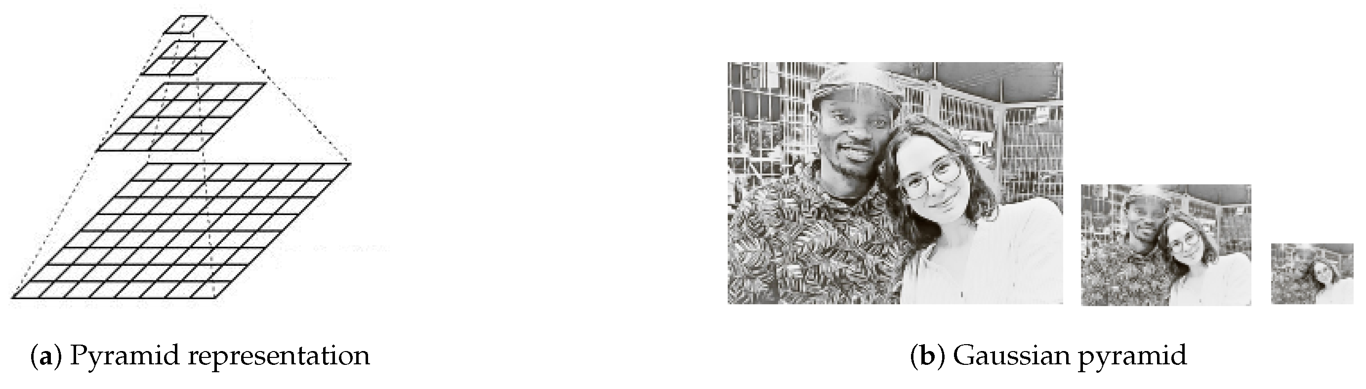
When analyzing an image, it can be helpful to break it down into separate parts so there is no loss of information. The pyramid theory provides ways to decompose images at multiple levels of resolution. It considers a collection of representations of an image in different spatial resolutions, stacked on top of each other, with the highest resolution image at the bottom of the stack and subsequent images appearing over it in descending order of resolution. Such a procedure generates a pyramid-like structure, as shown in
Figure 1a.
The traditional procedure for obtaining a lower-resolution image is to perform low-pass filtering followed by sampling [
21]. In signal processing and computer vision, a pyramid representation is the primary type of multiscale representation for computing image features on different scales. The pyramid is obtained by repeated smoothing and subsampling of an image. Different smoothing kernels have been brought forward for generating the pyramid representation, and the binomial one strikingly shows up as valuable and theoretically well-founded [
22].
Accordingly, for a bidimensional image, the normalized binomial filter may be applied (
,
,
) in most cases twice or even more, along all spatial dimensions. The subsampling of the image by a factor of two follows, which leads to an efficient and compact multilevel representation. There are low-pass and band-pass pyramid types [
23].
To develop filter-based representations by decomposing images into information on multiple scales and extracting features/structures of interest from an image, the Gaussian pyramid (GP), the Laplacian pyramid (LP), and the wavelet pyramid are examples of the most frequently used pyramids. The GP (
Figure 1) consists of a low-pass filter, a reduced density, where subsequent images of the preceding level of the pyramid are weighted down using a Gaussian average or Gaussian blur and scaled down. The original image is defined as the base level. Formally speaking, assuming that
is a two-dimensional image, the GP is recursively defined as presented in (
1).
where
is a weighting function (identical at all levels) termed the generating kernel, which adheres to the following properties: it is separable, symmetric, and each node at level
n contributes the same total weight to nodes at level
. The pyramid name arose because the weighting function nearly approximates a Gaussian function. This pyramid holds local averages on different scales, leveraged for target localization and texture analysis.
Moreover, assuming the GP
, the LP is obtained by computing
, where
represents an upsampled, smoothed version of
of the same dimension. In the literature, LP is used for the analysis, compression, and enhancement of images and graphics applications [
23].
The GP is used in this work for the multiresolution representation of the images right before the feature extraction.
3. Proposed Approach
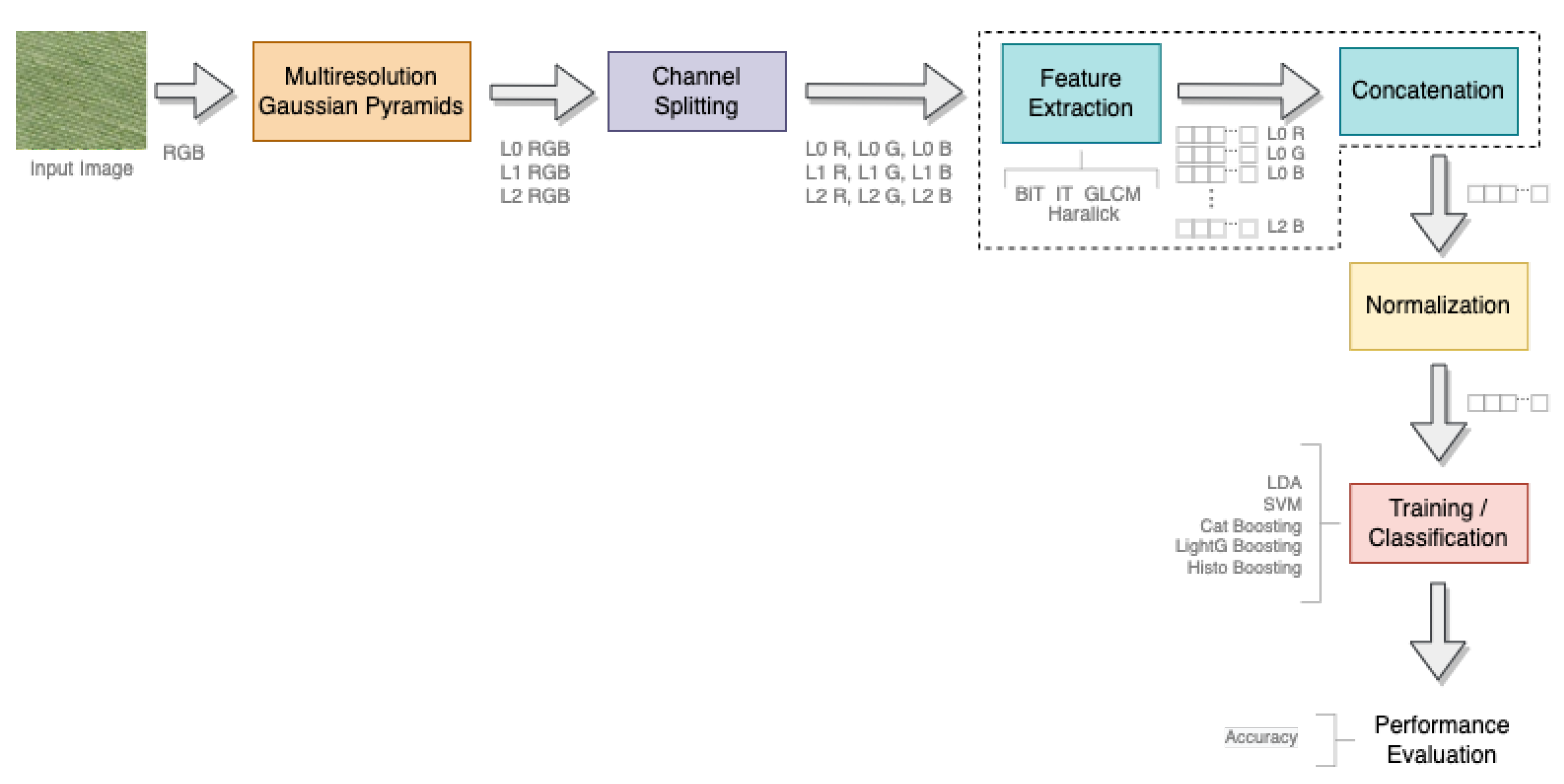
This section describes how the proposed method integrates a multiresolution analysis and multiple texture descriptors for texture classification. To this end, we put forward an architecture structured in five main stages.
Figure 2 shows an overview of the proposed scheme, and Algorithm 1 shows the steps of the first three stages.
Multiresolution representation: In this stage, for an input image, we generate three others corresponding to the levels of the Gaussian pyramid (L0: original image, L1: first level of the pyramid, L2: second level of the pyramid). The purpose is to represent an input image in different resolutions to capture intrinsic details.
Channel splitting: Each channel (R, G, B) is considered a separate input in this phase. The key reason behind the splitting of the channels is to exploit color information. Thus, we represent and characterize an input image in a given resolution by a set of local descriptors generated from the interaction of a pixel with its neighborhood inside a given channel (R, G, or B).
Feature extraction: After the channel-splitting step, the images undergo feature extraction, which looks for intrinsic properties and discriminative characteristics. For each GP level of an image, we extract BiT [
9] (14-dimensional), Shannon entropy and multi-information, i.e., the total information (3-dimensional), Haralick [
4] (13-dimensional), and GLCM [
4] (6-dimensional) descriptors from each channel. Images are then represented by the concatenation of different measurements organized as feature vectors (Algorithm 1). For simplicity, we name the resulting descriptor
three-in-one (TiO). It is worth mentioning that images are converted to a gray scale for GLCM and Haralick measurements to be extracted but remain in color for extracting the bioinspired indices. After feature extraction and before concatenation, the feature vectors have dimensions of 126, 117, 54, and 18 for the BiT, Haralick, GLCM, and Shannon entropy and multi-information descriptors, respectively. Thereby, after concatenation, we have a 315-dimensional feature vector.
Normalization: Because test points simulate real-world data, we split the data into training and test sets and perform a min-max normalization on the training data. Subsequently, we use the same min-max values to normalize the test set.
Training/classification: We have a normalized feature vector comprising the concatenation of features extracted from each resolution and color channel from the previous stage. This texture representation is used to train one monolithic and three ensemble-based models. The linear discriminant analysis (LDA) is used for the monolithic classification model, while ensemble models are created using the histogram-based algorithm for building gradient boosting ensembles of decision trees (HistoB), the light gradient boosting decision trees (LightB), and the CatBoost classifier (
https://catboost.ai/, accessed on 12 January 2023), which is an efficient implementation of the gradient boosting algorithm.
| Algorithm 1: Feature extraction procedure. |
Result: Feature descriptor
1. Read an RGB image file;
2. Generate 3 multiresolution levels with Gaussian pyramids L0, L1, L2;
3. For each level (L0, L1, L2) of Gaussian pyramids;
3.1. Separate the image in channels R, G, B;
3.2. Convert R, G, and B channels to grayscale images (for GLCM and Haralick only);
3.3. Compute bioinspired indices, Shannon entropy, multi-information, Haralick, and GLCM descriptors of R, G, B;
3.4. Concatenate these values into a single vector (315-dimensional);
4. Repeat steps 1 to 4 for all images of the dataset |
It is worth mentioning that the method proposed in this work to improve texture classification concentrates on a multiscale analysis of textural descriptors computed from the surface of 2D images.
Step 3.1 of the algorithm splits the image into different channels, to wit, R, G, and B. The rationale is that there is a difference between processing a 3-channel RGB image and splitting the R, G, and B planes separately in texture analysis. Processing a 3-channel RGB image involves analyzing the image as a single entity, usually a single grayscale image composed of proportions of the R, G, and B channels, i.e., without separating the R, G, and B planes. This is valuable when the patterns or features contained in the image are correlated across multiple planes. For example, if the texture exhibits consistent patterns across the R, G, and B planes, then processing a 3-channel RGB image may be sufficient to capture these patterns. On the other hand, splitting the R, G, and B planes separately allows one to analyze each plane independently and extract features or patterns that are specific to that plane. This is useful when the patterns at different planes are not necessarily correlated or when the patterns at one plane may be obscured by patterns at other planes. By analyzing the R, G, and B planes separately, one can capture the full range of patterns present in the image, even if the patterns are not correlated across the different planes.
Because in texture analysis, the decision between processing the entire 3-channel RGB image or separating the R, G, and B planes rely on the image’s particular properties and the objectives of the analysis, in the experimental sets, we tested both procedures and compared the outcomes to determine which was more suitable; in most cases, splitting R, G, and B planes outperformed the 3-channel RGB image.
As a further factor, in light of the fact that texture forms a nondeterministic system of patterns, we also included features obtained through bioinspired texture descriptors (BiT) in this work. Such descriptors postulate that textural patterns act in a manner that is analogous to ecological patterns, in which populations can self-organize into aggregations that form patterns from the nondeterministic and nonlinear processes that occur inside an ecosystem. In ecology, especially in restoration ecology, summing values to characterize site communities or geographic comparisons of biodiversity therefrom is strongly inefficient if changes in primary resources, such as hydrology, soil, climate, and biology, are ignored. However, considering diversity should unveil changes over time in preserving biodiversity. To this end, splitting the R, G, and B planes separately allows one to analyze each plane independently (as changes in an ecosystem) and extract features or patterns that are specific to that plane (ecosystem in distinct differentiation) to provide feature values that can reflect the background condition and summarize values that describe texture from an image to a great extent under distinct differentiations. This combines the all-inclusive behavior from the R, G, and B planes, instead of solely from the 3-channel RGB image.
4. Experimental Results
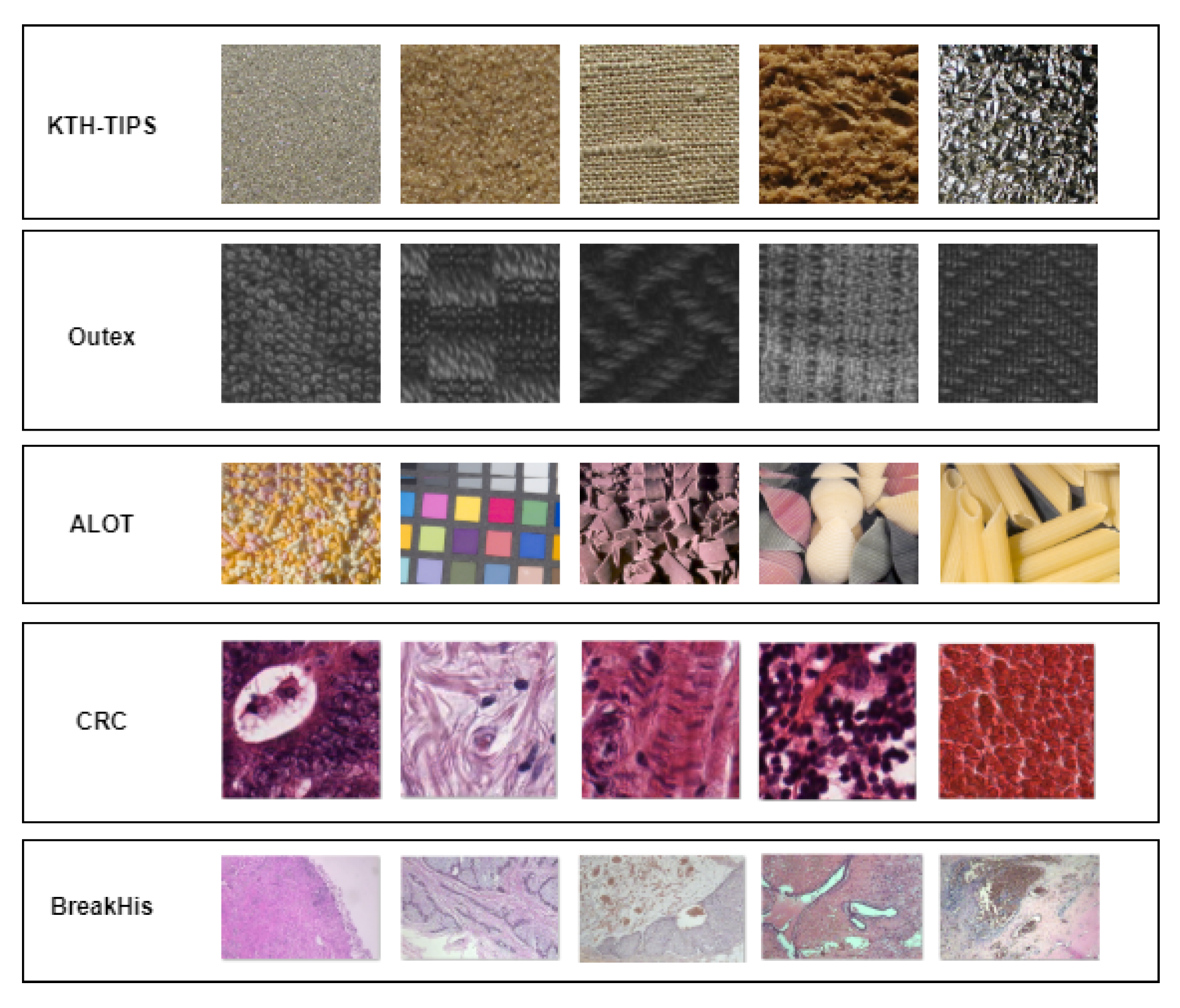
The experimental protocol considered five datasets, three of which are texture image collections, and two are composed of medical images. The KTH-TIPS dataset contains a collection of 810 color texture images of 200 × 200 pixel of resolution. The images were captured at nine scales, under three different illumination directions, and in three different poses, with 81 images per class. Seventy percent of images are used for training, while the remaining 30% are used for testing. The Outex TC 00011-r [
24] has a total of 960 (24 × 20 × 2) images of the illuminant Inca. The training set consists of 480 (24 × 20) images and the test set of 480 (24 × 20) images. The Amsterdam Library of Textures (ALOT) is a color image collection of 250 (classes) rough textures. The authors systematically varied the viewing angle, illumination angle, and illumination color for each material to capture the sensory variation in object recordings. CRC is a dataset of colorectal cancer histopathology images of 5000 × 5000 pixels that were patched into 150 × 150 pixels images and labeled according to eight types of structures. The total number of images is 625 per structure type, resulting in 5000 images. Finally, the BreakHis dataset comprises 9109 microscopic images of breast tumor tissue collected from 82 patients using different magnification factors (40×, 100×, 200×, and 400×). Currently, it contains 2480 benign and 5429 malignant samples (700 × 460 pixels, three-channel RGB, eight-bit depth in each channel, PNG format).
Figure 3 presents samples of images extracted from the KTH-TIPS, Outex, ALOT, CRC, and BreakHis datasets.
We employed two experimentation strategies: a train–test split where 70% of data were reserved for training and hyperparameter tuning, and 30% for testing; (ii) a 10-fold cross-validation. The use of two strategies allowed a better assessment of the performance of the proposed approach and a fair comparison with the state of the art. In the experiments, the full feature vector generated by concatenating all descriptors (TiO) was used for training a monolithic classifier using the LDA algorithm and ensembles using HistoB, LightB, and CatBoost algorithms.
4.1. Experiments with Texture Datasets
There have been numerous important advances in texture classification in the literature during the past few decades. Many of them, however, are new takes on old ideas. Choosing which examples best illustrate the state of the art is difficult. Therefore, we focused on the first ground-breaking initiatives in texture classification. The experimental protocol to assess the proposed approach’s validity included comparisons to important shallow and deep-based methods.
Table 1 and
Table 2 present the results of the proposed method (TiO), BiT, GLCM, and Haralick descriptors on the Outex, KTH-TIPS, and ALOT datasets, using the train–test split and 10-fold cross-validation, respectively. For each dataset, we present the results obtained by combining all the descriptors (TiO) and the results obtained with each descriptor individually. The main purpose was to verify the effectiveness of TiO and the descriptors’ complementary. The proposed method achieved the best average accuracy of 100% on the Outex dataset with the LDA and CatBoost classifiers. On the ALOT dataset, the proposed method achieved an average accuracy of 98.48% with the LDA classifier. Again, TiO outperformed all individual descriptors. Finally, on the KTH-TIPS dataset, the proposed method achieved the best average accuracy of 100% with the LDA classifier. Moreover, TiO outperformed all individual descriptors. Despite the different experimental protocols (train–test split and 10-fold cross-validation), the results were similar for nearly all the classifiers on the respective datasets.
Different works have used the Outex dataset for texture classification. For instance, Mehta and Egiazarian [
25] introduced an approach based on a rotation-invariant LBP, achieving an accuracy of 96.26% with a
k-NN classifier. Du et al. [
26] presented a rotation-invariant, impulse-noise-resistant, and illumination-invariant approach based on a local spiking pattern (LSP). This approach achieved an accuracy of 86.12% with a neural network but was not extended to color textures and required several input parameters. Ataky and Lameiras Koerich [
9] introduced a bioinspired texture descriptor based on biodiversity (species richness and evenness) and taxonomic measures. The latter represented the image as an abstract model of an ecosystem where species’ diversity, richness, and taxonomic distinctiveness measures were extracted. Such a texture descriptor was invariant to rotation, translation, and scale and achieved an accuracy of 99.88% with an SVM.
Table 3 compares our best results with a few works that also used the Outex dataset.
Table 4 presents a few works that also used the ALOT dataset. There was an improvement in the accuracy of nearly 1% and 0.1% compared with shallow and deep methods, respectively. Notwithstanding the difference is not significantly high, it is worth mentioning that the success of CNNs relies on the ability to leverage massive, labeled datasets to learn high-quality representations. Nonetheless, data availability for a few domains may be restricted, so CNNs become restrained from several fields. Moreover, some works evaluated small-scale CNN architectures, such as T-CNN and T-CNN Inception, with 11,900 and 1.5M parameters, respectively. Despite the reduced number of parameters and lower computational cost for training, both still required a large quantity of training data to perform satisfactorily. Even some small architectures of comparable performance, such as MobileNets, EfficientNets, and sparse architectures resulting from pruning, still have many training parameters. For instance, the number of parameters of a MobileNet CNN ranges between 3.5M and 4.2M, while the number of parameters of EfficientNet CNNs range between 5.3M and 66.6M. GoogleNet, ResNet, and VGG CNNs generally need extensive training, and the number of hyperparameters and the computational cost is high.
Likewise, the KTH-TIPS dataset has been used to evaluate texture characterization and classification approaches. Hazgui et al. [
32] introduced an approach that integrated the genetic programming and the fusion of HOG and LBP features, which achieved an accuracy of 91.20% with a
k-NN classifier. Such an approach did not use color information and global features. Nguyen et al. [
33] put forth rotational and noise-invariant statistical binary patterns, which reached an accuracy of 97.73%, lower than the accuracy achieved by the proposed method by about 2.3%. This approach was resolution-sensitive and presented a high computational complexity. Qi et al. [
34] proposed a rotation-invariant multiscale cross-channel LBP (CCLBP) that encoded the cross-channel texture correlation. The CCLBP computed the LBP descriptors in each channel and three scales and computed co-occurrence statistics before concatenating the extracted features. Such an approach achieved an accuracy of 99.01% for three scales with an SVM. Nevertheless, this method was not invariant to scale.
Table 5 shows that the proposed approach outperformed other works that also used the KTH-TIPS.
4.2. Experiments with HI Datasets
Table 6 presents the accuracy achieved by monolithic classifiers and ensemble methods, both trained with the proposed method on the CRC dataset with TiO and BiT, GLCM, and Haralick descriptors, individually. The proposed approach provided its best accuracy of 94.71%, with the HistoB and LightB ensemble models with all feature descriptors. The accuracy difference between TiO and the first best-related work was nearly 2.00%, which corroborated the discriminating ability of our method. Additionally, compared to each descriptor that TiO is made up of, TiO outperformed all of them when employed individually.
Table 7 compares the results achieved by the proposed approach with some state-of-the-art works to assess its effectiveness. The results achieved by TiO on the CRC dataset showed that the proposed approach worked well on images with other structures apart from textures and with no need for data augmentation. Moreover, CNNs need to be trained with a large quantity of labeled data, which may be prohibitive in medical imaging and other related fields.
Table 8 shows the accuracy achieved by monolithic classifiers and ensemble methods trained with all feature descriptors (TiO). For the the BreakHis dataset, the HistoB ensemble model achieved the best accuracy for 40×, 100×, and 400× magnifications, and the LightB ensemble model for a 200× magnification.
Table 9 shows and compares the results achieved by the proposed approach using all feature descriptors with the state of the art for the BreakHis dataset. One can note that the proposed approach achieved a considerable accuracy of 98.64% with all feature descriptors for a 40× magnification, which slightly outperformed the accuracy of both shallow and deep methods. The difference in accuracy between the proposed approach and the second-best method (CNN) was nearly 1% for a 40× magnification. Likewise, the proposed method achieved a considerable accuracy of 97.85%, 98.76%, and 98.22% for 100×, 200×, and 400× magnifications, respectively, which slightly outperformed the second-best method with a difference of 0.9% for 100×, 1.05% for 200×, and 1.0% for 400× magnifications, respectively.
We also conducted additional experiments separately with the BiT, GLCM, and Haralick descriptors. For all the magnifications, TiO outperformed each descriptor with the maximum accuracy difference of 1.25%, 0.48%, 1.01%, 1.5% for 40×, 100×, 200×, and 400× magnifications, respectively. Thus, combining the descriptors mentioned above increased the accuracy by nearly 1%.
5. Discussion
For several reasons, combining multiple feature descriptors can effectively improve the performance and robustness of a texture classification or recognition system. One reason is that different feature descriptors can capture various aspects of the texture, such as frequency, orientation, contrast, and statistical dependencies between pixels. By using multiple feature descriptors, it is possible to capture a complete representation of an image’s texture, which can improve the accuracy of the classification or recognition system. For example, the GLCM descriptor captures statistical dependencies between pairs of pixels in an image, which can help capture texture patterns such as texture boundaries and texture regions. The Haralick descriptor, on the other hand, captures statistical properties of an image, such as contrast and energy, which can help capture texture patterns such as texture density and texture directionality. The BiT descriptor captures the all-inclusive local and global patterns of a textural image. Finally, the Gaussian pyramid captures the spatial frequency content of an image at multiple scales, which can help capture texture patterns such as texture periodicity and texture regularity. Combining these feature descriptors makes it possible to capture a more comprehensive representation of an image’s texture.
As an additional benefit, combining numerous feature descriptors can make a texture classification or recognition system more robust and generalizable. By using multiple feature descriptors, the system can be more resistant to data variations, such as lighting or noise changes. This can be especially important when working with real-world data, where the conditions of the data may be difficult to control. For example, consider a texture classification system designed to recognize the texture of different fabrics. If an automatic system only uses a single feature descriptor, it may be sensitive to lighting variation or background noise, which could affect its performance. However, suppose the system uses multiple feature descriptors. In that case, it may be more robust to these variations, as each feature descriptor may capture different aspects of the texture that are less sensitive to them.
Overall, combining multiple feature descriptors in this work is essential to effectively improve the performance and robustness of a texture classification or recognition system by capturing a more comprehensive representation of an image’s texture and being more resistant to variations in the data.
The proposed approach was assessed with three natural texture image datasets, the Outex, KTH-TIPS, and ALOT datasets, and two HI datasets, CRC, and BreakHis, with 24, 10, 250, 8, and 8 classes, respectively. The experiment protocol employed a train–test split (70/30) and 10-fold cross-validation. For the 70/30 experimental protocol on natural texture images, the results led to the following findings:
The accuracy performance of the BiT, GLCM, and Haralick descriptors on the Outex dataset was not too different, and they all presented an accuracy above 95%. Still, the BiT and Haralick descriptors outperformed the GLCM descriptor with nearly 4% in terms of accuracy using the LDA classifier, the lowest accuracy among all the classifiers. However, since TiO’s performance was roughly equivalent to that of the BiT and Haralick descriptors for the Outex dataset, such a combination was not necessary to this extent.
Along the same line, the accuracy performance of the BiT and Haralick descriptors on the KTH-TIPS dataset was similar, regardless of the classifier. The GLCM descriptor, nonetheless, showed a difference of about 11% (with its lowest accuracy) and 7% (with its highest accuracy) compared with the BiT and Haralick descriptors. However, the difference was insignificant when comparing the best descriptor, BiT, with TiO. Therefore, for the KTH-TIPS dataset, such a combination brought a slight improvement.
Unlike the Outex and KTH-TIPS datasets, the presented concatenation played a significant role in the classification performance of the ALOT dataset. First, the best performance of all the datasets was obtained with the LDA classifier. The highest accuracy performance with TiO was 98.48%, outperforming the BiT, GLCM, and Haralick descriptors by nearly 20%, 32%, and 14%, respectively. The lowest difference, 14%, was still a significant improvement. Such a classification performance is promising as it is above several state-of-the-art deep methods on the ALOT dataset. The ALOT dataset is challenging due to different variations in images regarding viewing angle, illumination angle, and color.
Furthermore, the combination of BiT, GLCM, and Haralick descriptors provided a state-of-the-art classification performance on HIs.
Notwithstanding, one states that an effective feature selection may be necessary to derive subsets of relevant features from each descriptor such that each dataset can be characterized to the maximum extent with as minimum a feature dimension as possible. Finally, it is worth mentioning that the experimental protocol with a train–test split and 10-fold cross-validation provided similar results.
6. Conclusions
This research provided a critical study regarding image analysis and manipulation over a spectrum of spatial scales and the complementarity of feature descriptors for texture classification. We stated that employing each descriptor separately may overlook relevant textural information, reducing the classification performance. Moreover, we exploited the pyramid’s multiresolution representation as a useful data structure for analyzing and capturing intrinsic details from texture over a spectrum of spatial scales. To produce a feature vector from an image, we combined several descriptors that were proven to be discriminating for the classification, namely, the BiT, information-theoretic measures, GLCM, and Haralick descriptors, to extract gray-level and color features at different resolutions. Such a combination aimed to bring features that characterized the texture to the maximum extent and with some advantages such as rotation-, permutation-, scale-invariance, reduced noise sensitivity, and a generic and high generalization ability, as it provided an effective performance for real-world datasets.
The proposed approach outperformed a few state-of-the-art shallow and deep methods. Moreover, the descriptors employed herein were proven complementary as their combination resulted in a better performance than using each separately. However, some features may be redundant after the concatenation into a single feature vector, given the different resolutions, channels, and descriptors. That may cause a downfall in the classification performance. Furthermore, such a concatenation may also lead to the Hughes phenomenon, which explains why we did not include other descriptors such as LBP, HOG, etc. However, we will consider including other descriptors in our future studies. Finally, to circumvent the possible feature redundancy and cope with the increase in dimensionality, we will investigate the impact of incorporating a decision-making multiobjective feature selection.

 ,
, 


