Article

Predicting Temperature and Humidity in Roadway with Water Trickling Using Principal Component Analysis-Long Short-Term Memory-Genetic Algorithm Method

1
Key Laboratory of Deep Coal Resource Mining (CUMT), Ministry of Education of China, School of Mines, China University of Mining and Technology, Xuzhou 221116, China
2
College of Safety and Emergency Management Engineering, Taiyuan University of Technology, Taiyuan 030024, China
*
Authors to whom correspondence should be addressed.
Appl. Sci. 2023, 13(24), 13343; https://doi.org/10.3390/app132413343
Submission received: 23 October 2023 / Revised: 11 December 2023 / Accepted: 13 December 2023 / Published: 18 December 2023
(This article belongs to the Topic Complex Rock Mechanics Problems and Solutions)

Abstract

:
The heat dissipated from high geo-temperature underground surrounding rocks is the main heat source of working faces, while thermal water upwelling and trickling into the roadway will notably deteriorate the mine’s climate and thermal comfort. Predicting airflow temperature and relative humidity (RH) is conductive to intelligent control of air conditioning cooling and ventilation regulation. To accommodate this issue, an intelligent technique was proposed, integrating a genetic algorithm (GA) and long short-term memory (LSTM) based on rock temperature, inlet air temperature, water temperature, water flow rate, RH, and ventilation time. A total of 21 input features including over 200 pieces of data were collected from an independently developed modeling roadway to construct a dataset. Principal component analysis (PCA) was conducted to reduce features, and GA was used to tune the LSTM and PCA-LSTM architectures for best performance. The following research results were yielded. The proposed PCA-LSTM-GA model is more reliable and efficient than the single LSTM model or hybrid LSTM-GA model in predicting the air temperature T f o u t and humidity R H o u t at the end of the water trickling roadway. The importance scores (ISs) indicate that T f o u t is mainly influenced by the surrounding rock temperature (IS 0.661) and the inlet air temperature (IS 0.264). While R H o u t is primarily influenced by the rock temperature in the water trickling section (IS 0.577), the inlet air temperature (IS 0.187), and the trickling water temperature and flow rate (total IS 0.136), and it has an evident time effect. In addition, we developed relevant equipment and provided engineering practice methods to use the machine learning model. The proposed model, which can predict the mine microclimate, serves to facilitate coal and geothermal resource co-mining as well as thermal hazard control.

1. Introduction

Unlike hazards of gas, fire, water, and roof, thermal hazards, which are considered non-fatal and tolerable for underground workers, have not been focused on for a long time. However, this issue has become an unavoidable global issue with deep-mining and occupational health system improvement [1,2,3]. There are up to 47 deep mines with a depth over one kilometer in China, such as Suncun Coal Mine (1500 m) and Jiahe Coal Mine (1200 m), all of which have reached the criteria for Grade III thermal hazard (airflow temperature ≥ 32 °C) [4,5,6]. Low-level thermal hazards can be alleviated by properly increasing the airflow speed. However, mines with severe thermal hazards must be equipped with air-conditioning cooling systems (e.g., air cooling, water cooling [7], and HEMS cooling [8]). Mine intelligent ventilation (MIV) is an important safeguard for intelligent mining, and its goal for hot mines is to achieve airflow and cooling regulation according to the needs for mine climate condition improvement and disaster relief [9]. To accommodate this goal, firstly, the layout of sensors should be optimized, including air velocity and pressure sensors, airflow temperature and humidity sensors, and fan operation monitoring sensors, to conduct data intelligence and processing. In particular, the evaluation of the thermal comfort based on the underground microclimate is of necessity. Secondly, a real-time network solution should be provided to accurately identify abnormality and give prewarning (e.g., gas, dust, heat). It will take a certain time from the above visualization to regulation, which is a gray time period with hidden safety trouble, so it can be seen that such regulation has some lag. For this reason, distributing air volume and cold capacity according to the needs predicted in advance is the key link of intelligent decision making. Finally, coordinated control of equipment is realized to carry out automatic regulation of the flow resistance and the working conditions of air-conditioning and mine ventilators. Therefore, predicting airflow humidity and temperature in the roadway conduces to intelligent control of air-conditioning cooling and ventilating regulation, and finally serves to facilitate coal and geothermal resource co-mining as well as thermal hazard control under the background of deep mining and MIV.
In respect of heat exchange, the airflow temperature rise is mainly from the heat dissipated by the surrounding rocks [10], especially when the airflow is transported through a long distance from the pit bottom to the working face (Figure 1). The heat is exchanged between airflow and surrounding rock unsteadily, in a complex manner [11], and its theoretical calculation is based on the unstable heat exchange coefficient K τ derived from the concept of the temperature regulation sphere. Many scholars have established methods to find the solution of K τ , including the accurate solution method [12,13], the Laplace transform method [14,15], the variable separation method [16], and the numerical solution method [17,18], but the solution finding processes are relatively complex. Because of the non-linearity of the differential equations of heat conduction, these methods have poor usability. For this reason, some scholars have proposed empirical equations for calculation of the airflow temperature based on the statistics and fuzzy mathematics, etc. [19,20]. However, each of these equations is typically a multivariate function, so when the application scope is beyond the statistical scope, the error will be relatively large. In recent years, the numerical calculation models (e.g., FEM and FVM) for a single line of surrounding rock–airflow heat transfer have been included in the scholars’ discussion scope [21,22,23]; nevertheless, since the relationships between the air temperature and numerous influencing factors (e.g., wall roughness, thermal physical parameters of rock, and moisture content of airflow) are highly nonlinear, scholars find it extremely hard to figure out parameters in these models. In addition, the models are rarely applied to whole ventilation networks on engineering sites as a result of missing parameters, deficient validation, and insufficient an description of the heat and mass transfer mechanisms. In fact, the heat released by thermal water upwelling from rock fractures or by high-temperature surrounding rocks coming into contact with the thermal water is non-negligible in the calculation of heat sources in a mine [24,25,26]. The mass transfer in a roadway with humid air is less focused on. Liu [27] and Gao [28] introduced the “wall wetness degree” to correct K τ , and Li [29] constructed an airflow heat exchange coefficient correction function for a roadway with water trickling, using an airflow rate weighted distance to describe the change law of relative humidity of the airflow in an actual mine network area. As described above, research efforts on the prediction of underground airflow humidity and temperature are insufficient, for which the reasons are as follows: (1) the factors influencing temperature or humidity are numerous; (2) it is hard to master the coupling law between heat exchange and moisture exchange; and (3) the usability is insufficient, and the prediction accuracy may be high for a single or short-distance line but the models cannot be popularized to the whole network or long-distance lines.
Numerical simulation is an effective method for scholars to study the change of temperature and humidity in a roadway. Based on numerical simulation, Xu et al. [30] and Li et al. [31] explored the flow and heat transfer law of thermal fluid during geothermal mining in rock strata. Their exploration results revealed that the temperature of the surrounding rock of a roadway decreases gradually, and the temperature rise of the air flow in a roadway is reduced during the process of water injection in rock strata. Zhang [32] investigated the effect of the seepage of cryogenic fluid on the surrounding rock temperature, and found that the fissure seepage can control the distribution of surrounding rock temperature in a high-temperature roadway. Nevertheless, the modeling process in numerical simulation always deviates from the actual situation on the spot, leading to unsatisfactory results. Moreover, the numerical simulation cannot be updated in real time, thus failing to predict the change of tunnel climate effectively. Machine learning (ML) refers to learning algorithms adopted for searching the optimum prediction model with the aid of big data [33,34,35]. In recent years, ML has been widely employed in mining engineering applications, such as gas emission [36], mine water inflow [37], shield pressure monitoring [38], and air quality and pollutant monitoring [39], to adapt to such characteristics of various problems under the combination of multiple factors such as a large number of data, and strong non-linearity [40,41,42]. In terms of predicting the underground microclimate, Li [43] established an actual mathematical model based on the thermal conductivity inside tunnels, and compiled a corresponding program for prediction, which has been applied to practical projects. However, the influence of cryogenic fluid on temperature was omitted in this mathematical model. Currently, problems remain in utilizing ML to predict the underground microclimate. In particular, ML applications are exiguous, and the temporal correlation among mining data is ignored when predicting temperature changes for a lack of establishment and administration of a mine thermal environment database. In addition, the in situ observation and artificial acquisition of data are arduous. For example, Marc Bascompta [44] acquired the data of such variables as dry/wet temperature and airflow, at seven control points continuously for 3 years, and this process consumed excessive time and funds. Fortunately, similarity simulation experiments can remarkably shorten the time. In this study, a physical similarity simulation device was developed. Unlike the devices designed by Wang et al. [45], Zhang et al. [46], and Zhu et al. [19], this device was specially equipped with a water trickling system that can adjust the trickling water flow rate and temperature and collect the humidity and temperature data of airflow after it passes through the water trickling section of roadway. Meanwhile, the temperature changes in surrounding rock at various depths can be observed through it in real time. Hence, the problem of difficult data collection was solved. Furthermore, to explore the temporal correlation among data, LSTM was applied to the prediction of the underground microclimate, thus ensuring the accuracy of the prediction results.
In this study, a novel hybrid model PCA-LSTM-GA based on the advantages of individual models was developed for more efficiently predicting air humidity and temperature in an underground roadway with water trickling. Firstly, 21 input features and over 200 pieces of data were acquired with the independently developed modeling roadway. Then, training and testing were conducted using the ML model. The predictive capability of the model was validated with the coefficient of determination ( R 2 ) and mean square error (MSE). Finally, analysis of variable importance was carried out to guide engineering practice. The other highlight of the present study is that the proposed data acquisition method can be used in engineering practice, and relevant equipment has been developed, greatly promoting the proposition.

2. Dataset Preparation

2.1. Research Area Description
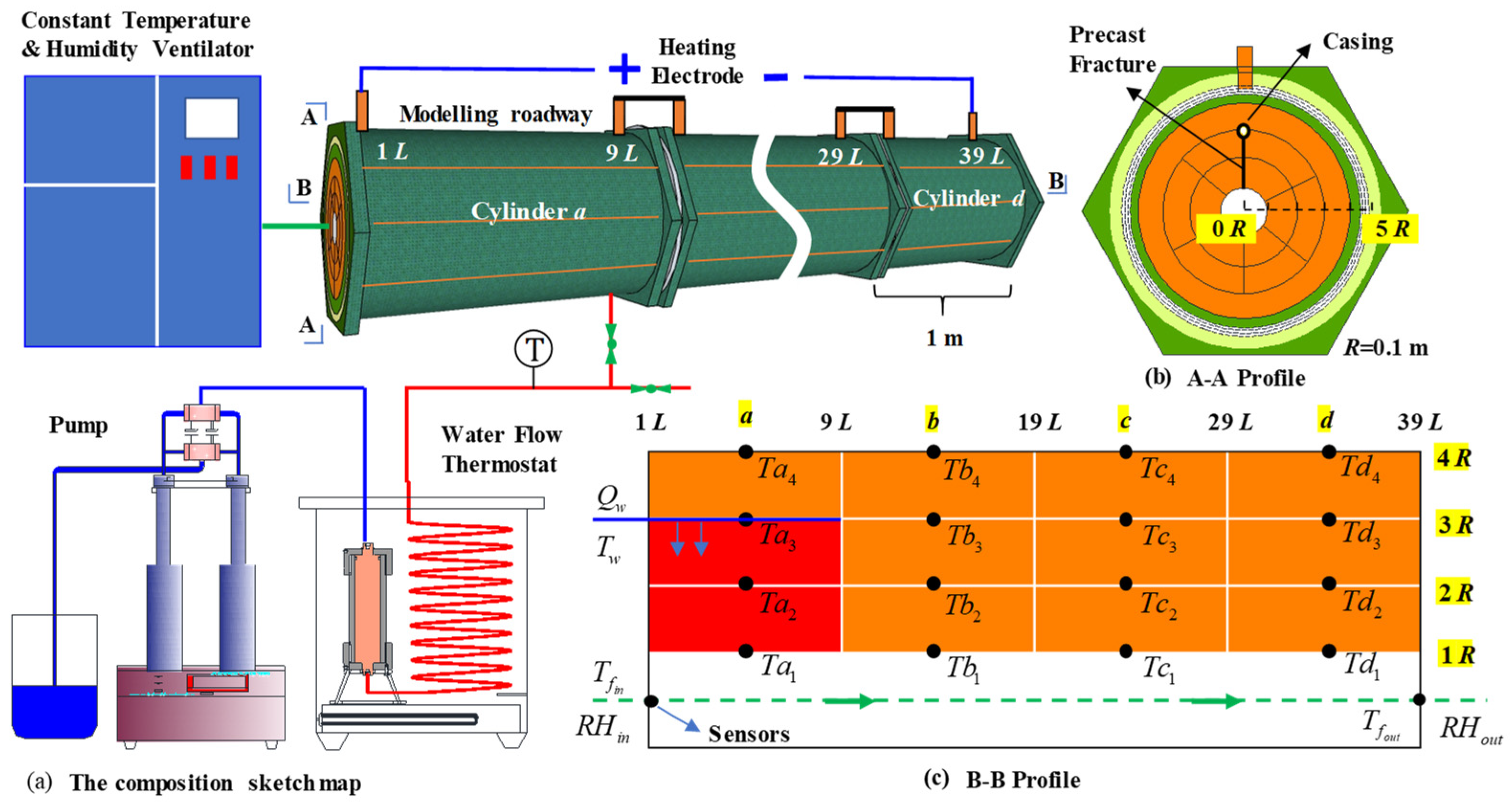
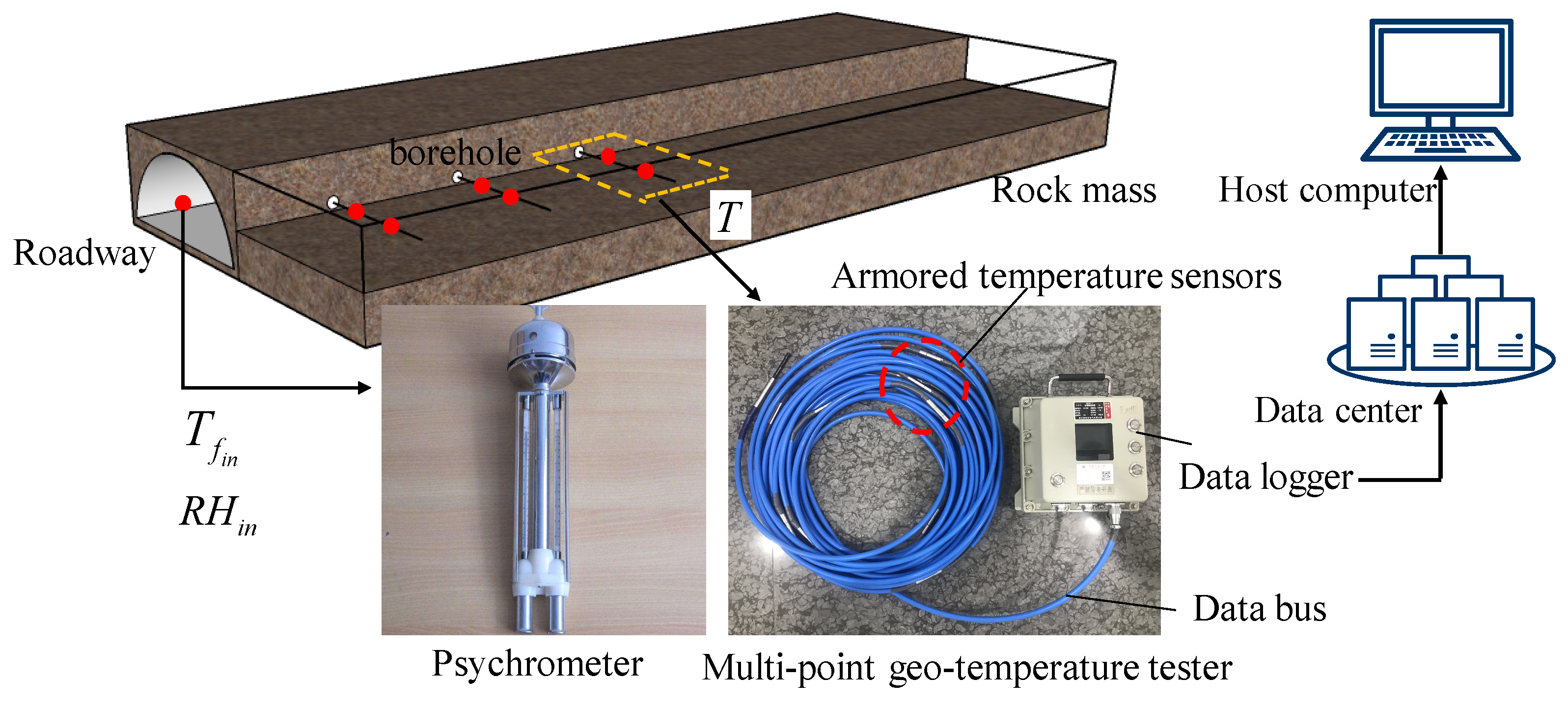
Located in Xuzhou, China, Sanhejian Coal Mine is a typical mine plagued by thermal hazards. The heat mainly comes from high geo-temperature (HGT) surrounding rock where the temperature at −700 m level can reach 37–40 °C (Figure 1b), and 42–49.4 °C at −980 m level. The high temperature is mainly caused by regional geothermal accumulation and heat transfer condition changes in the shallow crust, specifically speaking, including the high terrestrial heat flow, high thermal resistance cover, and basement rock fluctuations. In addition, thermal water upwelling and trickling (TWUT) also heats and humidifies the air and notably deteriorates the mine climate. The Shunshidian Fault in the northeast of Sanhejian mining area is cut through by the neotectonic faults. Consequently, the Ordovician limestone aquifer remains able to laterally conduct water (Figure 1c). The water head (~980 m) between the suboutcrop area and trickling area provides flow dynamic to make the heated underground water deeply circulate, upwell along the fracture and fault, and ultimately trickle into the roadway.
The microclimate parameters along the ventilation route of the A-I working face recorded in March 2018 are given in Figure 2a. The results show that Sanhejian Coal Mine is a typical high-humidity and high-temperature mine (Figure 2). The airflow temperature rose from 27.4 °C at the pithead to 27.4 °C at the working face, and the relative humidities (RH) at all measurement points exceed 85%. The enthalpy of moist air i and the enthalpy of water vapor i v both surged after the airflow passed through the YWUT zone, and the i v / i value at the end of the route was greater than 70%. Such a result suggests that a great proportion of heat came from the latent heat exchange of airflow.

2.2. Apparatus

In this study, an experimental apparatus for heat and mass transfer (EAHMT) was designed and developed in the hope of obtaining microclimate parameters (humidity, temperature, airflow speed, etc.) of the HGT and TWUT mine. The composition sketch map of EAHMT is illustrated in Figure 3. The modeling cylinders poured with similar simulation materials were electrically heated from room temperature to a constant virgin rock temperature 60 °C, and the direct current (0–1000 A) converted by a rectifier flowed through the heating electrode and alloy heating network (at 5 R), which connected the different cylinders (a–d). To simplify the model, the surrounding rock fractures in Figure 1c were made equivalent to a fracture zone. Therefore, in pouring of materials in the TWUT section (1–9 L), a 2 mm fracture face towards the roadway was precast in the scope of 1–3 R along the radial direction, and a designed casing was pre-embedded at 3 R in the axial direction (Figure 3b). The casing was a coaxial double-layer steel tube, of which inner and outer sleeves were grooved upwards and downwards, respectively. First, the surfactant-containing water was filled into the inner sleeve after the surface tension was overcome. Subsequently, the water evenly flowed into the outer sleeve, and finally flowed into the roadway along the fractures in a relatively even manner. The water temperature and flow rate could be controlled by the thermostat and pump.

2.3. Dataset Used

The values of input and output variables of the machine learning model were acquired with the EAHMT. The arrangement of sensors is shown in Figure 3c. The experiment of each group had three stages: in Stage 1 (~24 h), the surrounding rocks were heated to a predetermined temperature, to simulate the virgin rock temperature before roadway excavation; in Stage 2 (~2 h), ventilation was maintained, to cause thermal disturbance in surrounding rocks until heat balance was reached between the surrounding rocks and airflow; and in Stage 3 (~3 h): supply of thermal water was maintained until heat and humidity balance was reached among the surrounding rocks, airflow, and fracture water. The dataset used in this study was from Stage 3, in which the thermal water trickling caused the change of the airflow microclimate to be so complex that it was difficult to predict with conventional theoretical models.
The output variables of the model were the airflow humidity R H o u t and temperature T f o u t at the end of the roadway with water trickling. To better predict the output values, the input variables included 21 features, including rock temperature T (16 measuring points), trickling water temperature T w , trickling water flow rate Q w , inlet airflow humidity R H i n , inlet airflow temperature T f i n , and ventilation time τ .
T and τ : The temperature of the rock not undergoing engineering disturbance in strata is called virgin rock temperature T 0 . Figure 4 shows the temperature variation of surrounding rock in cylinder a in Stage 2. After roadway excavation, the roadway wall temperature T a 1 fell sharply as ventilation started. Temperature difference occurred in the surrounding rocks, so the heat conduction process occurred accordingly, and the thermal disturbance scope in the surrounding rocks was enlarged gradually over time τ . Finally, the heat flux in surrounding rocks tended to be consistent, indicating re-balance of temperature field of surrounding rocks after disturbance. Therefore, during heat dissipation from surrounding rocks to the airflow, the temperatures at 16 measuring points for surrounding rocks in Figure 3c exhibited different variation characteristics with the ventilation time τ , in other words, this feature also reflected the time of ventilation and that of heat dissipation from surrounding rocks.
T f i n and R H i n : The airflow exhibits heat and humidity accumulation effects during long-distance transport. Hence, the airflow humidity and temperature at the inlet are of important significance for prediction of airflow humidity and temperature at the end. At the same water vapor content, RH is related to temperature. The higher the temperature is, the greater the saturated humidity ratio in the air will be, which means that the stronger the hygroscopicity of the air will be.
T w and Q w : Different upwelling water temperatures and flow rates directly influence the humidity and temperature of airflow passing through the water upwelling section. For example, at high upwelling water temperature, the humidity ratio variation rates at various points after the water upwelling section make it difficult to achieve synchronism at the early stage. In Sanhejian Coal Mine, the water upwelling flow rate is normally not more than 3 m 3 / h within 16 m, and it should not be more than 250 mL/min in the similarity ratio conversion experiment. The Ordovician limestone water temperature in Sanhejian Coal Mine is 50 °C, the maximum upwelling water temperature in China’s coal mines is 60–70 °C (for example, the temperature is 65 °C in Pingdingshan No. 8 Mine), and the upwelling water temperature in some metal mines can reach 70–80 °C (for example, the upwelling water temperature is 73.5 °C in Jiudian Gold Mine). Therefore, the upwelling water flow rate in the experiment was set to 50, 100, and 200 mL/min, and the upwelling water temperature was set to 40 °C, 60 °C, and 80 °C.
The preliminary analysis of data regarding feature parameters is listed in Table 1.

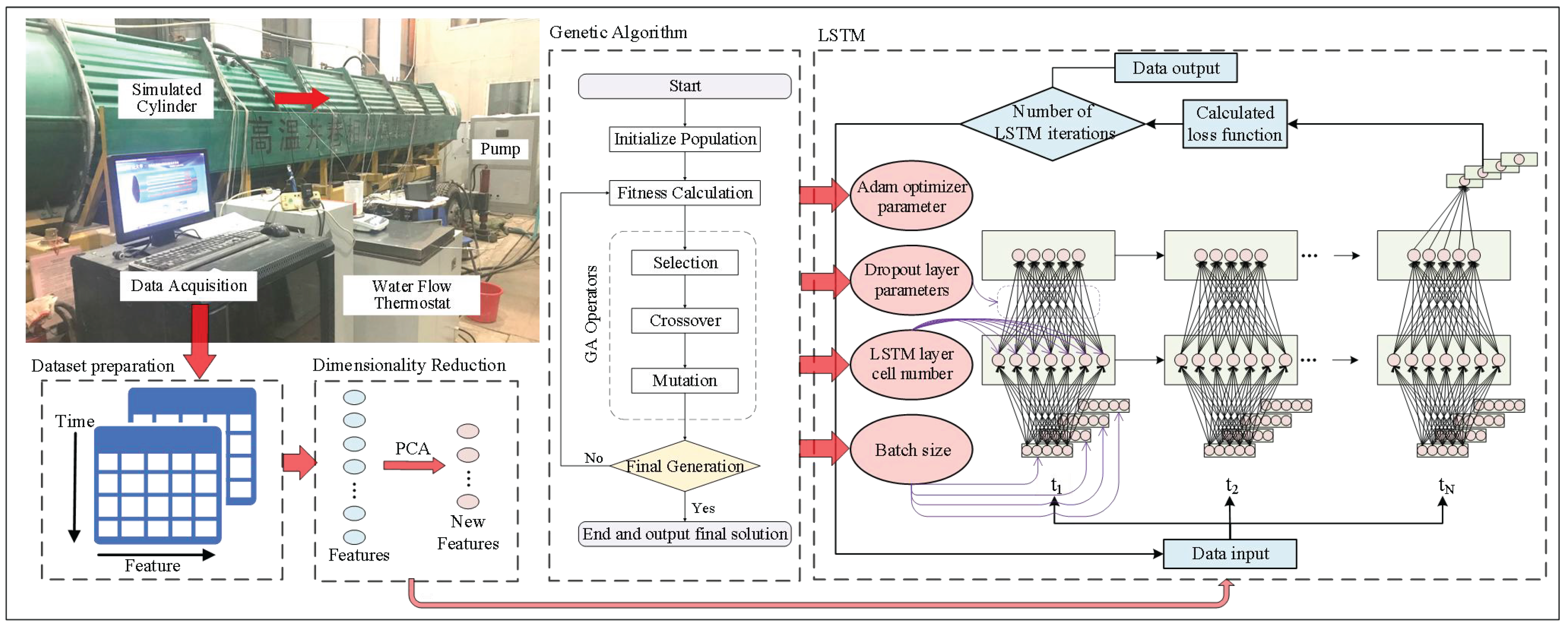
3. Machine Learning Modeling

3.1. Fundamental Theory of PCA, LSTM, and GA

3.1.1. PCA

Principal component analysis (PCA), as a kind of unsupervised feature reduction method [47], normalizes the original data first, and then extracts important components with non-repetitive correlations from the processed data, to effectively decrease the influences of interfering data, and thus to achieve the purpose of raising the accuracy of recognition (regression or clustering) and lessening the feature dimensions of data [48,49]. The specific procedure is introduced bellow:
(1)
The original data are normalized for the purpose of eliminating the impact of dimensions on the calculation results. On this basis, the original matrix X is established.
(2)
The covariance matrix P can be determined based on Equation (1), and then can eigenvalues λ i and eigenvectors α i be obtained.
P = 1 S 1 ( X * ) T X *
where S is the number of samples.
(3)
The number of principal components can be calculated by Equation (2):
a = min { k i = 1 k λ i / i = 1 n λ i δ }
where δ is the threshold value of the cumulative contribution rate, normally set at 85%; and i = 1 k λ i / i = 1 n λ i is the cumulative contribution rate of principal components of the first k eigenvalues (k < n).
(4)
The original matrix can be dimension reduced by combining the covariance matrix P and the number of principal components a .

3.1.2. LSTM Networks

Long short-term memory (LSTM) is a promoted recurrent neural network (RNN)-based network structure, and its particularity lies in the fact that the nerve cells in the RNN are replaced with memory blocks [50,51]. Each memory block includes one or more memory cells and three non-linear summation units, and the whole neuron is controlled by the gate. Therefore, the LSTM not only is pretty proficient in handling issues highly related to time series, but also resolves gradient dispersion of the RNN occurring during training [52].
Figure 5 shows the internal structure of a nerve cell of the LSTM at three consecutive time points. It can be seen that the input part (marked in red) includes the current input x t , the memory from the last LSTM unit C t 1 and the output of the last LSTM unit h t 1 , and the output part (marked in blue) includes the current output h t , the next hidden state h t , and the next cell state C t . The keys of the LSTM are the cell state and the gates (including the forget gate f t , the input gate i t , and the output gate O t ). The cell state resembles a conveyor belt to some extent. The structures of the gates can remove or add information to the cell state, and thus describe the quantity of information contained in the current network. First, the data pass through the forget gate for information filtering, during which xt (input at time t) and ht−1 (output of the hidden layer at the previous moment) are substituted to the σ function to generate values within the range of 0–1. Values 0 and 1, respectively, indicate that none or all historical data are retained. Next, information that can be used for processor state updating is determined and stored through the input gate it. Finally, the output gate Ot determines the amount of information to be output based on the new cell state. Ot signifies the degree of choice between the current information and the input information, and ht represents the predicted output. The operating principle of the cell follows Equations (3)–(8).
f t = σ W f h t 1 , x t + b f
i t = σ W i h t 1 , x t + b i
C ˜ t = tanh W C h t 1 , x t + b C
C t = f t C t 1 + i t C ˜ t
O t = σ W O h t 1 , x t + b O
h t = O t tanh ( C t )
where C denotes the cell state, C ~ denotes the storage information of new data, t a n h and σ are both activation functions, W is the weight matrices connecting the hidden state h t 1 and the input sequence x t , and b are the bias vectors.

3.1.3. GA

In this study, MSE was taken as the objective function for calculating the values of the hyperparameters in the LSTM, and the genetic algorithm (GA) was applied to LSTM optimization. GA was inspired by gene recombination, gene crossover, and gene mutation in nature [53,54,55]. Its principle is illustrated in Figure 6. This algorithm mainly involves binary encoding and decoding of the population, calculation of genetic operators, and calculation of individual fitnesses [56,57]. The specific calculation procedure is as follows.
(1)
Population initialization: binary encoding is utilized to convert feasible solutions in the problem space into genotype string structures in the genetic space, and the initial population is generated.
(2)
Individual evaluation: the fitness function values of individuals in the initial population are calculated.
(3)
Genetic operator calculation: new individuals are generated through three paths, namely selection operator, crossover operator, and mutation operator.
(4)
Whether the iteration conditions are met is identified. If not, Step 2 is conducted; otherwise, the optimal individual is decoded, and the optimal solution is output.
Figure 6. Framework of the PCA-LSTM-GA model.
Applsci 13 13343 g006

3.2. Modeling and Hyperparameter Tuning

The airflow humidity and temperature data at different positions have close spatiotemporal relationships and have unstable gradient variation. To accommodate this issue and to make full use of the spatiotemporal properties implied by the data, a prediction model for airflow humidity and temperature data was constructed here based on the LSTM model for the time sequence problem. Since the input features of this model were as many as 21, there might be problems of parameter redundancy and lowered training speed occurring. Furthermore, artificial selection of model parameters will typically not make the model have an optimal performance. In this paper, to make the model have the optimal effect, dimension reduction was conducted for the input parameters of the model using the PCA algorithm, and intelligent optimization was carried out for the model after dimension reduction using the GA, to select the optimal parameter values for the model, and thus to construct a prediction model for humidity and temperature at the end of the roadway based on PCA-LSTM-GA.
Since how the model performs is affected by both the neural network structure and the model parameters, the number of units in the LSTM layer, dropout layer parameter, batch size, and optimizer learning rate were selected as optimization objects for GA (Figure 6). An LSTM network model was established based on the values taken for the initial hyperparameters, and it was trained with the training data. Prediction was carried out with the test data put into the trained model, and optimization was conducted with the error generated by the model in the test dataset as the optimization target until the termination condition was met. Finally, an LSTM network model was constructed with optimum values of the hyperparameters.
In this study, the PCA-LSTM network model mainly contained four layers, namely the input layer, LSTM layer, dropout layer, and output layer. MSE was used as the loss function, and Adam was selected as the optimization algorithm. The dropout layer parameter, batch size, and optimizer learning rate were set as hyperparameters of the LSTM network model. The value ranges for optimization of hyperparameters were set as follows: [10, 100] for the number of units in the LSTM layer, [0.1, 0.3] for the dropout layer parameter, [5, 25] for the batch size, and [0.0001, 0.01] for the Adam optimizer learning rate.
Comparatively, the LSTM model comprised the input layer, LSTM layer (with number of units of 60), dropout layer (with parameter of 0.1), and output layer, and the Adam optimizer learning rate was 0.001. The loss function used was also the MSE.
Both the experimental models were constructed with the Keras. An introduction of the algorithm flow is as follows:
Step 1 (dataset preprocessing): first, the original dataset is divided into the training set and the testing set. Next, the cumulative contribution rates of the principal components are determined. Subsequently, the original experimental data are dimension reduced (from the initial 21 dimensions to 5 dimensions) through PCA, and the data after dimension reduction are taken as input for the neural network model.
Step 2 (model construction): first, an LSTM neural network model is constructed. Then, GA is utilized to calculate the batch size, learning rate, and dropout layer parameters of the constructed model with MSE as the objective function.
Step 3 (model generalization ability verification): the prediction performance of the model on the testing set is validated by taking R 2 and MSE as evaluation indices.

3.3. Assessment

The assessment included two parts: one was to assess the energy variation of the airflow caused by the upwelling water temperature and flow rate, and the other was to assess the predictive capability of the models.
Humidity and heat exchange occurs between airflow and thermal water during water passing through, and the power driving the heat and humidity exchange is an enthalpy difference [58]. The latent heat variation can be characterized with the enthalpy difference of the water vapor, and the sensible heat variation is characterized with the enthalpy difference of the dry air. The total enthalpy difference of the airflow reflects the airflow energy change and also serves as the basis for calculation of the coldness needed for roadway cooling, and it is calculated with Equations (9)–(12):
Δ i = Δ i 39 L Δ i 1 L = ( i 39 L F i 39 L S ) ( i 1 L F i 1 L S )
i = 1.0045 t d + d ( 2501 + 1.85 t d )
d = 0.622 φ f 1 / ( P 1 φ f 1 )
f 1 = 0.6099 exp 17.27 t d / ( 237.3 + t d )
where Δ i is the enthalpy difference, k J / k g ; i 39 L F and i 39 L S are the enthalpies at a position 39L at the beginning and end of water passing through, respectively, k J / k g ; i 1 L F and i 1 L S have a similar meaning to the above; 1.0045 t d represents the enthalpy of 1 kg of dry air, k J / k g ; d denotes the humidity ratio in air, k g / k g ; 2501 is the latent heat of vaporization of water vapor, k J / k g ; 1.85 is the mean specific heat at constant pressure of water vapor at normal temperature, k J / ( k g · K ) ; t d is the dry bulb temperature, °C; φ is the relative humidity of air, % ; P 1 is the atmospheric pressure, K P a ; and f 1 is the saturated vapor pressure of air at t d , k P a .
Regarding the generalization ability of the constructed model, MSE and R 2 , two parameters extensively used for reflecting the generalization ability of models from different aspects [35,59,60], were selected as evaluation indices. Their expressions are given as:
MSE = 1 m i = 1 m ( y ( i ) y ^ ( i ) ) 2
R 2 = 1 i = 1 m ( y ^ ( i ) y ( i ) ) 2 i = 1 m ( y ¯ y ( i ) ) 2
where m is the number of samples; y ( i ) is the actual value of sample i; y ^ ( i ) is the predicted value of sample i; and y ¯ is the average value of the samples.

4. Results and Discussion

4.1. Total Enthalpy Difference Variation in Roadway with Water Trickling

Figure 7 shows the variation curves of total enthalpy difference Δ i of airflow in a roadway at different upwelling water temperatures and flow rates. The increase in upwelling water temperature results in simultaneous increase in sensible heat and latent heat of airflow, as shown in Figure 7a. At the same upwelling water flow rate (100 mL/min), the Δ i of humid air exhibits a non-linear ascending trend and that of dry air rises slightly with the increase in upwelling water temperature. The increase in upwelling water flow rate rarely influences the sensible heat of airflow. Instead, it mainly leads to the increase in latent heat of airflow, as shown in Figure 7b. At the same temperature (60 °C), the Δ i of humid air (including water vapor) exhibits a linear ascending trend and that of dry air fluctuates with the increase in upwelling water flow rate.

4.2. Hyperparameter Tuning

It is necessary to set the parameters of GA before the LSTM is performed. After plentiful tests, the relevant parameters were finally determined as follows: maximum iteration number 100; chromosome number (for each generation) 20; algorithm chromosome selection; crossover probability 0.20; and mutation probability 0.02.
The performance of the deep-learning network on the testing set was used as the optimization target in the intelligent hyperparameter optimization based on GA, and the specific reflection was that the MSE value of the network on the testing set was used as the fitness value of the GA. In the GA, one chromosome was used to represent a group of hyperparameters. The gene sequence was updated through chromosome evolution, to minimize the fitness value. The optimal hyperparameter values were selected after optimization of the GA. Finally, the LSTM model with the optimal hyperparameter values was validated experimentally.
As above mentioned, the hyperparameters of the LSTM network were tuned by the GA. As shown in Figure 8a,b, the effectiveness of the hyperparameters was tuned by tracking the MSE value obtained from every iteration. The MSE values of both the prediction model for temperature at the end of the roadway and that for humidity at the end of the roadway decrease significantly in the initial stage of iteration, which is indicative of effectiveness of the GA in tuning the hyperparameters. It is worth mentioning that both the humidity and temperature models processed through dimension reduction by the PCA have a better fitness performance in the initial stage of parameter optimization than those not processed through dimension reduction by the PCA, which can also demonstrate to a certain extent that the dimension reduction by the PCA is of positive significance for improvement of model performance.

4.3. Predictive Capability of the Models
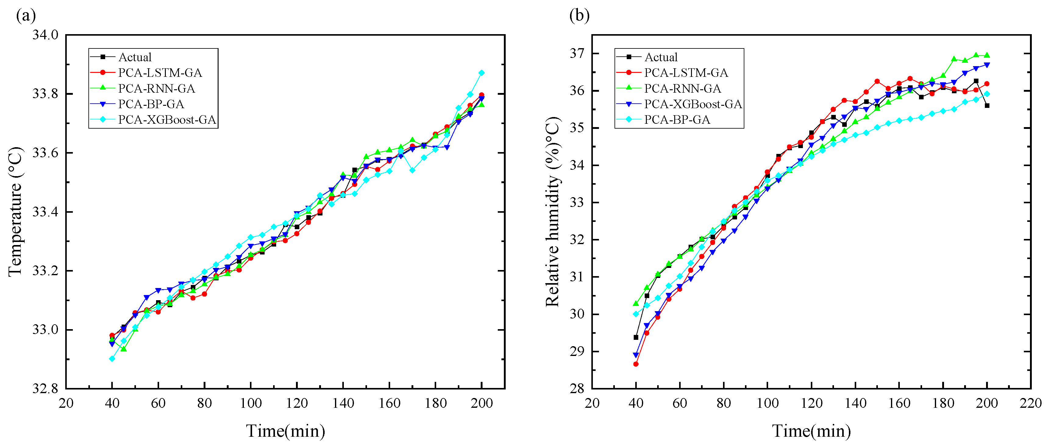
4.3.1. Prediction of Temperature T f o u t at the End of the Roadway

The predicted temperature data on the testing set were compared with the actual temperature data, as shown in Figure 9. Among the 182 pieces of data, 80% were used as the training set, while the other 20% served as the testing set.
The hyperparameters of the LSTM-GA and PCA-LSTM models are disclosed in Table 2.
As presented in Figure 9, the values of MSE and R 2 of the LSTM model are 0.0011 and −0.5724, respectively; those of the LSTM-GA model are 1.6417 × 10⁻⁵ and 0.9762; and those of the PCA-LSTM-GA model are 5.8713 × 10⁻⁶ and 0.9915. Moreover, it can be observed from Figure 9 that the predicted curve of the PCA-LSTM-GA model is the closest to the actual temperature curve.

4.3.2. Prediction of Relative Humidity R H o u t at the End of the Roadway

The predicted humidity data on the testing set were compared with the actual humidity data, as shown in Figure 10. Among the 182 pieces of data, the proportions of the training and test sets were the same as those in Section 4.3.1.
The hyperparameters of the LSTM-GA and PCA-LSTM models are listed in Table 3.
As displayed in Figure 10, the values of MSE and R 2 of the LSTM model are 0.0069 and −0.1504, respectively; those of the LSTM-GA model are 4.1360 × 10⁻⁴ and 0.9314; and those of the PCA-LSTM-GA model are 3.2413 × 10⁻⁴ and 0.9462. Furthermore, it can be observed that the predicted curve of the PCA-LSTM-GA model is the most consistent with the actual humidity curve.

4.3.3. Analysis of Prediction Results

Figure 11 shows how the three models perform in predicting the humidity and temperature at the end of the roadway. As can be discerned, the hybrid learning model optimized by the GA has more excellent performance in predicting the humidity and temperature at the end of the roadway than the single LSTM model. Moreover, after dimension reduction by the PCA, the dimensions of the input features are reduced from 21 to 5 on the basis of reflecting the data feature information to the maximum extent, so the optimization time is decreased significantly in the intelligent optimization by the GA. It is worth mentioning that the prediction performance is not lowered but even improved. This indicates that the PCA algorithm can effectively reduce the interference of data redundancy in model establishment and has an active effect on model optimization.
On the whole, the PCA-GA-LSTM model succeeds in predicting the humidity and temperature at the end of the roadway effectively. The performance of this model can be optimized instantly according to different geological conditions of the roadway, and the hybrid machine learning model has good robustness, so the model is suitable for predicting the humidity and temperature at the end of the roadway.

4.3.4. Comparison of Prediction Results with Other Prediction Models

To further verify the predictive capability of the PCA-LSTM-GA model established in this study, PCA-BP-GA, PCA-XGBOOST-GA, and PCA-RNN-GA models were constructed for comparative tests. Among the 182 pieces of data, the proportions of the training and test sets were the same as those in Section 4.3.2. The prediction curves of all the models are illustrated in Figure 12, and the prediction results of these deep-learning models are disclosed in Table 4.
As can be seen from Table 4, the PCA-LSTM-GA model exhibits the finest prediction capability for both temperature and relative humidity. Moreover, in Figure 12, the prediction curves of the PCA-LSTM-GA model are the closest to the actual change curves, with its error closer to 0 than other models.

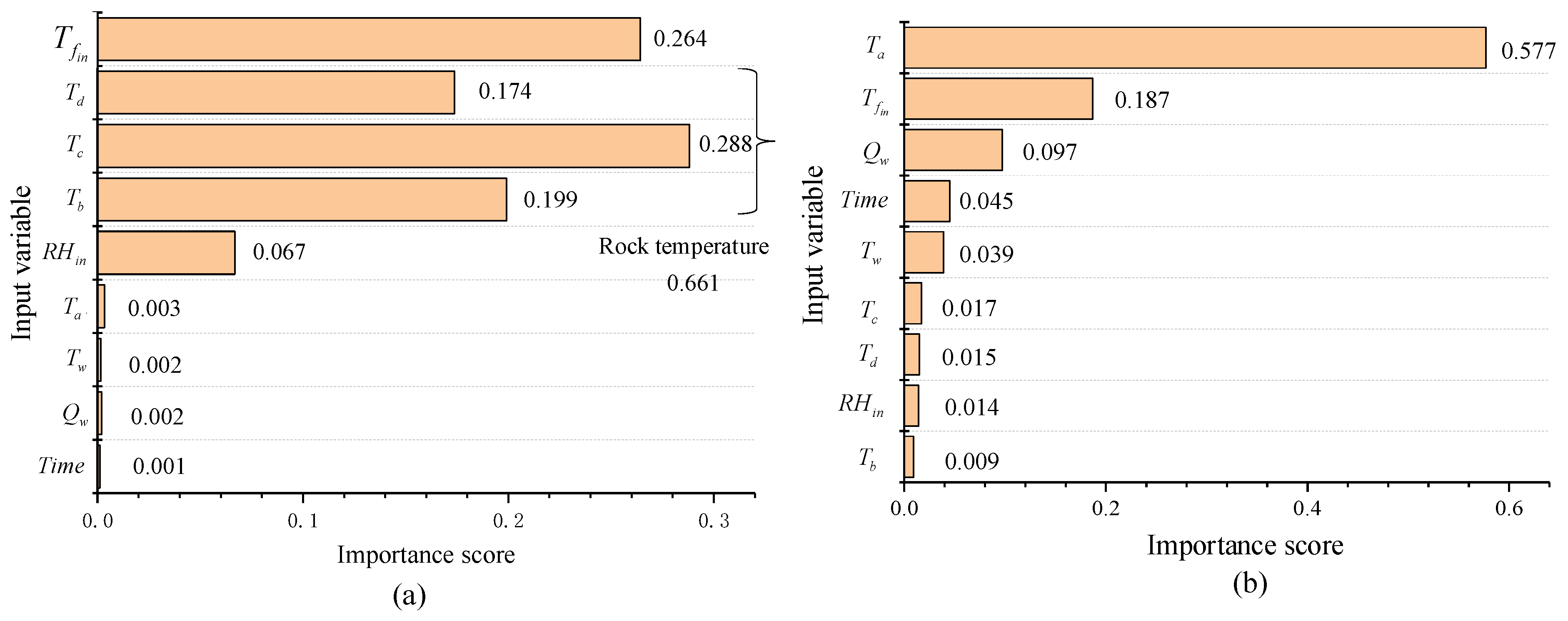
4.4. Variable Importance

To analyze the impact of feature variables on the prediction results of the LSTM model, the partial dependence plot (PDP) method was introduced to explain the output of the model. PDP, a common method for local interpretation [61], visualizes the marginal effect of single features on the prediction results of the LSTM model by taking all the possible values of the input variables as the horizontal axis and the average value of the output variables as the vertical axis, thereby reflecting the impact of different values of important features on the prediction results of the LSTM model. Figure 13 shows the PDPs of the influencing variables T w and Q w , in which the two features do not interact strongly with other model inputs. Clearly, the air temperature T f o u t is directly correlated with the trickling water temperature T w , while T f o u t is inversely related to the trickling water flow rate Q w . The reason is that the heat absorption during evaporation of the trickling water with relatively high flow rate in the roadway causes the conversion of part of the sensible heat in the airflow into latent heat. For prediction of the airflow relative humidity R H o u t , both upwelling water temperature and flow rate are positively correlated with R H o u t , which is expected. In addition, after increasing to a certain extent, the upwelling water temperature and flow rate almost have no influence on the airflow temperature, but start to have evident influence on the airflow humidity. As can be seen from Figure 13, the latent heat and sensible heat variations of airflow in the water upwelling section of roadway are rather complex, so a useful mathematical model can hardly be established to predict the influence of the thermal upwelling water on airflow humidity and temperature at the end of the roadway.
The importance scores (ISs) of input features were calculated in the hope of clarifying their importance. The calculation was conducted using the random forest model based on the mean decrease impurity of modes and depth of the tree for a variable [57,62]. Figure 14a shows the IS results for air temperature T f o u t prediction. Interestingly, the water temperature T w and flow rate Q w have a small influence on the airflow temperature at the end of the roadway, for which the IS is 0.002. The results also indicate that the degrees of importance of the variables to T f o u t follows the order: surrounding rock temperature (IS 0.661) > T f i n (IS 0.264) > R H i n (IS 0.067). This means that, in respect of roadway cooling, researchers and engineers should pay more attention to heat dissipation from surrounding rocks. The roadway airflow temperature accumulates during long-distance transport, and the surrounding rock temperature contributes most of the heat. The shorter the distance of a surrounding rock section to the prediction point, the more important the temperature of this section. For example, the IS of T c is more than that of T b , and T d has a smaller IS than the former two, which may arise from the boundary effect of the model.
Thermal comfort indices, including garment insulation, metabolic rate, radiant heat, airflow rate, air humidity, air temperature, etc., are commonly used to evaluate occupational heat stress risk and to work out adaptation strategies for miners. RH can affect sweat evaporation, as heat rejection from the human body is primarily realized by convective heat transfer. Figure 14b shows the IS results on air RH R H o u t prediction. The results show that the RH R H o u t at the end of the roadway with water trickling is affected by rock temperature in the water upwelling section T a (IS 0.577), inlet airflow temperature T f i n (IS 0.187), upwelling water flow rate Q w (IS 0.097), and upwelling water temperature T w (0.039), and has an evident time effect. The inlet humidity R H i n has a relatively low IS (IS 0.014), which may be caused by the relatively small variation range of R H i n in this experiment.

4.5. Limitations and Superiority

Although the PCA-LSTM-GA model proves to be pretty promising in predicting air humidity and temperature at the end of a water trickling roadway, the following challenges still exist. Firstly, the dataset was acquired from an independently developed modeling roadway which simplified the experimental conditions (e.g., fracture networks). Consequently, the trained model might highly possibly fail to be generalizable to real engineering practice. Secondly, there are still some omissions of other influencing variables for air humidity and temperature prediction, such as wind speed, atmospheric pressure, and ventilation resistance. Thus, for the purpose of ensuring prediction reliability and accuracy, it is necessary to validate and improve the generalization capability after an increasing number of influencing features and data instances are incorporated into the database to ensure the accuracy of prediction.
In this study, a hybrid machine learning (ML) model integrating the PCA-LSTM-GA was proposed for air humidity and temperature prediction. The method requires no thermodynamic parameter tests (e.g., thermal conductivity and heat and mass transfer coefficients) and complex mathematical models once the ML model has been trained. The only thing we need to do is to arrange temperature measurement boreholes in the surrounding rocks at a given interval (Figure 15). The rock temperature values at different depths in boreholes are measured with our independently developed multi-point geo-temperature tester, and the arrangement of temperature sensors is the same as that shown in Figure 3c. The acquired rock temperature data and inlet airflow humidity and temperature data of roadway are transferred to the host computer. If there is thermal water trickling in the roadway, the flow rate and temperature need to be processed for equivalence.
Another enlightenment given to us by this study is that the thermal water trickling into the roadway, which damages the workers’ operation comfort, cannot be ignored. For this type of roadway, we proposed that a composite heat insulation structure with heat insulation and support for the roadway should be arranged. Concrete is sprayed onto the stable roadway walls first, and then heat insulation materials are filled into the loose ring of surrounding rock through grouting anchor cable or anchor rod to block the fracture water. Afterwards, heat insulation materials are sprayed onto the outside of the concrete layer. Finally, concrete is sprayed onto the outermost layer. This method can effectively reduce the heat conduction and convection between rock mass and thermal water.

5. Conclusions

In this study, a ML and GA-based intelligent modeling framework was proposed for predicting air humidity and temperature at the end of the water trickling roadway. Twenty-one features were chosen as input variables. More than 200 pieces of data were collected from an independently developed modeling roadway to construct the dataset, in particular, the thermal water and flow rate were taken into comprehensive consideration first for training and validating of the LSTM, LSTM-GA, and PCA-LSTM-GA models. The thermal system enthalpy difference, MSE and R 2 were chosen as the assessment indices. Several conclusions are summarized as follows.
(1)
Thermal water trickling into the roadway can evidently change the enthalpy of the thermal system. The increase in upwelling water flow rate induces a linear rise of the enthalpy difference of humid air, but it barely affects the sensible heat of air. The increase in upwelling water temperature influences both the latent heat and sensible heat of air. As a result, the total enthalpy difference of the humid air rises nonlinearly.
(2)
The PCA-LSTM-GA model is robust in predicting the air humidity and temperature at the end of the trickling roadway. LSTM is suitable for processing time series data. GA is efficient in hyperparameter tuning of the LSTM. PCA optimizes the hybrid model, raising its convergence speed and bringing about an increase in R 2 .
(3)
As demonstrated by the importance scores, the airflow temperature at the end of the water trickling roadway is mainly influenced by the surrounding rock temperature (IS 0.661) and inlet airflow temperature (IS 0.264). The airflow humidity at the end of the roadway with water trickling is mainly influenced by the rock temperature in water upwelling section (IS 0.577), inlet airflow temperature (IS 0.187), and upwelling water temperature and flow rate (total IS 0.136), and it has an evident time effect. The enlightenment given to us is that, for thermal control for this type of roadway, a composite heat insulation structure with jet grouting and support techniques for heat insulation should be arranged.
In future work, the generalization of the proposed model can be promoted through employing a larger dataset with multiple variables. Moreover, we have developed relevant equipment and have an engineering practice method to apply the ML model.

Author Contributions

Data curation, Z.J.; writing—original draft preparation, J.W.; writing—review and editing, D.W. and Y.Z. All authors have read and agreed to the published version of the manuscript.

Funding

This research received no external funding.

Institutional Review Board Statement

Not applicable.

Informed Consent Statement

Not applicable.

Data Availability Statement

The data presented in this study are available upon request from the corresponding author. The data are not publicly available due to privacy.

Conflicts of Interest

The authors declare no conflict of interest.

Abbreviations

RH = Relative humidity; LSTM = Long short-term memory; GA = Genetic algorithm; PCA = Principal component analysis; IS = Importance scores; MIV = Mine intelligent ventilation; FEM = Finite element method; FVM = Finite Volume Method; ML = Machine learning; HGT = high geo-temperature; TWUT = Thermal water upwelling and trickling; EAHMT = Experimental apparatus for heat and mass transfer; SRHS = Surrounding rock heating system; CTHV = Constant temperature and humidity ventilator; RNN = Recurrent neural network; MSE = Mean Square Error; PDP = Partial dependence plot.

References

  1. Sunkpal, M.; Roghanchi, P.; Kocsis, K.C. A Method to Protect Mine Workers in Hot and Humid Environments. Saf. Health Work 2017, 9, 149–158. [Google Scholar] [CrossRef] [PubMed]
  2. Han, Q.; Zhang, Y.; Li, K.; Zou, S. Computational evaluation of cooling system under deep hot and humid coal mine in China: A thermal comfort study. Tunn. Undergr. Space Technol. 2019, 90, 394–403. [Google Scholar]
  3. Yang, X.; Han, Q.; Pang, J.; Shi, X.; Hou, D.; Liu, C. Progress of heat-hazard treatment in deep mines. Min. Sci. Technol. 2011, 21, 295–299. [Google Scholar]
  4. Zhang, Y.; Wan, Z.J.; Gu, B.; Zhou, C.B.; Cheng, J.Y. Unsteady temperature field of surrounding rock mass in high geothermal roadway during mechanical ventilation. J. Cent. South Univ. 2017, 24, 374–381. [Google Scholar] [CrossRef]
  5. Wang, J.; Wan, Z.; Zhang, H.; Wu, D.; Zhang, Y.; Wang, Y.; Xiong, L.; Wang, G. Application of Thermal Insulation Gunite Material to the High Geo-Temperature Roadway. Adv. Civ. Eng. 2020, 2020, 8853870. [Google Scholar] [CrossRef]
  6. Wan, Z.; Bi, S.; Zhang, Y.; Wang, J.; Wu, D.; Wang, J. Framework of the theory and technology for simultaneous extraction of coal and geothermal resources. J. China Coal Soc. 2018, 43, 2099–2106. [Google Scholar]
  7. Ji, J.; Li, N.; Chang, Z.; Fan, Y.; Ni, L. Study on heat transfer characteristic parameters and cooling effect of cold wall cooling system in coal mines. Exp. Heat Transf. 2020, 33, 179–196. [Google Scholar] [CrossRef]
  8. He, M. Application of HEMS cooling technology in deep mine heat hazard control. Min. Sci. Technol. 2009, 19, 269–275. [Google Scholar] [CrossRef]
  9. Zhou, F.B.; Wei, L.J.; Xia, T.Q.; Wang, K.; Wu, X.Z.; Wang, Y.M. Principle, key technology and preliminary realization of mine intelligent ventilation. J. China Coal Soc. 2020, 45, 2225–2235. [Google Scholar]
  10. Zhang, Y.; Wan, Z.; Ma, Z.; Gu, B.; Ma, Y. Heat transfer analysis of surrounding rocks with thermal insulation layer in high geothermal roadway. Therm. Sci. 2017, 23, 178. [Google Scholar] [CrossRef]
  11. Шepбaнь, H.; Huang, H. Guidelines for Mine Cooling; Coal Industry Press: Beijing, China, 1982. (In Chinese) [Google Scholar]
  12. Cen, Y.Q.; Hu, C.S.; Hou, Q.Z. Investigation into unsteady heat transfer coefficient K between the surrounding rock of mine wells or lanes and airflow. J. Liaoning Tech. Univ. 1987, 3, 14. [Google Scholar]
  13. Zhou, X.H.; Shan, Y.F.; Wang, J.R. The Unsteady Thermal Exchange between Wall Rock and Airflow of Roadway. J. Liaoning Tech. Univ. (Nat. Sci. Ed.) 2002, 3, 264–266. [Google Scholar]
  14. Sun, P. A New Method for Calculating the Instable Heat Transfer Coefficient. J. China Univ. Min. Technol. 1991, 2, 36–40. [Google Scholar]
  15. Yakovenko, A.K.; Averin, G.V. Determination of the heat-transfer coefficient for a rock mass with small fourier numbers. J. Min. Sci. 1984, 20, 52–56. [Google Scholar] [CrossRef]
  16. Wang, Y.J.; Zhou, G.Q.; Wu, L. Unsteady heat-moisture transfer of wet airway in deep mining. J. Cent. South Univ. 2013, 20, 1971–1977. [Google Scholar] [CrossRef]
  17. Qin, Y. Computing the Unsteady-state Heat Transfer Criterion Between Air and Rock Surrounding Airway with Finite Difference Method. J. Xiangtan Min. Inst. 1998, 13, 6–10. [Google Scholar]
  18. Roy, T.R.; Singh, B. Computer simulation of transient climatic conditions in underground airways. Min. Sci. Technol. 1991, 13, 395–402. [Google Scholar] [CrossRef]
  19. Zhu, S.; Wu, S.; Cheng, J.; Li, S.; Li, M. An Underground Air-Route Temperature Prediction Model for Ultra-Deep Coal Mines. Minerals 2015, 5, 527–545. [Google Scholar] [CrossRef]
  20. Wang, F.; Luo, F.; Huang, Y.; Zhu, L.; Hu, H. Thermal analysis and air temperature prediction in TBM construction tunnels. Appl. Therm. Eng. 2019, 158, 113822. [Google Scholar] [CrossRef]
  21. Yao, W.; Pang, J.; Ma, Q.; Lyimo, H. Influence and sensitivity analysis of thermal parameters on temperature field distribution of active thermal insulated roadway in high temperature mine. Int. J. Coal Sci. Technol. 2020, 8, 47–63. [Google Scholar] [CrossRef]
  22. Zhang, S.; Lu, P.; Wang, H. Numerical Simulation Analysis of Unsteady Temperature in Thermal Insulation Supporting Roadway. Math. Probl. Eng. 2019, 2019, 6279164. [Google Scholar] [CrossRef]
  23. Nie, X.; Feng, S.; Shudu, Z.; Quan, G. Simulation study on the dynamic ventilation control of single head roadway in high-altitude mine based on thermal comfort. Adv. Civ. Eng. 2019, 2019, 2973504. [Google Scholar] [CrossRef]
  24. Wang, J. Geothermal and Its Applications; Science Press: Beijing, China, 2015. [Google Scholar]
  25. Janson, E.; Boyce, A.J.; Burnside, N.; Gzyl, G. Preliminary investigation on temperature, chemistry and isotopes of mine water pumped in Bytom geological basin (USCB Poland) as a potential geothermal energy source. Int. J. Coal Geol. 2016, 164, 104–114. [Google Scholar] [CrossRef]
  26. Wang, Q.; Wang, X.; Hou, Q. Geothermal Water at a Coal Mine: From Risk to Resource. Mine Water Environ. 2015, 35, 294. [Google Scholar] [CrossRef]
  27. Liu, H.Q.; Wang, H.; Shao, X.W. Analysis and a simplified calculation method of the thermo-moisture exchange between the hot mining roadway wall and the airflow. J. Saf. Environ. 2012, 12, 208–212. [Google Scholar]
  28. Gao, J.L.; Xu, W.; Zhang, X.B. Treatment of water evaporation during calculation of temperature and humidity of airflow caused by heat release from surrounding rock. J. China Coal Soc. 2010, 35, 951–955. [Google Scholar]
  29. Li, Z.; Wang, T.M.; Zhang, M.Q.; Jia, J.; Lin, L. Construction of air flow heat transfer coefficient and calculation of airflow temperature in mine wet roadway. J. China Coal Soc. 2017, 42, 3176–3181. [Google Scholar]
  30. Yu, X.; Zijun, L.; Junjian, W.; Yin, C.; Huasen, L.; Wei, P.; Mintao, J. Research on simulation experiment for synergetic mining of geothermal energy to heat hazard control. J. Cent. South Univ. (Sci. Technol.) 2023, 54, 2162–2173. [Google Scholar]
  31. Li, Z.; Xu, Y.; Jia, M.; Liu, H.; Pan, W.; Deng, Y. Numerical simulation on heat hazard control by collaborative. J. Central South Univ. (Sci. Technol.) 2021, 52, 671–680. [Google Scholar]
  32. Zhang, Z.; Wang, S.H.; Yin, H.; Yang, T.J.; Wang, P.Y. Fracture seepage and the temperature field distribution of rocks surrounding high-temperature tunnels: A numerical analysis. Geomech. Geophys. Geo-Energy Geo-Resour. 2022, 8, 30. [Google Scholar] [CrossRef]
  33. Sun, Y.; Zhang, J.; Li, G.; Ma, G.; Huang, Y.; Sun, J.; Nener, B. Determination of Young’s modulus of jet grouted coalcretes using an intelligent model. Eng. Geol. 2019, 252, 43–53. [Google Scholar] [CrossRef]
  34. Zhang, J.; Li, D.; Wang, Y. Predicting tunnel squeezing using a hybrid classifier ensemble with incomplete data. Bull. Eng. Geol. Environ. 2020, 79, 3245–3256. [Google Scholar] [CrossRef]
  35. Sun, Y.; Zhang, J.; Li, G.; Wang, Y.; Sun, J.; Jiang, C. Optimized neural network using beetle antennae search for predicting the unconfined compressive strength of jet grouting coalcretes. Int. J. Numer. Anal. Methods Geomech. 2019, 43, 801–813. [Google Scholar] [CrossRef]
  36. Wu, Y.; Gao, R.; Yang, J. Prediction of coal and gas outburst: A method based on the BP neural network optimized by GASA. Process Saf. Environ. Prot. 2019, 133, 64–72. [Google Scholar] [CrossRef]
  37. Zhao, D.; Wu, Q.; Cui, F.; Xu, H.; Zeng, Y.; Cao, Y.; Du, Y. Using random forest for the risk assessment of coal-floor water inrush in Panjiayao Coal Mine, northern China. Hydrogeol. J. 2018, 26, 2327–2340. [Google Scholar] [CrossRef]
  38. Tan, T.; Yang, Z.; Chang, F.; Zhao, K. Prediction of the First Weighting from the Working Face Roof in a Coal Mine Based on a GA-BP Neural Network. Appl. Sci. 2019, 9, 4159. [Google Scholar] [CrossRef]
  39. Jo, B.; Khan, R. An internet of things system for underground mine air quality pollutant prediction based on azure machine learning. Sensors 2018, 18, 930. [Google Scholar] [CrossRef] [PubMed]
  40. Yin, Q.; Liu, R.; Jing, H.; Su, H.; Yu, L.; He, L. Experimental Study of Nonlinear Flow Behaviors Through Fractured Rock Samples After High-Temperature Exposure. Rock Mech. Rock Eng. 2019, 52, 2963–2983. [Google Scholar] [CrossRef]
  41. Yin, Q.; Wu, J.; Zhu, C.; He, M.; Meng, Q.; Jing, H. Shear mechanical responses of sandstone exposed to high temperature under constant normal stiffness boundary conditions. Geomech. Geophys. Geo-Energy Geo-Resour. 2021, 7, 35. [Google Scholar] [CrossRef]
  42. Yin, Q.; Wu, J.; Zhu, C.; Wang, Q.; Zhang, Q.; Jing, H.; Xie, J. The role of multiple heating and water cooling cycles on physical and mechanical responses of granite rocks. Geomech. Geophys. Geo-Energy Geo-Resour. 2021, 7, 69. [Google Scholar] [CrossRef]
  43. Li, L.; Chang, F. Prediction and Application of Temperature and Humidity of Airflow in Deep and Long Tunnel. J. Highw. Transp. Res. Dev. 2021, 38, 110–116. [Google Scholar]
  44. Bascompta, M.; Rossell, J.M.; Sanmiquel, L.; Anticoi, H. Temperature Prediction Model in the Main Ventilation System of an Underground Mine. Appl. Sci. 2020, 10, 7238. [Google Scholar] [CrossRef]
  45. Wang, Y.J.; Zhou, G.Q.; Wei, Y.Z.; Kuang, L.F.; Wu, L. Experimental research on changes in the unsteady temperature field of an airway in deep mining engineering. J. China Univ. Min. Technol. 2011, 40, 345–350. [Google Scholar]
  46. Zhang, Y.; Wan, Z.; Gu, B.; Zhou, C. An experimental investigation of transient heat transfer in surrounding rock mass of high geothermal roadway. Therm. Sci. 2016, 20, 2149–2158. [Google Scholar] [CrossRef]
  47. Lever, J.; Krzywinski, M.; Altman, N. Points of Significance: Principal component analysis. Nat. Methods 2017, 14, 641–642. [Google Scholar] [CrossRef]
  48. de Almeida, F.A.; Santos AC, O.; de Paiva, A.P.; Gomes, G.F.; Gomes, J.H.D.F. Multivariate Taguchi loss function optimization based on principal components analysis and normal boundary intersection. Eng. Comput. 2020, 38, 1627–1643. [Google Scholar] [CrossRef]
  49. Liu, Y.; Liu, Y.; Zhang, Q.; Li, C.; Feng, Y.; Wang, Y.; Ma, H. Petrophysical static rock typing for carbonate reservoirs based on mercury injection capillary pressure curves using principal component analysis. J. Pet. Sci. Eng. 2019, 181, 106175. [Google Scholar] [CrossRef]
  50. Hochreiter, S.; Schmidhuber, J. Long Short-Term Memory. Neural Comput. 1997, 9, 1735–1780. [Google Scholar] [CrossRef]
  51. Palangi, H.; Deng, L.; Shen, Y.; Gao, J.; He, X.; Chen, J.; Song, X.; Ward, R. Deep Sentence Embedding Using Long Short-Term Memory Networks: Analysis and Application to Information Retrieval. IEEE/ACM Trans. Audio Speech Lang. Process. 2016, 24, 694–707. [Google Scholar] [CrossRef]
  52. Ma, J.; Ding, Y.; Cheng, J.C.; Jiang, F.; Wan, Z. A Temporal-Spatial Interpolation and Extrapolation Method Based on Geographic Long Short-Term Memory Neural Network for PM2.5. J. Clean. Prod. 2019, 237, 117729. [Google Scholar] [CrossRef]
  53. Yin, Z.Y.; Jin, Y.F.; Huang, H.W.; Shen, S.L. Evolutionary polynomial regression based modelling of clay compressibility using an enhanced hybrid real-coded genetic algorithm. Eng. Geol. 2016, 210, 158–167. [Google Scholar] [CrossRef]
  54. Park, H.I.; Kim, K.S.; Kim, H.Y. Field performance of a genetic algorithm in the settlement prediction of a thick soft clay deposit in the southern part of the Korean peninsula. Eng. Geol. 2015, 196, 150–157. [Google Scholar] [CrossRef]
  55. Qi, C.; Chen, Q.; Fourie, A.; Zhang, Q. An intelligent modelling framework for mechanical properties of cemented paste backfill. Miner. Eng. 2018, 123, 16–27. [Google Scholar] [CrossRef]
  56. Lingaraj, H. A Study on Genetic Algorithm and its Applications. Int. J. Comput. Sci. Eng. 2016, 4, 139–143. [Google Scholar]
  57. Tian, J.; Qi, C.; Sun, Y.; Yaseen, Z.M.; Pham, B.T. Permeability prediction of porous media using a combination of computational fluid dynamics and hybrid machine learning methods. Eng. Comput. 2020, 37, 3455–3471. [Google Scholar] [CrossRef]
  58. Bacardit, A.; Morera, J.M.; Ollé, L.; Bartolí, E.; Dolors, B.M. Mine Ventilation and Air Conditioning, 3rd ed.; John Wiley & Sons: Hoboken, NJ, USA, 1961. [Google Scholar]
  59. Qasem, S.N.; Samadianfard, S.; Nahand, H.S.; Mosavi, A.; Shamshirband, S.; Chau, K.W. Estimating Daily Dew Point Temperature Using Machine Learning Algorithms. Water 2019, 11, 582. [Google Scholar] [CrossRef]
  60. Zhang, J.; Sun, Y.; Li, G.; Wang, Y.; Sun, J.; Li, J. Machine-learning-assisted shear strength prediction of reinforced concrete beams with and without stirrups. Eng. Comput. 2020, 38, 1293–1307. [Google Scholar] [CrossRef]
  61. Friedman, J.H. Greedy Function Approximation: A Gradient Boosting Machine. Ann. Stat. 2001, 29, 1189–1232. [Google Scholar] [CrossRef]
  62. Qi, C.; Fourie, A.; Chen, Q.; Zhang, Q. A strength prediction model using artificial intelligence for recycling waste tailings as cemented paste backfill. J. Clean. Prod. 2018, 183, 566–578. [Google Scholar] [CrossRef]
Figure 1. Microclimate conditions of Sanhejian Coal Mine: (a) airflow path at the A-Ⅰ working face; (b) geothermal temperature isogram at the depth of −700 m; (c) deep circulating thermal water upwelling and trickling (TWUT) to roadway; (note: route 2–8 is −700 m main auxiliary roadway; route 8–12 is track rise; route 12–13 is head entry; route 13–14 is A-Ⅰ working face; route 14–15 is tail entry).
Applsci 13 13343 g001
Figure 2. Measuring result of mine microclimate parameters: (a) Temperature measurements; (b) Enthalpy measurements.
Applsci 13 13343 g002
Figure 3. The composition sketch map of the EAHMT and arrangement of sensors: (a) the composition sketch map; (b) A-A profile of the modeling roadway; (c) B-B profile of the modeling roadway.
Applsci 13 13343 g003
Figure 4. Dynamic variation curves of dimensionless temperature at various points of surrounding rocks in the radial direction with time (note: T f denotes the airflow temperature).
Applsci 13 13343 g004
Figure 5. LSTM neural structure.
Applsci 13 13343 g005
Figure 7. Total enthalpy difference variations in a roadway with water trickling at different water temperatures (a) and flow rates (b).
Applsci 13 13343 g007
Figure 8. Hyperparameters tuning using GA model for (a) temperature T f o u t prediction and (b) relative humidity R H o u t prediction.
Applsci 13 13343 g008
Figure 9. Comparison between predicted and actual temperatures T f o u t on the testing set among the three models. (a) LSTM. (b) LSTM-GA. (c) PCA-LSTM-GA.
Applsci 13 13343 g009
Figure 10. Comparison between predicted and actual relative humidities R H o u t on the testing set among the three models. (a) LSTM. (b) LSTM-GA. (c) PCA-LSTM-GA.
Applsci 13 13343 g010
Figure 11. Comparison of errors among the three models. (Note: A 1 , A 2 , A 3 denote the prediction of temperature T f o u t by the LSTM, LSTM-GA, and PCA-LSTM-GA, respectively; B 1 , B 2 , B 3 denote the prediction of relative humidity R H o u t by the LSTM, LSTM-GA, and PCA-LSTM-GA, respectively).
Applsci 13 13343 g011
Figure 12. Comparison of prediction curves of different prediction models for: (a) temperature; (b) relative humidity.
Applsci 13 13343 g012
Figure 13. Partial dependence plots of water temperature T w and flow rate Q w for predicting air temperature T f o u t (a,b) and air RH R H o u t (c,d) at the end of the roadway with water trickling.
Applsci 13 13343 g013
Figure 14. Importance scores of input variables for (a) air temperature T f o u t and (b) air RH R H o u t prediction.
Applsci 13 13343 g014
Figure 15. Application of PCA-LSTM-GA model.
Applsci 13 13343 g015
Table 1. Descriptive statistics regarding input and output.
ParameterMean ValueStandard DeviationMin ValueMax Value
τ (min)97 5205
Q w (mL/min)125 50200
T w (°C)60 4080
T a (°C)37.81.434.342.2
T f i n (°C)23.00.821.024.2
T b (°C)41.31.239.443.2
T c (°C)45.41.243.447.2
T d (°C)44.81.542.546.9
R H i n (%)21.02.516.725.4
R H o u t (%)26.27.712.840.2
T f o u t (°C)34.32.528.237.4
Note: to facilitate statistics, the surrounding rock temperature was taken as the mean value in cylinders a–d, and T a means the mean value of T a 1 T a 4 .
Table 2. Optimal hyperparameters of the models for temperature prediction.
Number of Units in LSTM LayerBatch SizeOptimizer Learning RateDropout Layer Parameter
LSTM-GA78110.00681950.283
PCA-LSTM-GA34200.0017590.151
Table 3. Optimal hyperparameters of the models for relative humidities prediction.
Number of Units in LSTM LayerBatch SizeOptimizer Learning RateDropout Layer Parameter
LSTM-GA42200.006540.254
PCA-LSTM-GA16210.0092530.1163
Table 4. Error of prediction results of different models.
Prediction ModelTemperatureRelative Humidity
MSER2MSER2
PCA-LSTM-GA5.871310 × 10−60.99153.2413 × 10−40.9462
PCA-RNN-GA7.2956 × 10−60.98623.3891 × 10−40.9407
PCA-BP-GA8.4125 × 10−60.98413.5692 × 10−40.9359
PCA-XGBoost-GA2.16435 × 10−60.96173.7128 × 10−40.9243
Disclaimer/Publisher’s Note: The statements, opinions and data contained in all publications are solely those of the individual author(s) and contributor(s) and not of MDPI and/or the editor(s). MDPI and/or the editor(s) disclaim responsibility for any injury to people or property resulting from any ideas, methods, instructions or products referred to in the content.

