Leveraging Ensemble Learning with Generative Adversarial Networks for Imbalanced Software Defects Prediction

Abstract

Software defect prediction is an active research area. Researchers have proposed many approaches to overcome the imbalanced defect problem and build highly effective machine learning models that are not biased towards the majority class. Generative adversarial networks (GAN) are one of the state-of-the-art techniques that can be used to generate synthetic samples of the minority class and produce a balanced dataset. However, it was not investigated thoroughly in the area of imbalanced defect prediction. In this paper, we proposed to combine GAN-based methods with boosting ensembles to yield robust defect prediction models. GAN-based methods were used to balance the defect datasets, and the AdaBoost ensemble was employed to classify the modules into defective and non-defective modules. Our proposed approach was investigated within the context of 10 software defect datasets with different imbalance ratios. Wilcoxon effect size and Scott–Knott effect size difference tests were used as statistical tests to quantify the model’s performance differences statistically. Empirical results indicated that GAN-based methods need hyperparameter optimization when used for imbalanced software defect prediction. In comparison to the traditional sampling techniques, GAN methods outperformed all traditional techniques when used for imbalanced defect prediction. Lastly, results demonstrated that GAN-based methods should not be combined with undersampling to handle imbalance problems.

1. Introduction

Nowadays, several modern software systems have been developed to meet consumers’ increasing demands. Due to the growing number of modern software systems, software reliability has become a critical issue, with modern software being complex and highly defect-prone [1]. Early defect prediction helps in improving the planning and execution of software development projects. Software defects are the main cause of software failures and can cause serious issues (e.g., financial loss) [2]. Therefore, systems developers need to put a considerable amount of effort into testing and debugging to improve overall software reliability. Manual software defect reviews require more time and effort and can detect only 60% of software defects [3].

Many researchers have successfully employed machine learning models in the software defect prediction process to achieve a better prediction performance and reduce the consumed time and effort [4]. However, these models yield a biased performance on imbalanced software defect datasets towards majority class samples. The number of defective modules (minority class) in imbalanced datasets is much lower than the number of non-defective modules (majority class). In order to handle the class imbalance, several techniques could be employed that can be categorized into different levels, such as data-level, cost-sensitive, ensemble learning, and hybrid-level techniques.

In this paper, we focus on the data-level and ensemble-learning techniques to handle the software defect imbalance problem. We aim to combine GAN-based methods with boosting ensemble learning to deal with the imbalance issue and enhance the software defect prediction. Our paper’s main contributions are: (1) to propose a hybrid approach that can deal with the software defect imbalance problem efficiently by combining GAN-based methods with boosting ensembles and (2) to empirically validate the proposed approach by conducting a comprehensive empirical study to study the effectiveness of our proposed approach against traditional oversampling and undersampling approaches.

Combining GAN with boosting ensembles has never been investigated in previous software defect prediction studies. Therefore, our main objective in this paper is to develop an approach that combines GAN-based methods with boosting ensembles to address the software defect imbalance problem and enhance overall defect prediction. This approach takes advantage of boosting ensembles and GAN models by employing GAN to generate synthetic samples of the minority class and employs the boosting ensemble to perform the classification task into defective and non-defective modules. To achieve our research objective, we formulated the following research questions:

• RQ1: Will hyperparameter optimization of GAN-based methods yield enhanced defect prediction performance over default hyperparameters?
• RQ2: Will utilizing GAN-based methods yield enhanced defect prediction performance over traditional undersampling and oversampling techniques?
• RQ3: Will combining GAN-based methods with undersampling yield enhanced defect prediction performance?

The remaining sections of this paper are organized as follows. Section 2 provides a brief background of the main techniques used in this study. Section 3 discusses the literature review and presents the gap analysis. Section 4 describes the proposed approach for handling imbalance issues in software defect datasets. Section 5 describes the empirical study that we conducted, whereas Section 6 presents and discusses the results of this study. Finally, Section 7 concludes the paper, presents the contributions of this work, and provides direction for future work.

2. Background

This section presents a general background of the main techniques that are used in this study.

2.1. Generative Adversarial Networks

A generative adversarial network (GAN) is a type of adversarial training system that was first proposed in 2014 by Goodfellow et al. [5]. It contains two networks trained against each other; the first network is called a generator, and the second network is called a discriminator. The generator is responsible for capturing the real distribution of the data and generating synthetic samples. It takes a random noise as input and generates fake data, whereas the discriminator is considered a simple binary classifier that classifies the samples into fake or real. It takes two inputs, which are real data from the original dataset and fake data from the generator [5].

The generator and discriminator act like competitors. The generator tries to fool the discriminator by generating samples similar to real samples, while the discriminator tries to classify the samples as real or fake. The generator can not access the real data directly. Instead, there is an interaction between the generator and the discriminator. Hence, based on this interaction, the generator keeps trying to generate data of better quality. The interaction between the generator and discriminator can be thought of as a minimax game. Equation (1) presents the minimax loss function, which is based on the Jensen–Shannon Divergence (JSD). The generator is trained in order to decrease $\log (1-D(G\left(z\right)\left)\right)$, while the discriminator is trained in order to increase $\log D\left(x\right)+\log (1-D(G\left(z\right)\left)\right)$.

$$\underset{G}{min}\underset{D}{max}{\mathbb{E}}_{\mathit{x}\sim p_{\mathrm{data}}}\left[\log D\left(\mathit{x}\right)\right]+{\mathbb{E}}_{\mathit{z}\sim p_{\mathit{z}}}\left[\log (1-D\left(G\left(\mathit{z}\right)\right))\right]$$

(1)

where:

• $E\left(x\right)$ is the expected value across all samples (x) of real data.
• $\log D\left(x\right)$ is the probability that the discriminator correctly classified real data.
• $E\left(z\right)$ is the expected value across all samples of generated data.
• $G\left(z\right)$ is the generated sample when z is the random input noise to the generator.
• $\log D\left(G\right(z\left)\right)$ is the probability that the discriminator correctly classified generated data.

The discriminator remains fixed during generator training and vice versa. The discriminator is connected to the generator and discriminator loss functions. The discriminator loss function is used during discriminator training. If the discriminator classifies fake data as real or real data as fake, it penalizes itself using the loss function. Through backpropagation, the discriminator loss function is used to update the weights of the discriminator network. The generator loss function is used during the generator training. If the discriminator correctly classifies the input, the generator penalizes itself through the generator loss. As training progresses, the generator produces better results that can fool the discriminator [5].

2.2. Conditional Generative Adversarial Networks

Original GAN suffers a key problem, which is mode-collapse. Mode collapse occurs when the generator generates a set of samples that successfully fool the discriminator. Thus, the generator will keep generating the same set of outputs, and the discriminator will not provide a useful gradient to the generator [6]. Therefore, Wasserstein GAN (WGAN) was proposed to force the discriminator to provide an informative gradient. WGAN uses Wasserstein distance with 1-Lipschitz constraint instead of the JSD in the minimax loss. In WGAN, weight clipping is used to force the 1-Lipschitz constraint on the discriminator function. Weight clipping can be defined as clipping the discriminator weights to lie in the range [−c, c], where c is a given hyperparameter. Weight clipping is applied to all layers of the discriminator network to enforce 1-Lipschitz. In WGAN, the discriminator does not classify the samples as real or fake. Instead, it returns a score that implies the distance between real and generated samples. Therefore, the discriminator in WGAN is called critic [6]. Equation (2) presents the Wasserstein loss function.

$$\underset{G}{min}\underset{D}{max}{\mathbb{E}}_{\mathit{x}{p}_{\mathrm{data}}}\left[D\left(\mathit{x}\right)\right]-{\mathbb{E}}_{\mathit{z}\sim p_{\mathit{z}}}\left[D\left(G\left(\mathit{z}\right)\right)\right]$$

(2)

WGAN with weight clipping still suffers from two problems: vanishing gradient and exploding gradient [6]. To overcome the problems of WGAN, a gradient penalty can be used instead of weight clipping. The critic function is 1-Lischitz if and only if its gradient is at most 1 [6]. In general, the gradient penalty is the squared difference between the linear interpolations and 1. Equation (3) presents the Wasserstein loss with gradient penalty. Conditional WGANGP (CWGANGP) combines conditional GAN (CGAN) with WGANGP to enable WGANGP to produce conditioned data. CGAN is a simple variant of GAN that adds a conditional vector to the generator and discriminator to generate data with specified class labels [6].  

$$\underset{G}{min}\underset{D}{max}{\mathbb{E}}_{\mathit{x}\sim p_{\mathrm{data}}}\left[D\left(\mathit{x}\right)\right]-{\mathbb{E}}_{\mathit{z}\sim p_{\mathit{z}}}\left[D\left(G\left(\mathit{z}\right)\right)\right]+\lambda {\mathbb{E}}_{\widehat{\mathit{x}}\sim p_{\widehat{\mathit{x}}}}\left[{\left({∥{\nabla }_{\widehat{x}}D\left(\widehat{x}\right)∥}_2-1\right)}^2\right]$$

(3)

where:

• $\lambda$ is the gradient coefficient.
• $\widehat{x}$ is the linear interpolations between the generated and real samples.

2.3. Conditional Tabular Generative Adversarial Networks

Tabular datasets usually include a mix of continuous and discrete variables. Thus, capturing the distribution of these datasets using GAN is not a trivial process. Therefore, a Conditional Tabular Generative Adversarial Network (CTGAN) was proposed in 2019 to deal with tabular data [7]. CTGAN differs from the original GAN in many aspects. Firstly, it uses mode-specific normalization to deal with non-gaussian distribution and multimodel data. In the mode-specific normalization process, each continuous column is processed separately. The Variational Gaussian Mixture model (VGM) is used to find the number of modes in each column. Then, the Gaussian mixture model is fitted. The learned Gaussian mixture is ${\mathbb{P}}_{c_i}\left(c_{i,j}\right)={\sum }_{k=1}^l{\mu }_k\mathbb{N}\left(c_{i,j};{\eta }_k,{\varphi }_k\right)$ where ${\mu }_k$ is the weight of a mode $\left(k\right)$ and ${\varphi }_k$ is the standard deviation of the mode. The probability density for each mode of the value in the column is calculated as follows: ${\rho }_k={\mu }_k\mathbb{N}\left(c_{i,j};{\eta }_k,{\varphi }_k\right)$. Then each value $c_{i,j}$ in each mode is represented as a one-hot vector $\left({\beta }_{i,j}\right)$ of size equal to the number of modes. Additionally, a scalar value $\left({\alpha }_{i,j}\right)$ is utilized to represent the value $c_{i,j}$. Thus, each row in the dataset is represented as follows:

$$r_j={\alpha }_{1,j}\oplus {\beta }_{1,j}\oplus \dots \oplus {\alpha }_{N_c,j}\oplus {\beta }_{N_c,j}\oplus d_{1,j}\oplus d_{N_c,j}$$

(4)

where d is the representation of discrete columns [7].

Furthermore, a conditional vector is constructed and provided as an input to the generator with the random noise vector. Suppose we have two discrete columns $D_1$ and $D_2$. Let $D_1=\{1,2,3\}$, $D_2=\{1,2\}$ and the given condition is $D_2=1$. The conditional vector will be the concatenation of all discrete columns, where all values are represented as 0, and the condition is represented as 1. Thus, the conditional vector will be $m=[0,0,0,1,0]$. To enforce the given condition, a cross-entropy loss is used between the generated sample and the conditional vector. In CTGAN architecture, fully connected layers were used to capture all possible relations between columns. Also, CTGAN uses PacGAN architecture in the discriminator to mitigate the mode-collapse problem in the original GAN. In addition, it utilizes the Wasserstein loss function with gradient penalty to train the model [7].

2.4. Traditional Sampling Techniques

There are many classical and traditional sampling techniques that exist to handle imbalanced datasets, such as Random oversampling (ROS), Random undersampling (RUS), and Synthetic Minority Oversampling Technique (SMOTE). In the ROS technique, we select and duplicate a random set of samples from the minority class to alleviate the imbalance problem. Meanwhile, in RUS, we balance the dataset by removing a set of samples from the majority class in a random manner. SMOTE is a more advanced technique for generating new synthetic samples based on the k-nearest neighbors algorithm. Firstly, it selects a random sample from the minority class. Then, it identifies the k-nearest points and selects one at random. Finally, it creates a new sample between the selected sample and the selected neighbor [8].

2.5. Ensemble Learning

Ensemble learning [9] is a machine learning technique that combines the prediction of multiple machine learning models to obtain a better prediction than predictions produced from any single model. Each machine learning model (base learner) is trained on the data separately. Then, the prediction results of the base learners are combined using any combination method (e.g., averaging and voting) [9]. Ensemble learning can be divided into two categories: heterogeneous and homogeneous, depending on the base learners. If the base learners are of the same type, it is homogeneous; if not, it is heterogeneous [9]. Several ensemble learning approaches were proposed, such as boosting, bagging, and stacking ensembles. In this study, we will focus on boosting ensemble learning, specifically on the most popular boosting algorithm, AdaBoost.

Adaptive boosting (AdaBoost) is the most common boosting algorithm. It is an iterative process that combines multiple base learners sequentially to improve the prediction performance. It assigns higher weights to the misclassified samples in order to focus on these samples in the next iteration. Thus, the input of each iteration is based on the results of the previous iteration [10]. Boosting ensembles have been proven to be suitable in classifying imbalanced datasets in other fields [11,12]. In this study, we utilized the Stagewise Additive Modeling (SAMME.R) algorithm presented in Algorithm 1 to build our AdaBoost ensemble. SAMME.R proved to be more effective, converge faster, and achieve lower errors in fewer iterations [13].

Algorithm 1 SAMME.R algorithm

Require: Dataset $D_n(x_1,c_1),\dots ,(x_n,c_n)$ Ensure: AdaBoost.SAMME.R   1: Initialize samples weights $w_i=1/n,i=1,\dots ,n$   2: for $m\leftarrow 1$ to M do   3:  Train a weak learner $T^{\left(m\right)}\left(x\right)$ using weights $w_i$   4:  Obtain the weighted class probability estimates:      $p_k^{\left(m\right)}\left(x\right)=Pro{b}_w(c=k|x),k=1,\dots ,K$   5:  Set:      $h_k^{\left(m\right)}\left(x\right)\leftarrow (K-1)\left(log{p}_k^{\left(m\right)}\left(x\right)-\frac{1}{K}{\sum }_{k^{\prime }}log{p}_{k^{\prime }}^{\left(m\right)}\left(x\right)\right),k=1,\dots ,K$   6:  Set:      $w_i\leftarrow w_i·exp\left(-\frac{K-1}{K}{y}_i^{T}log{p}^{\left(m\right)}\left(x_i\right)\right),i=1,\dots ,n$   7:  Re-normalize $w_i$   8: end for   9: Output:      $C\left(x\right)=argmax{\sum }_{m=1}^M{h}_k^{\left(m\right)}\left(x\right)$

2.6. Hybrid Approaches

There are a number of existing approaches that combine data-level sampling techniques with ensemble learning. SMOTEBoost combines SMOTE with a boosting ensemble algorithm to improve the prediction performance of minority class samples. Boosting proved to be an effective ensemble algorithm as it decreases the bias and variance in the final ensemble; however, it might be less effective on imbalanced datasets as it deals with the majority and minority classes similarly. Thus, SMOTE was used to introduce new samples at each boosting iteration and handle the imbalance issue. Moreover, SMOTE increases the diversity of samples as it creates different samples at each boosting iteration. The introduced data are removed after the learning process of each weak learner. So, the error estimate after each iteration is calculated based on the original dataset [14]. Another hybrid model named RUSBoost combines RUS with boosting ensembles. It uses RUS at each boosting iteration to alleviate the imbalance problem. Computationally, RUSBoost is less expensive than SMOTEBoost and requires less training time [15].

3. Literature Review

In this section, we overview the related work conducted on handling the imbalanced nature of software defect prediction and conclude the section by stating the targeted gaps in the literature.

3.1. Data-Level Techniques

Many researchers used popular data-level resampling techniques, such as ROS [16,17,18], RUS [16,19], SMOTE [19,20,21,22] to handle the software defect imbalance issues. However, these techniques suffer from limitations that limit their capabilities in producing effective models to handle imbalanced defect datasets. In recent years, Deep Learning (DL) techniques have contributed to many advances in different domains. However, it was rarely used in the field of software defect prediction. Sun et al. [23] decided to utilize the Variational Autoencoder (VAE) to resolve the imbalance issue in imbalanced software defect datasets and improve the prediction performance. Researchers used five classifiers (SVM, RF, DT, NB, and LR) to classify the modules. Results showed that using VAE improved the performance of software defect prediction in terms of precision, recall, F1 score, and accuracy.

GANs can be considered as oversampling techniques because they can generate synthetic data similar to real data. It reduces the overfitting caused by the traditional oversampling approaches. Kumar et al. [24] applied GAN to balance the dataset and improve the performance of software defect prediction. GAN showed an improvement in terms of accuracy, precision, recall, and F1 scores. Furthermore, Chouhan and Rathore [25] proposed an oversampling approach called GANSYN for imbalanced learning in the software aging prediction. GANSYN achieved a better performance than RUS, SMOTE, ADASYN, Voted Ensemble, and AdaBoost.

GAN models suffer limitations such as mode-collapse and vanishing gradient. Different variants were proposed to overcome these limitations. Rathore et al. [26] evaluated the performance of GAN, CTGAN, and WGANGP in the field of software defect prediction. For classification, they employed five models (KNN, RF, DT, NB, and LR). To validate their results, they compared GAN methods with SMOTE, ADASYN, ROS, RUS, Borderline SMOTE, and Adaboost. In terms of precision, recall, F1-score, and AUC scores, they found that the performance of GAN methods outperformed traditional methods in handling the imbalance problem of software defect datasets. Moreover, it was shown that GAN methods yielded a comparable performance to AdaBoost.

CWGANGP includes a conditional vector to force the generator to produce data with specified conditions. Hence, it can solve the class imbalance problem. Zheng et al. [27] used CWGANGP to oversample the dataset. It was compared with SMOTE, ADASYN, Bodredline-SMOTE, ROS, GAN, Conditional-GAN, and WGANGP. Results showed that CWGANGP outperformed the other approaches under all used metrics (F1-score, G-mean, and AUC). To compare the performance of VAE and vanilla GAN, Sun et al. [28] conducted a study to evaluate the performance of VAE, vanilla GAN, and SMOTE in software defects prediction. After oversampling, they used four classifiers (RF, SVM, LR, and DT) to classify the modules on three NASA datasets. In terms of AUC, MCC, recall, and F-measure, they found that the performance of VAE is better than the performance of GAN and SMOTE. Moreover, the performance of GAN is better than SMOTE on some datasets.

3.2. Ensemble-Based Techniques

Ensemble learning algorithms combine different classifiers to achieve better performance than the performance achieved by the classifiers individually. Boosting and bagging ensembles are the most popular ensemble learning algorithms. Rodriguez et al. [16] used AdaBoost and bagging ensembles to achieve better prediction performance than data-level and cost-sensitive techniques.

Laradji et al. [29] proposed an average probability ensemble (APE) learning model to combine the prediction of several models: RF, gradient boosting (GB), weighted SVMs (W-SVMs), stochastic gradient descent (SGD), LR, multinomial naive Bayes (MNB) and Bernoulli naive Bayes (BNB). The APE ensemble was enhanced by incorporating the greedy selection technique to reduce feature redundancy. APE was compared with W-SVM and RF, and it showed better results.

Goyal and Bhatia [30] introduced a heterogeneous ensemble model to deal with the software defect imbalanced datasets. Based on the literature, they chose the best-performing classifiers to build the ensemble model: artificial neural network, nearest neighbor, tree-based classifier, Bayesian classifier, and SVM. The proposed ensemble performance was compared against the base classifiers and was found to perform better than the base classifiers in terms of AUC and accuracy scores.

3.3. Hybrid Techniques

SMOTEBoost and RUSBoost are popular hybrid techniques that combine SMOTE and RUS with AdaBoost, respectively. The main idea of these techniques is to apply SMOTE or RUS at each boosting iteration to solve the imbalance problem and improve the performance of the software defect prediction. Rodriguez et al. [16] utilized SMOTEBoost and RUSBoost to address the software defect imbalance problem. Experimental results proved that SMOTEBoost and RUSBoost improved the prediction performance of imbalance defect classification.

EasyEnsemble [31] is a hybrid model that solves the imbalance defect issue by creating a balanced dataset using random undersampling. The model uses Adaboost on the balanced subsets to classify the modules. EasyEnsemble was combined with neighbor cleaning (NCL) to gain an improved prediction performance by using EasyEnsemble to overcome the class imbalance problem. In contrast, NCL was used to solve the class overlapping problem. This combination showed a better performance than ensemble random undersampling, NB, NB + log, RF, and Dynamic AdaBoost.NC, SMOTE+NB, RUS+NB, SMOTEBoost, and RUSBoost.

Huda et al. [32] proposed a hybrid ensemble model to handle the imbalance problem and empower the performance of software defect prediction. This hybrid model combines three oversampling techniques and then applies RF as a base learner for the ensemble model. Oversampling techniques include ROS, Majority Weighted Minority Oversampling Technique, and Fuzzy-Based Feature-Instance Recovery. Results showed that the hybrid model yielded good results compared to multiple other approaches, such as ROS.

3.4. Gaps Analysis

Table 1. Related work summary.

Ref.	ML Models	Imbalance Techique
[16]	DT, NB	RUS, ROS, SMOTE, SMOTEBoost, RUSBoost, MetaCost, CSC-Resamp, CSC-MinCost, AdaBoostM1, Bagging
[29]	APE Ensemble model	Ensemble learning
[31]	EasyEnsemble	EasyEnsemble
[18]	Improved CNN	ROS
[17]	LR	ROS
[23]	SVM, RF, DT, NB, LR	VAE
[32]	Ensemble	ROS, MWMOTE, FIDos
[22]	Bagging, AdaBoost, SVM, DT, RF, LR	SMOTE
[33]	RNN	ROS
[34]	BaggingModelANN, AdaBoost, CART, LR, MLP, RF, Ridge, SVMLibLinear, RBF SVM, WEKAModelADT, WEKAModelBayesNetTAN, J48, KNN, LMT, NB, RBF, Voted perceptron	ADASYN
[19]	C4.5, RF, RT, RIPPER, BN, NB, kNN, LMT, LR	RUS, SMOTE
[27]	KNN, LR, RF, DT, SVM	CWGAN-GP
[21]	RF, Extra Trees, Adaboost, GB, Hist Gradient Boosting, XGBoost, CatBoost	SMOTE
[24]	Not mentioned	GAN
[35]	NN	SMOTE
[28]	RF, SVM, LR, DT	VAE, GAN, SMOTE
[36]	LR, DT, SVM, RF, ET, AdaBoost, GB, stacking ensemble, XGBoost	SMOTE
[25]	KNN, LR, NB, DT, RF, SVM	GAN
[20]	KNN, LR, DT, RF	SMOTE
[30]	Ensemble model	Ensemble model
[37]	KNN, LR, DT, RF, SVM	CWGAN-GP
[26]	KNN, RF, DT, NB, LR	GAN, CTGAN, WGANGP
This work	Boosting ensemble	GAN, CTGAN, WGANGP, ROS, RUS, SMOTE

summarizes the previous studies that utilized machine learning models and imbalance handling techniques in software defect prediction. In our literature review summary, we observed the following gaps that we aim to fulfill in our research:

• Gap 1. We observed that generally, GAN methods achieved satisfactory results in handling the imbalance problem in software defect datasets. In addition, boosting learning ensembles was found to be effective in predicting software defects. However, none of the conducted studies investigated combining GAN and its variations (e.g., CTGAN) with boosting ensembles to improve the performance of software defect prediction.
• Gap 2. Hyperparameter optimization plays a crucial role in the performance of GAN methods. Our literature review reveals that hyperparameters of GAN methods were never optimized in the field of software defect prediction, as shown in

  Table 2. Comparison between the previous studies that used GAN-based methods.

  Ref.	Imbalanced Technique	Domain	Hyperparameter Optimization	Combined with Undersampling
  [27]	CWGAN-GP	Different	✗	✗
  [24]	GAN	Defect	✗	✗
  [28]	GAN	Fault	✗	✗
  [25]	GAN	Software Aging	✗	✗
  [37]	CWGAN-GP	Data security	✓	✗
  [26]	GAN, CTGAN, WGANGP	Fault	✗	✗
  This work	GAN, CTGAN, CWGANGP	Defect	✓	✓

  .
• Gap 3. There was no comprehensive comparison between the performance of GAN-based methods and traditional methods when combined with boosting ensemble learning.
• Gap 4. Prediction performance of GAN-based methods was never investigated when combined with undersampling as shown in Table 2.

In this paper, we aim to perform a comprehensive empirical evaluation to investigate the effectiveness of combining GAN-based methods with boosting ensemble learning in imbalanced software defect prediction. First, we propose a model combining GAN-based methods with boosting ensemble learning to produce effective prediction in imbalanced defect datasets. Second, we will explore the impact of hyperparameter optimization of GAN methods when used for imbalanced software defect prediction. Third, we will empirically compare the prediction performance of GAN-based and traditional methods when combined with boosting ensembles to deal with the imbalanced classification of software defect datasets. Lastly, we will investigate the applicability of combining GAN-based methods with RUS by empirically evaluating their prediction performance in overcoming the imbalance issue in software defect prediction.

4. Proposed Approach

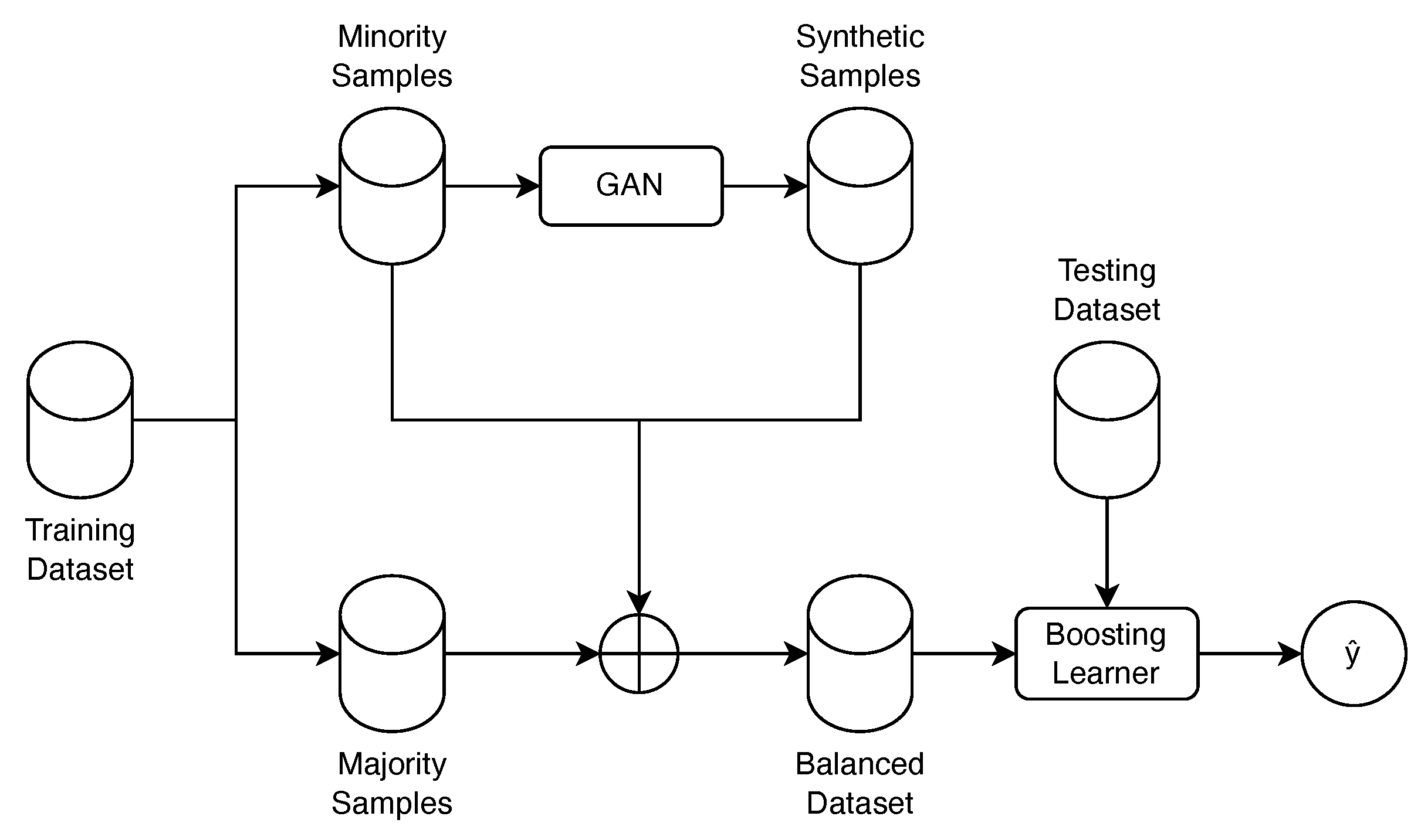
We propose an approach to combine GAN-based methods with boosting ensemble learning to handle the imbalance problem of software defects and improve the overall defect prediction. Our approach is a two-step approach as shown in Figure 1. In the first step, we use GAN-based methods to generate synthetic data from the minority class (i.e., defective modules). Then, we combine the generated synthetic data with the original data to produce a balanced dataset. In the second step, we employ a boosting ensemble on the balanced dataset to classify the modules in the software defects datasets. Our approach leverages the advantages of both GAN methods and boosting ensembles. GAN models have the ability to detect the overall data distribution and generate synthetic data that is very similar to the original data [5,6]. In addition, boosting ensemble has been proven to be suitable in handling imbalance problems by assigning a higher weight to the minority class [11,12]. Algorithm 2 outlines the algorithm of the proposed approach.

Algorithm 2 Algorithm of the proposed approach

Require: Dataset $D_n(x_1,c_1),\dots ,(x_n,c_n)$ Ensure: Imbalance classification model   1: Generate s synthetic samples   2: Create a new dataset $D_z$ of size z by combining the synthetic samples with the original samples, where z = $s+n$   3: Initialize samples weights $w_i=1/z,i=1,\dots ,z$   4: for $m\leftarrow 1$ to M do   5:  Train a weak learner $T_k^{\left(m\right)}\left(x\right)$ on Distribution $D_z$   6:  Obtain the weighted class probability estimates:      $p_k^{\left(m\right)}\left(x\right)=Pro{b}_w(c=k|x),k=1,\dots ,K$   7:  Set:      $h_k^{\left(m\right)}\left(x\right)\leftarrow (K-1)\left(log{p}_k^{\left(m\right)}\left(x\right)-\frac{1}{K}{\sum }_{k^{\prime }}log{p}_{k^{\prime }}^{\left(m\right)}\left(x\right)\right),k=1,\dots ,K$   8:  Set:      $w_i\leftarrow w_i·exp\left(-\frac{K-1}{K}{y}_i^{T}log{p}^{\left(m\right)}\left(x_i\right)\right),i=1,\dots ,z$   9:  Re-normalize $w_i$   10: end for   11: Output:      $C\left(x\right)=argmax{\sum }_{m=1}^M{h}_k^{\left(m\right)}\left(x\right)$

5. Empirical Study

This section describes the empirical study that we conducted to achieve our objectives. All experiments were conducted using Python programming languages. Stratified Shuffle Split was used to split the datasets into 80% and 20% for training and testing, respectively. All experiments were run ten times, and then we computed the average of these runs to get the final result.

5.1. Datasets Description

Many software defect datasets are available to the public. In this study, we utilized ten datasets from different projects to conduct our empirical study. These datasets have different sizes and imbalance ratios. Table 3 summarizes the characteristics of each defect dataset. NASA MDP datasets were published by [38]. These datasets contain static code metrics (i.e., Halstead, McCabe, and line of code metrics). Since these datasets contain some quality issues, such as missing values and duplicated samples, Shepperd et al. [39] processed these datasets and produced cleaner versions. Thus, we used the cleaned versions in our study.

Eclipse-2.0 is a publicly available dataset provided by [40]. It contains data from the open-source project ’Eclipse’ with different static code metrics, such as McCabe cyclomatic complexity and number of method calls. The Zxing dataset is collected by [41] and contains data from RELINK, which is an open-source project. This dataset contains different metrics categorized into Cyclomatic metrics (e.g., AvgCyclomati) and Line of Code metrics (e.g., CountLineCode). The Lucene-single version dataset [42] contains Chidamber and Kemerer (CK) metrics (e.g., depth of inheritance tree and number of children) and other Object-Oriented metrics (e.g., number of attributes and number of methods). Tomcat and prop-43 datasets [43] were collected from proprietary and open-source projects. These datasets contain different metrics suites, such as CK metrics and McCabe’s metrics.

Table 3. Datasets description.

Dataset	Number of Individual Features	Number of Samples	Number of Defective Samples	Imbalance Ratio
CM1 [39]	37	327	42	6.78
PC2 [39]	36	745	16	45.56
MC1 [39]	38	1988	46	42.21
MC2 [39]	39	125	44	1.84
JM1 [39]	21	7782	1672	3.65
Eclipse-2.0 [40]	31	6729	975	5.90
Tomcat [43]	20	1162	77	14.09
Prop-43 [43]	20	11,679	341	33.24
Zxing [41]	51	399	83	2.38
Lucene [42]	17	691	64	9.79

Table 3. Datasets description.

Dataset	Number of Individual Features	Number of Samples	Number of Defective Samples	Imbalance Ratio
CM1 [39]	37	327	42	6.78
PC2 [39]	36	745	16	45.56
MC1 [39]	38	1988	46	42.21
MC2 [39]	39	125	44	1.84
JM1 [39]	21	7782	1672	3.65
Eclipse-2.0 [40]	31	6729	975	5.90
Tomcat [43]	20	1162	77	14.09
Prop-43 [43]	20	11,679	341	33.24
Zxing [41]	51	399	83	2.38
Lucene [42]	17	691	64	9.79

5.2. Data Preprocessing

Data preprocessing is an essential task to prepare and transform the data into a suitable form for machine learning models. Handling missing values is one of the important preprocessing steps. Different methods were proposed to handle the missing values, such as mean imputation, median imputation, removing missing values, and nearest neighbor imputation. Mean imputation substitutes missing values with the mean of all known values of the column. It is one of the most commonly used techniques and has been shown to be efficient with supervised machine learning models [44]. Thus, in this study, we utilized the mean imputation to deal with the missing values.

Dealing with high-dimensional data is a challenging task before we build machine learning models. Feature selection can deal with this issue by selecting the most relevant features [45]. There are three main feature selection categories: filter, wrapper, and embedded methods. Filtering methods are faster than the other methods because they filter the attributes independently from the classification model. Filtering methods filter the attributes based on a specific metric such as chi-square, information gain, or gain ratio. Information gain calculates the dependency between independent attributes (features) and dependent attributes (target variable). It can be calculated as follows:

$$\mathrm{Information}\mathrm{Gain}\left(Y,X\right)=E\left(Y\right)-E\left(Y|X\right)$$

(5)

where:

• E(Y) is the entropy of the target variable (Y).
• H(Y|X) is the conditional entropy of Y given X.

However, feature selection using information gain suffers from bias towards features that have more distinct values. Thus, the gain ratio was proposed to decrease the bias in information gain by taking into account intrinsic information. The gain ratio is a normalized version of information gain. Equations (6) and (7) present the equations of gain ratio and intrinsic information, respectively.

$$\mathrm{Gain}\mathrm{ratio}\left(Y,X\right)=\frac{\mathrm{Information}\mathrm{Gain} (\mathrm{Y},\mathrm{X})}{\mathrm{Intrinsic}\mathrm{value} \left(\mathrm{X}\right)}$$

(6)

$$\mathrm{Instrinsic}\mathrm{value}\left(\mathrm{X}\right)=-\sum \frac{|S_i|}{S}\times lo{g}_2\frac{|S_i|}{S}$$

(7)

where:

• $\left|S\right|$ is the number of all values of the feature X.
• $|S_i|$ is the count of each distinct value of the feature X.

In this study, we utilized gain ratio to select the most relevant features which was used previously in the literature with ensemble learning in the field of software defect prediction [21].

5.3. Implementation Details

We used the scikit-learn library to implement AdaBoost, SMOTE, ROS, and RUS. For the implementation of GAN and CWGANGP, we used the ydata-synthetic library, which is an open-source library that provides implementations of different versions of GAN for tabular data. For GAN methods, ydata-synthetic uses MinMaxScaler to transform numerical data and One-hot encoding to transform categorical data. It also uses dense layers and a relu activation function for the generator and discriminator. Dropout was used after each dense layer in the discriminator. Lastly, the sigmoid activation function was utilized on the output of the GAN discriminator.

For CWGANGP methods, ydata-synthetic uses dense layers and leaky relu activation function in the generator and critic. Dropout was used after each dense layer in the critic. A synthetic data vault (SDV) package was used to implement CTGAN. The SDV package uses fully connected layers for the generator and critic of CTGAN. Relu activation function was used in the generator, and a mix of tanh and Gumbel softmax activation functions was used on the output. For the critic, the leaky relu activation function was used and dropout after each hidden layer.

5.4. GAN Hyperparameters Optimization

For hyperparameters optimization of GAN-based methods, we used Optuna [46], a hyperparameter optimization framework that provides different optimization algorithms, such as random search, grid search, and Bayesian optimization. In this study, we utilized the Bayesian optimization algorithm to find the best hyperparameters of GAN, CWGANGP, and CTGAN. We chose to examine the impact of learning rate, number of epochs, and batch size on the performance of GAN, CWGANGP, and CTGAN. Learning rate is the most important hyperparameter in neural networks [47]. It is the size of steps taken to reach a minimum loss. In other words, it controls how fast the model will learn. A number of epochs refers to the number of passes, i.e., each pass consists of one forward pass and one backward pass of the entire data through the network. Batch size controls the number of samples propagated in one pass.

Table 4. Hyperparameters range for optimization of GAN-based methods.

Hyperparameter	Range of Values
Number of epochs	100, 200, 300, 400, 500, 600, 700, 800, 900, 1000
Batch size	16, 32, 48, 64, 80, 94, 112, 128
Learning rate	0.0001, 0.0002, 0.0003, 0.0004, 0.0005

shows the range of hyperparameters that were used to optimize the GAN-based methods.

Cross-validation with three splits was used on the training set to find the optimal values of the hyperparameters. Then, we conducted the experiments using the optimal hyperparameters on the testing dataset. To investigate the impact of GAN hyperparameter optimization, we conducted the experiments using the default and optimized hyperparameter values. The default setting for epochs, batch size, and learning rate in ydata-synthetic (for GAN and CWGANGP) is 300, 128, and 0.0001, respectively, for CTGAN (in SDV), epochs, batch size, and learning rate are set to 300, 500, and 0.0002, respectively.

5.5. Combine GAN with Undersampling

One of the study objectives is to explore the effect of combining GAN-based methods with undersampling techniques to overcome the imbalance defect problem. We used RUS as our undersampling technique with optimized versions of the GAN-based methods. In our combination process, first, we calculated the difference between the number of majority-class and minority-class samples. Then, using GAN-based methods, we generated new minority-class synthetic samples that are equal to 50% of the calculated difference. RUS was then used to remove 50% of the calculated difference from the majority class samples.

5.6. Evaluation Metric

Evaluation metrics should be properly selected in order to accurately assess the performance of machine learning models. The most commonly used metric for evaluating classification models is accuracy. However, accuracy is not a reliable metric for evaluating imbalanced classification problems. Accuracy does not take into consideration the number of samples in each class. Instead, it considers the total number of predictions. Thus, it could yield a biased performance towards the majority class. Therefore, we selected a more reliable metric for imbalanced learning, which is Matthews Correlation Coefficient (MCC) [48]. MCC takes into consideration the number of samples in each class and yields a good result only if all confusion matrix elements (True positive (TP), True negative (TN), False positive (FP) and False negative (FN)) are good. Equation (8) presents the MCC equation.

$$MCC=\frac{TP\times TN-FP\times FN}{\sqrt{(TP+FP)\times (TP+FN)\times (TN+FP)\times (TN+FN)}}$$

(8)

5.7. Statistical Tests

We utilized the Wilcoxon effect size and Scott–Knott effect size difference as our statistical tests. We used Shapiro–Wilk test to verify the distribution of our study results, and results were not normally distributed. Thus, we used the Wilcoxon effect size [49] to answer the first and third research questions. Wilcoxon effect size is a non-parametric statistical test that can be used to determine the difference between two independent variables. The calculation of Wilcoxon effect size (r) is based on the Z-score and the number of samples (n), as shown in the following equation:

$$r=\frac{Z}{\sqrt{n}}$$

(9)

According to Cohen thresholds [50], the effect size (r) is interpreted as negligible, small, medium, or large. r is considered negligible if $r\le 0.1$, small if $0.1<r\le 0.3$, medium if $0.3<r\le 0.5$ and large if $0.5<r$. The Wilcoxon effect size was used to measure the difference between the performance of the default and optimized models and thus answer the first research question. In addition, the Wilcoxon effect size was used to estimate the impact of combining undersampling with GAN-based methods, and thereby answer the third research question.

In order to compare the performance of the traditional sampling techniques against GAN-based methods and answer the second research question, we utilized Scott–Knott ESD, which is a variant of the Scott–Knott test. This test uses a hierarchical clustering analysis to divide the methods into statistically different groups based on the mean value [51]. If the statistical difference between the methods is negligible, the methods will be merged into one group and given the same rank. Furthermore, if the difference between the methods is significant, then the methods will be placed into different groups.

6. Results and Discussion

In this section, we will discuss our empirical study results and answer the formulated research questions accordingly.

6.1. GAN Hyperparameter Optimization

In order to investigate the impact of hyperparameter optimization of GAN-based methods on defect prediction performance, we compared the performance of the GAN-based methods combined with boosting ensembles using the default against the optimized hyperparameters.

Table 5. MCC values of default and optimized GAN methods.

Dataset	Default			Optimized			Difference
	GAN	CWGANGP	CTGAN	GAN	CWGANGP	CTGAN	GAN	CWGANGP	CTGAN
CM1	0.05	0.12	0.07	0.10	0.07	0.11	0.05	−0.05	0.04
JM1	0.14	0.16	0.19	0.11	0.20	0.20	−0.03	0.03	0.00
MC1	0.18	0.04	0.15	0.24	0.28	0.18	0.06	0.24	0.03
MC2	0.08	0.02	0.14	0.20	0.20	0.25	0.12	0.18	0.10
PC2	0.11	−0.02	0.09	0.11	0.59	0.16	−0.01	0.61	0.08
Tomcat	0.22	0.23	0.22	0.24	0.27	0.33	0.02	0.04	0.11
Lucene	0.11	0.08	0.13	0.10	0.08	0.16	0.00	0.01	0.03
Eclipse-2.0	0.35	0.36	0.34	0.33	0.36	0.35	−0.02	0.00	0.01
Zxing	0.07	0.14	0.15	0.19	0.28	0.22	0.12	0.13	0.06
Prop-43	0.29	0.40	0.28	0.30	0.38	0.30	0.00	−0.02	0.03

presents the MCC values of the default and optimized GAN-based methods of the proposed approach on all defect datasets. The difference will be positive if optimizing the hyperparameters increases the defect prediction performance compared to the default values, and the negative difference has the opposite meaning. To quantify the difference between the performance of the default and optimized methods, we calculated the Wilcoxon effect size of the methods as shown in

Table 6. Wilcoxon effect size of the GAN methods.

Dataset	GAN	CWGANGP	CTGAN
CM1	Medium	Negligible	Small
JM1	Negligible	Large	Negligible
MC1	Small	Large	Small
MC2	Medium	Large	Small
PC2	Small	Large	Medium
Tomcat	Small	Medium	Large
Lucene	Negligible	Negligible	Small
Eclipse-2.0	Negligible	Negligible	Small
Zxing	Large	Large	Medium
Prop-43	Negligible	Negligible	Large
Total	4 Negligible, 3 Small, 2 Medium, and 1 Large	4 Negligible, 1 Medium, and 5 Large	1 Negligible, 5 Small, 2 Medium, and 2 Large

.

Empirical results demonstrated that GAN is slightly affected by hyperparameter optimization. Optimizing hyperparameters had a minor effect on 70% of the defect datasets, as shown in Table 6. This effect was found to be negative on 40% of the defect datasets. In other words, there is a slight reduction in MCC values of GAN on JM1, PC2, Lucene, and Eclipse-2.0 after performing the hyperparameters optimization process. Additionally, there was a positive moderate performance impact on the CM1 and MC2 defect datasets and a large positive impact on the Zxing defect dataset.

In the CWGANGP method, we observed that it was severely influenced by hyperparameter optimization. There was a large positive impact on 50% of the defect datasets and a medium impact on one defect dataset. In addition, there was a negligible impact on 40% of the defect datasets. This negligible impact was negative on CM1, Eclipse-2.0, and prop-43 defect datasets. Lastly, in the case of CTGAN methods, hyperparameter optimization yielded a positive performance impact on all defect datasets. It was slightly affected on 60% of the defect datasets; there was a negligible impact on JM1 and a small impact on CM1, MC1, MC2, Lucene, and Eclipse-2.0 datasets. Furthermore, it was highly impacted by hyperparameter optimization on 40% of the defect datasets, with a medium impact on PC2 and Zxing datasets and a large impact on Tomcat and Prop-43 datasets.

Clearly, the prediction performance of the optimized GAN-based models outperformed the default models on at least 60% of the defect datasets. Based on our empirical results, we can observe that GAN-based methods are sensitive to hyperparameter optimization. Thus, in the remaining experiments, we utilized the optimized models. We can summarize the answer of the first research question “RQ1. Will hyperparameters optimization of GAN-based methods yield enhanced defect prediction performance over default hyperparameters?”, as follows:

RQ1 answer. Empirical evidence demonstrated that hyperparameters optimization of GAN-based methods has a vital role in software defect prediction performance. The performance of the optimized models was superior over the default models on most of the defect datasets. The magnitude of the impact of hyperparameter optimization differs based on the GAN methods and defect datasets. Therefore, we recommend the optimization of GAN hyperparameters in imbalanced software defect prediction.

6.2. Comparison between Gan and Traditional Methods

To compare the performance of GAN-based methods against traditional methods, we used the Scott–Knott ESD statistical test. Figure 2 presents the Scott–Knott rankings of GAN-based methods and traditional methods on each defect dataset based on the MCC values. GAN was first-ranked on 20% of the defect datasets (CM1 and MC2) and second-ranked on 20% of the datasets (MC1 and Lucene). GAN outperformed SMOTE on 50% of the defect datasets, and also outperformed both ROS and RUS on 50% of the defect datasets. Furthermore, it achieved a comparable performance to ROS on 20% of the defect datasets and a comparable performance to RUS on 30% of the defect datasets.

CWGANGP method was the best-performing model on 50% of the defect datasets and was the second-ranked model on 40% of the defect datasets (CM1, JM1, Tomcat, and Eclipse-2.0). CWGANGP outperformed SMOTE on 50% of the defect datasets and achieved comparable performance to SMOTE on 40% of the defect datasets. In addition, it performed better than ROS on 70% of the defect datasets and had comparable performance to ROS on 20% of the defect datasets. Furthermore, it outperformed RUS on 60% of the defect datasets and attained a comparable performance to RUS on one defect dataset. We observed that the CWGANGP method outperformed all other methods on highly imbalanced datasets (MC1, PC2, and prop-43).

The CTGAN method was the first-ranked method on 50% of the defect datasets (CM1, JM1, Lucene, MC2, and Tomcat) and the second-ranked method on Eclipse-2.0, PC2 and Zxing datasets. CTGAN outperformed SMOTE on 80% of the defect datasets and performed better than ROS on 70% of the defect datasets while attaining comparable results to ROS on 20% of the defect datasets. Furthermore, CTGAN yielded a better performance than RUS on 70% of the defect datasets and achieved comparable performance to RUS on 30% of the defect datasets.

SMOTE, along with ROS, were the best-performing methods on one defect dataset only (Eclipse-2.0). Moreover, both SMOTE and ROS methods were the second-ranked methods on 50% and 40% of the defect datasets, respectively. RUS was first-ranked on CM1 and JM1 datasets due to the fact that the imbalance ratios of these datasets are small; thus, losing important information is less likely. On the other hand, we observe that RUS was the last ranked model on the highly imbalanced datasets (MC1, PC2, and prop-43) due to the information loss caused by the RUS method.

The Double Scott–Knott ESD statistical test was used to rank all methods across all defect datasets and provide a summary rank. Figure 3 presents the double Scott–Knott rankings of all methods. Clearly, we can observe that the CWGANGP and CTGAN methods were the best-performing methods. GAN and SMOTE methods achieved comparable performance and were the second-ranked methods. Overall, we can observe the GAN-based method’s ability to generate realistic and diverse data samples using the minority class distribution in comparison to other traditional methods. We can summarize the answer to the second research question, “RQ2. Will utilizing GAN-based methods yield enhanced defect prediction performance over traditional undersampling and oversampling techniques?”, as follows:

RQ2 answer. Empirical evidence proved the superiority of GAN-based methods in handling defect imbalance problems compared to traditional methods: SMOTE, ROS, and RUS. Among GAN methods, CWGANGP and CTGAN methods outperformed all other methods on most of the defect datasets. In addition, GAN outperformed ROS and RUS on most of the defect datasets and achieved a comparable performance to SMOTE.

6.3. Combining GAN-Based Methods with Undersampling

To explore the impact of undersampling with GAN-based methods, we compared the prediction performance of GAN-based methods with GAN-based methods combined with undersampling. Furthermore, the Wilcoxon effect size was utilized to quantify the difference between the performance of GAN-based methods against GAN-based methods combined with undersampling.

Table 7. MCC values of GAN-based methods with undersampling.

Dataset	GAN+U	CWGANGP+U	CTGAN+U
CM1	0.0635	0.0343	0.0249
JM1	0.1528	0.1817	0.2078
MC1	0.0248	0.4015	0.1747
MC2	0.1684	0.0487	0.0430
PC2	0.0770	0.4280	0.1051
Tomcat	0.2123	0.2145	0.2379
Lucene	0.0872	0.0841	0.1271
Eclipse-2.0	0.3599	0.3804	0.3454
Zxing	0.1630	0.1320	0.1908
Prop-43	0.3466	0.3249	0.3075

and

Table 8. Wilcoxon effect size of GAN-based methods with undersampling.

Dataset	GAN+U	CWGANGP+U	CTGAN+U
CM1	Negligible	Negligible	Negligible
JM1	Medium	Negligible	Medium
MC1	Negligible	Large	Negligible
MC2	Negligible	Negligible	Negligible
PC2	Negligible	Negligible	Negligible
Tomcat	Negligible	Negligible	Negligible
Lucene	Negligible	Negligible	Negligible
Eclipse-2.0	Large	Large	Negligible
Zxing	Negligible	Negligible	Negligible
Prop-43	Large	Negligible	Negligible
Total	7 Negligible, 1 Medium, 2 Large	8 Negligible, 2 Large	9 Negligible, 1 Medium

present the MCC values of GAN-based models combined with undersampling and the result of the Wilcoxon effect size, respectively.

As shown in Table 7 and Table 8, combining GAN with undersampling to overcome the imbalance problem caused a negligible negative impact on the prediction performance on 70% of the defect datasets. Eclipse-2.0, JM1, and prop-43 were positively affected by the combination of GAN and undersampling. On the contrary, combining CWGANGP with undersampling showed a negative effect on all defect datasets, except on MC1, Lucene, and Eclipse-2.0 datasets. There was a large positive impact of combining CWGANGP with undersampling on MC1 and Eclipse-2.0 datasets and a negligible positive impact on the Lucene dataset. It is worth noting that the prediction performance on all defect datasets was negatively affected by combining CTGAN with undersampling, except on JM1 and prop-43 datasets.

Integrating undersampling with GAN-based methods using the proposed approach caused a negative impact on 70% to 80% of the defect datasets. This can be linked to information loss, which is one of the drawbacks of undersampling. We can summarize the answer to the third research question, “RQ3. Will combining GAN-based methods with undersampling yield enhanced defect prediction performance?”, as follows:

RQ3 answer. On most defect datasets, combining GAN-based methods with undersampling using the proposed approach caused a degradation in the defect prediction performance. Undersampling can result in the removal of some important samples, which affects the overall prediction performance negatively. Thus, based on the empirical evidence, we do not recommend combining GAN-based methods with undersampling.

6.4. Threats to Validity

Using traditional evaluation metrics (e.g., accuracy, precision, and recall) to evaluate the performance on imbalanced datasets may lead to a biased performance. To mitigate this threat, we utilized MCC, which is a proper metric for imbalance classification problems. One threat to validity is related to the selection of the defect datasets. Our empirical results are based on the utilized defect datasets, which have different metrics (i.e., features). This may impact the validity of the results. To mitigate this threat, we selected different imbalanced defect datasets from different projects with different sizes and imbalance ratios. Moreover, these defect datasets are widely used and open sources, making our study results replicable and verifiable. GAN-based methods generate different samples of different qualities at each run of the experiment. To mitigate this threat, each experiment was repeated ten times, and the final result was the average of all runs. This step can validate the performance and avoid randomness of GAN outcomes.

7. Conclusions and Future Work

The main objective of this paper is to improve the performance of software defect prediction using a combination of GAN-based methods and boosting ensembles. We proposed combining GAN-based methods with boosting ensembles, where GAN-based methods are used to balance the datasets, and AdaBoost ensembles are employed to classify the modules into defective and non-defective modules. Furthermore, we used Optuna, the Bayesian model-based optimization algorithm, to find the optimal GAN hyperparameter values and explore the impact of the optimization process on the defect prediction performance. Paper outcomes can be summarized as follows: (1) GAN-based methods need hyperparameters optimization when used for imbalanced defect prediction. (2) GAN-based methods, namely CWGANGP and CTGAN, outperformed all traditional techniques: ROS, RUS, and SMOTE when used for imbalanced defect prediction. (3) GAN-based methods should be used to handle imbalance problems without combining it with undersampling techniques.

GAN-based methods proved to be a reliable sampling method to handle imbalanced software defect prediction due to their ability to generate new artificial and realistic samples from the minority class. However, GAN-based methods were found sensitive to their hyperparameters optimization. This work can be extended by exploring the performance of GAN-based methods with other ensemble learning algorithms (e.g., bagging). Moreover, other traditional and GAN-based methods could be included in future work to increase the generalizability of our study findings. Lastly, further studies might be conducted to evaluate the quality of the generated synthetic data using GAN-based methods and traditional methods.

References

- Huda, S.; Alyahya, S.; Ali, M.M.; Ahmad, S.; Abawajy, J.; Al-Dossari, H.; Yearwood, J. A framework for software defect prediction and metric selection. IEEE Access 2017, 6, 2844–2858. [Google Scholar] [CrossRef]
- Miraj, Z. Software Defect Severity Level Prediction Using Machine Learning Techniques. Ph.D. Thesis, Assam Science and Technology University (ASTU), Guwahati, India, 2021. [Google Scholar]
- Wahono, R.S.; Suryana, N. Combining particle swarm optimization based feature selection and bagging technique for software defect prediction. Int. J. Softw. Eng. Appl. 2013, 7, 153–166. [Google Scholar] [CrossRef]
- Tosun, A.; Bener, A.; Kale, R. Ai-based software defect predictors: Applications and benefits in a case study. In Proceedings of the Twenty-Second IAAI Conference, Atlanta, GA, USA, 11–15 July 2010. [Google Scholar]
- Goodfellow, I.; Pouget-Abadie, J.; Mirza, M.; Xu, B.; Warde-Farley, D.; Ozair, S.; Courville, A.; Bengio, Y. Generative Adversarial Nets. In Proceedings of the Advances in Neural Information Processing Systems, Montreal, QC, USA, 8–13 December 2014; Ghahramani, Z., Welling, M., Cortes, C., Lawrence, N., Weinberger, K., Eds.; Curran Associates, Inc.: New York, NY, USA, 2014; Volume 27. [Google Scholar]
- Engelmann, J.; Lessmann, S. Conditional Wasserstein GAN-based oversampling of tabular data for imbalanced learning. Expert Syst. Appl. 2021, 174, 114582. [Google Scholar] [CrossRef]
- Xu, L.; Skoularidou, M.; Cuesta-Infante, A.; Veeramachaneni, K. Modeling tabular data using conditional gan. Adv. Neural Inf. Process. Syst. 2019, 32. [Google Scholar]
- Chawla, N.V.; Bowyer, K.W.; Hall, L.O.; Kegelmeyer, W.P. SMOTE: Synthetic minority over-sampling technique. J. Artif. Intell. Res. 2002, 16, 321–357. [Google Scholar] [CrossRef]
- Zhou, Z.H. Ensemble Methods: Foundations and Algorithms; CRC Press: Boca Raton, FL, USA, 2012. [Google Scholar]
- Zhou, Z.H.; Zhou, Z.H. Ensemble Learning; Springer: Berlin/Heidelberg, Germany, 2021. [Google Scholar]
- Díez-Pastor, J.F.; Rodriguez, J.J.; Garcia-Osorio, C.; Kuncheva, L.I. Random balance: Ensembles of variable priors classifiers for imbalanced data. Knowl. Based Syst. 2015, 85, 96–111. [Google Scholar] [CrossRef]
- Thanathamathee, P.; Lursinsap, C. Handling imbalanced data sets with synthetic boundary data generation using bootstrap re-sampling and AdaBoost techniques. Pattern Recognit. Lett. 2013, 34, 1339–1347. [Google Scholar] [CrossRef]
- Hastie, T.; Rosset, S.; Zhu, J.; Zou, H. Multi-class adaboost. Stat. Interface 2009, 2, 349–360. [Google Scholar] [CrossRef]
- Chawla, N.V.; Lazarevic, A.; Hall, L.O.; Bowyer, K.W. SMOTEBoost: Improving prediction of the minority class in boosting. In Proceedings of the European Conference on Principles of Data Mining and Knowledge Discovery, Lyon, France, 13–16 September 2003; Springer: Berlin/Heidelberg, Germany, 2003; pp. 107–119. [Google Scholar]
- Seiffert, C.; Khoshgoftaar, T.M.; Van Hulse, J.; Napolitano, A. RUSBoost: Improving classification performance when training data is skewed. In Proceedings of the 2008 19th International Conference on Pattern Recognition, Tampa, FL, USA, 8–11 December 2008; IEEE: New York, NY, USA, 2008; pp. 1–4. [Google Scholar]
- Rodriguez, D.; Herraiz, I.; Harrison, R.; Dolado, J.; Riquelme, J.C. Preliminary comparison of techniques for dealing with imbalance in software defect prediction. In Proceedings of the 18th International Conference on Evaluation and Assessment in Software Engineering, London, UK, 13–14 May 2014; pp. 1–10. [Google Scholar]
- Li, J.; He, P.; Zhu, J.; Lyu, M.R. Software defect prediction via convolutional neural network. In Proceedings of the 2017 IEEE International Conference on Software Quality, Reliability and Security (QRS), Prague, Czech Republic, 25–29 July 2017; IEEE: New York, NY, USA, 2017; pp. 318–328. [Google Scholar]
- Pan, C.; Lu, M.; Xu, B.; Gao, H. An improved CNN model for within-project software defect prediction. Appl. Sci. 2019, 9, 2138. [Google Scholar] [CrossRef]
- Balogun, A.O.; Basri, S.; Said, J.A.; Adeyemo, V.E.; Imam, A.A.; Bajeh, A.O. Software defect prediction: Analysis of class imbalance and performance stability. J. Eng. Sci. Technol. 2019, 14, 3294–3308. [Google Scholar]
- Pradan, M.; Mizan, M.B.; Howlader, M.; Ripon, S. An Efficient Approach to Software Fault Prediction. In Proceedings of the International Conference on Communication, Computing and Electronics Systems, Chengdu, China, 26–26 April 2021; Springer: Singapore, 2021; pp. 221–237. [Google Scholar]
- Aljamaan, H.; Alazba, A. Software defect prediction using tree-based ensembles. In Proceedings of the 16th ACM International Conference on Predictive Models and Data Analytics in Software Engineering, Virtual, 8–9 November 2020; pp. 1–10. [Google Scholar]
- Alsaeedi, A.; Khan, M.Z. Software defect prediction using supervised machine learning and ensemble techniques: A comparative study. J. Softw. Eng. Appl. 2019, 12, 85–100. [Google Scholar] [CrossRef]
- Sun, Y.; Xu, L.; Li, Y.; Guo, L.; Ma, Z.; Wang, Y. Utilizing deep architecture networks of VAE in software fault prediction. In Proceedings of the 2018 IEEE Intl Conf on Parallel & Distributed Processing with Applications, Ubiquitous Computing & Communications, Big Data & Cloud Computing, Social Computing & Networking, Sustainable Computing & Communications (ISPA/IUCC/BDCloud/SocialCom/SustainCom), Melbourne, VIC, Australia, 11–13 December 2018; IEEE: New York, NY, USA, 2018; pp. 870–877. [Google Scholar]
- Kumar, P.S.; Venkatesan, R. Improving Software Defect Prediction using Generative Adversarial Networks. Int. J. Sci. Eng. Appl. 2020, 9, 117–120. [Google Scholar] [CrossRef]
- Chouhan, S.S.; Rathore, S.S. Generative Adversarial Networks-Based Imbalance Learning in Software Aging-Related Bug Prediction. IEEE Trans. Reliab. 2021, 70, 626–642. [Google Scholar] [CrossRef]
- Rathore, S.S.; Chouhan, S.S.; Jain, D.K.; Vachhani, A.G. Generative Oversampling Methods for Handling Imbalanced Data in Software Fault Prediction. IEEE Trans. Reliab. 2022, 71, 747–762. [Google Scholar] [CrossRef]
- Zheng, M.; Li, T.; Zhu, R.; Tang, Y.; Tang, M.; Lin, L.; Ma, Z. Conditional Wasserstein generative adversarial network-gradient penalty-based approach to alleviating imbalanced data classification. Inf. Sci. 2020, 512, 1009–1023. [Google Scholar] [CrossRef]
- Sun, Y.; Xu, L.; Guo, L.; Li, Y.; Wang, Y. A comparison study of vae and gan for software fault prediction. In Proceedings of the International Conference on Algorithms and Architectures for Parallel Processing, New York, NY, USA, 2–4 October 2020; Springer: Berlin/Heidelberg, Germany, 2020; pp. 82–96. [Google Scholar]
- Laradji, I.H.; Alshayeb, M.; Ghouti, L. Software defect prediction using ensemble learning on selected features. Inf. Softw. Technol. 2015, 58, 388–402. [Google Scholar] [CrossRef]
- Goyal, S.; Bhatia, P.K. Heterogeneous stacked ensemble classifier for software defect prediction. Multimed. Tools Appl. 2022, 81, 37033–37055. [Google Scholar] [CrossRef]
- Chen, L.; Fang, B.; Shang, Z.; Tang, Y. Tackling class overlap and imbalance problems in software defect prediction. Softw. Qual. J. 2018, 26, 97–125. [Google Scholar] [CrossRef]
- Huda, S.; Liu, K.; Abdelrazek, M.; Ibrahim, A.; Alyahya, S.; Al-Dossari, H.; Ahmad, S. An ensemble oversampling model for class imbalance problem in software defect prediction. IEEE Access 2018, 6, 24184–24195. [Google Scholar] [CrossRef]
- Fan, G.; Diao, X.; Yu, H.; Yang, K.; Chen, L. Software defect prediction via attention-based recurrent neural network. Sci. Program. 2019, 2019, 6230953. [Google Scholar] [CrossRef]
- Li, L.; Lessmann, S.; Baesens, B. Evaluating software defect prediction performance: An updated benchmarking study. arXiv 2019, arXiv:1901.01726. [Google Scholar] [CrossRef]
- Bahaweres, R.B.; Agustian, F.; Hermadi, I.; Suroso, A.I.; Arkeman, Y. Software Defect Prediction Using Neural Network Based SMOTE. In Proceedings of the 2020 7th International Conference on Electrical Engineering, Computer Sciences and Informatics (EECSI), Yogyakarta, Indonesia, 1–2 October 2020; IEEE: New York, NY, USA, 2020; pp. 71–76. [Google Scholar]
- Mehta, S.; Patnaik, K.S. Improved prediction of software defects using ensemble machine learning techniques. Neural Comput. Appl. 2021, 33, 10551–10562. [Google Scholar] [CrossRef]
- Shu, R.; Xia, T.; Williams, L.; Menzies, T. Dazzle: Using optimized generative adversarial networks to address security data class imbalance issue. In Proceedings of the 19th International Conference on Mining Software Repositories, Pittsburgh, PA, USA, 23–24 May 2022; pp. 144–155. [Google Scholar]
- Sayyad Shirabad, J.; Menzies, T. The PROMISE Repository of Software Engineering Databases; School of Information Technology and Engineering, University of Ottawa: Ottawa, ON, Canada, 2005. [Google Scholar]
- Shepperd, M.; Song, Q.; Sun, Z.; Mair, C. Data quality: Some comments on the nasa software defect datasets. IEEE Trans. Softw. Eng. 2013, 39, 1208–1215. [Google Scholar] [CrossRef]
- Zimmermann, T.; Premraj, R.; Zeller, A. Predicting defects for eclipse. In Proceedings of the Third International Workshop on Predictor Models in Software Engineering (PROMISE’07: ICSE Workshops 2007), Minneapolis, MN, USA, 20–26 May 2007; IEEE: New York, NY, USA, 2007; p. 9. [Google Scholar]
- Wu, R.; Zhang, H.; Kim, S.; Cheung, S.C. Relink: Recovering links between bugs and changes. In Proceedings of the 19th ACM SIGSOFT Symposium and the 13th European Conference on Foundations of Software Engineering, Szeged, Hungary, 5–9 September 2011; pp. 15–25. [Google Scholar]
- D’Ambros, M.; Lanza, M.; Robbes, R. An extensive comparison of bug prediction approaches. In Proceedings of the 2010 7th IEEE Working Conference on Mining Software Repositories (MSR 2010), Cape Town, South Africa, 2–3 May 2010; IEEE: New York, NY, USA, 2010; pp. 31–41. [Google Scholar]
- Jureczko, M.; Madeyski, L. Towards identifying software project clusters with regard to defect prediction. In Proceedings of the 6th International Conference on Predictive Models in Software Engineering, Timisoara, Romania, 12–13 September 2010; pp. 1–10. [Google Scholar]
- Mundfrom, D.J.; Whitcomb, A. Imputing Missing Values: The Effect on the Accuracy of Classification; ERIC: Washington, DC, USA, 1998.
- Cai, J.; Luo, J.; Wang, S.; Yang, S. Feature selection in machine learning: A new perspective. Neurocomputing 2018, 300, 70–79. [Google Scholar] [CrossRef]
- Akiba, T.; Sano, S.; Yanase, T.; Ohta, T.; Koyama, M. Optuna: A next-generation hyperparameter optimization framework. In Proceedings of the 25th ACM SIGKDD International Conference on Knowledge Discovery & Data Mining, New York, NY, USA, 4–8 August 2019; pp. 2623–2631. [Google Scholar]
- Goodfellow, I.; Bengio, Y.; Courville, A. Deep Learning; MIT Press: Cambridge, MA, USA, 2016. [Google Scholar]
- Chicco, D.; Jurman, G. The advantages of the Matthews correlation coefficient (MCC) over F1 score and accuracy in binary classification evaluation. BMC Genom. 2020, 21, 6. [Google Scholar] [CrossRef] [PubMed]
- Fritz, C.O.; Morris, P.E.; Richler, J.J. Effect size estimates: Current use, calculations, and interpretation. J. Exp. Psychol. Gen. 2012, 141, 2. [Google Scholar] [CrossRef] [PubMed]
- Cohen, J. A Power Primer; American Psychological Association: Washington, DC, USA, 2016. [Google Scholar]
- Scott, A.J.; Knott, M. A cluster analysis method for grouping means in the analysis of variance. Biometrics 1974, 30, 507–512. [Google Scholar] [CrossRef]