Deep Q Network Based on a Fractional Political–Smart Flower Optimization Algorithm for Real-World Object Recognition in Federated Learning

Abstract

An imperative application of artificial intelligence (AI) techniques is visual object detection, and the methods of visual object detection available currently need highly equipped datasets preserved in a centralized unit. This usually results in high transmission and large storage overheads. Federated learning (FL) is an eminent machine learning technique to overcome such limitations, and this enables users to train a model together by processing the data in the local devices. In each round, each local device performs processing independently and updates the weights to the global model, which is the server. After that, the weights are aggregated and updated to the local model. In this research, an innovative framework is designed for real-world object recognition in FL using a proposed Deep Q Network (DQN) based on a Fractional Political–Smart Flower Optimization Algorithm (FP-SFOA). In the training model, object detection is performed by employing SegNet, and this classifier is effectively tuned based on the Political–Smart Flower Optimization Algorithm (PSFOA). Moreover, object recognition is performed based on the DQN, and the biases of the classifier are finely optimized based on the FP-SFOA, which is a hybridization of the Fractional Calculus (FC) concept with a Political Optimizer (PO) and a Smart Flower Optimization Algorithm (SFOA). Finally, the aggregation at the global model is accomplished using the Conditional Autoregressive Value at Risk by Regression Quantiles (CAViaRs) model. The designed FP-SFOA obtained a maximum accuracy of 0.950, minimum loss function of 0.104, minimum MSE of 0.122, minimum RMSE of 0.035, minimum FPR of 0.140, maximum average precision of 0.909, and minimum communication cost of 0.078. The proposed model obtained the highest accuracy of 0.950, which is a 14.11%, 6.42%, 7.37%, and 5.68% improvement compared to the existing methods.

1. Introduction

FL is a distributed learning framework that can acquire a global or customized system from decentralized datasets on edge devices [1] and train the machine learning (ML) system [2] while preserving user data privacy. FL has the efficiency to restore large-scale computer vision (CV) applications, where centralized training cannot deal with diverse problems, like privacy concerns, data transfer, and maintenance expenses. More specifically, federated learning is a collaborative computing paradigm [3], and the main concept is to train the model by means of model aggregations instead of data aggregation, and local data remain at the local device. FL is a fascinating model that promotes end-to-end computer vision applications with image annotation and the training process moved to the edge while the model factors are transferred to the central cloud for aggregation purposes. Despite the tremendous growth in federated learning, current research still depends on existing public datasets that are specifically designed for ML. This results in significant constraints in model evaluations and benchmarks for FL and introduces real-world datasets produced from street cameras but manually selected and annotated. These datasets are a true illustration of real-time image data distributions [4] and, hence, are unbalanced. These images are carefully evaluated and assessed using elaborate statistics for the object distributions. YOLOv3 and Faster R-CNN are efficient algorithms integrated within federated learning models [1].

Object detection is the fundamental core of real-world applications like pedestrian detection, face detection, safety controls, and video assessment. With the recent advancements in deep learning (DL), object-detection algorithms have been highly utilized in the past few years. A conventional object-detection technique requires the gathering and centralization of large-scale annotated image data. Image annotation is very costly [5,6], specifically in fields where professional experts are needed. Moreover, centralizing such data requires the uploading of bulk information to a database, which experiences a high communication overhead. Ultimately, centralizing data may breach user privacy and data confidentiality, and individual data parties have zero control over how their data would be employed after centralization [7]. To handle the hurdle of data security and privacy in ML processes, numerous privacy-preserving ML techniques have been developed, like secure multi-party computing (MPC). MPC enables multiple parties to estimate a conventional parameter in a negligible way without disclosing their information either to each other or to a trusted third party. Nevertheless, conventional MPC protocols require a high communication overhead among parties, making them very difficult to consider in industrial fields. Differential privacy preserves user data by including noise, but it experiences a tradeoff between the risk of data leakage and model accuracy [8]. Owing to the unavailability of exploration in various tasks, the model performance of FL delivers superior results than centralized training [9]. Visual object detection involves significant AI models with large-scale applications in safety monitoring.

In recent years, visual-object detection training models have required the centralized storage of data. In these circumstances, individual users explicate visual information from locally owned cameras and upgrade such labeled data to the main server. Both the process of data storage and that of model training take place on the server [8]. For the past few years, object-detection advancements depending on deep neural networks have been widely employed in diverse fields, resulting in numerous advantages derived from the efficient feature extraction and illustration [10] capabilities of deep Convolutional Neural Networks (CNNs). The deep structure of a CNN yields efficient results in object-detection tasks [11,12], but the training cost of this network is high, which makes it very difficult for the model to perform well with sparse training data. Deep-CNN-based object-detection schemes are generally constructed in highly controlled environments, wherein the data are shared, centralized, and balanced, with the network having a high throughput. This is not possible in security, privacy, or regulatory domains. All the training data reside with the user, and no individual updates are preserved in the cloud [6]. A number of studies have been introduced on federated optimization and the minimization of the communication costs of transferring weights of deep networks. The accuracy of ensemble models was high, as they combined the prediction results from various models to obtain a final result [13,14,15,16]. Currently, the federated averaging algorithm has played a significant role in the training of classification models [17,18]. At the same time, it incurs a lot of problems in handling object detection, and it experiences more issues. One of the major hurdles is the statistical issue with highly non-IID and imbalanced data. Because of the complications of object-detection tasks and the huge weights of CNN models, the FedAvg algorithm is incapable of performing object-detection tasks.

The primary aim of this work is to construct a productive model for real-world object recognition in FL using the proposed FP-SFOA-DQN-FL. The entities involved in this designed model are nodes and servers. Here, local training is performed based on local data at every node, and the data are updated on the server. After that, model aggregation is carried out on the server, and the global model is downloaded at every node. Thereafter, updated training takes place based on the downloaded global model and local model at every epoch. In the training model, indoor images are taken into account as inputs, and they are subjected to a pre-processing stage, where the mechanism is carried out utilizing a bilateral filter to make the image desirable for further processing. Once the pre-processing is commenced, object detection is conducted by employing SegNet, and it is trained using PSFOA. The derived PSFOA is the combination of PO and SFOA. Following this process, features like ResNet, Shape Local Binary Texture (SLBT), gray level co-occurrence matrix (GLCM), speeded-up robust feature (SURF), oriented fast and rotated brief (ORB), and the Hierarchical Skeleton features are extracted. Finally, object recognition is performed utilizing DQN, in which parameters of the network are tuned optimally using designed FP-SFOA. The local updation and aggregation at the server are modified based on the CAViaR model.

Contributions of this research:

• FP-SFOA-DQN-FL for real-world object identification in FL: an efficacious model is developed for real-world object recognition in FL using FP-SFOA-DQN-FL.
• The object detection is conducted based on SegNet, and this classifier is optimally biased utilizing PSFOA.
• The object identification is accomplished utilizing DQN, and this network is optimally tuned based on modeled FP-SFOA.
• The FP-SFOA is derived by the consolidation of the FC concept with PO and SFOA.

The organization of this article is as follows: the literature review of former approaches associated with real-world object recognition in FL is explained in Section 2, along with its benefits and constraints that provoke the investigators to construct an effective framework. The designed model and its whole process associated with real world object recognition are enumerated in Section 3 and Section 4 discusses the outcomes of developed FP-SFOA-DQN-FL. Section 5 provides the satisfactory conclusion of this research along with its future scope.

2. Motivation

The pros and cons incurred by existing methods of the real object-recognition model in federated learning are reviewed along with its merits and issues that motivate research scholars to put forward effort to design an effectual framework for real object recognition in federated learning.

2.1. Literature Survey

Luo, J. et al. [1] designed a real-world image dataset to assess federated object-detection algorithms. This data distribution was non-IID and unbalanced, highlighting the properties of real-world federated learning conditions. Depending upon this dataset, two mainstream object-recognition techniques were introduced: YOLO and faster R-CNN. This method was considered a desirable benchmark for future federated learning research on how to mitigate the non-IID issue. The method was not able to augment the dataset. He, C. et al. [9] developed a federated learning library and benchmarking paradigm called FedCV to assess FL on three various computer vision tasks: image segmentation, image classification, and object detection. This method also provided non-IID benchmarking databases and different reference FL algorithms. However, non-IID databases generally deteriorated the model exactness to a certain degree in various processes. Also, increasing the effectiveness of federated learning is still a challenging problem. The method also lacks in exploring diverse tasks. Zhu, R. et al. [19] devised a Dilation RetinaNet Face Location (DRFL) Network that consists of an Enhanced Receptive Field Context (ERFC) system with the dilation convolution to minimize network parameters and found faces of various scales. Here, adaptation to embedded camera devices was accomplished using SRNet20 generated by a Neural Architecture Search (NAS). Because of security, SRNet20 was trained in federated learning. The DRFL network provided better performance, but the model was not capable of identifying the long-distance faces that were occluded. The implementation was not achieved using high-scale datasets that improve network detection. Liu, Y. et al. [8] modeled FedVision to assist the improvement in federated learning-powered computer vision applications. This advanced model effectively reduced the communication overhead. This method improved the operational efficiency but failed to obtain a sustainable mechanism.

Bommel, J.R. et al. [20] presented active learning that easily solved the unlabeled data and labeled it with an oracle. This article utilized various approaches using active learning to represent images locally and then exploit federated learning to train a global object-detection scheme. The developed model increased the precision level but decreased the communication costs. However, this model did not work well with non-homogeneous data. Yu, P. and Liu, Y. [21] introduced FedAVg to train models that provide the benefits of good privacy and security. Here, the weight divergence among various models trained with non-IID data was performed by exploiting KullbackLeibler Divergence (KLD). The newly developed FedAvg surpassed the effects of weight divergence influenced by non-IID and unbalanced data. In order to represent object detection, a Single Shot MultiBox Detector (SSD) was employed as the base model. This approach reduced the divergences, but the data found were ineffective due to the reduction in mapping. Hu, Z. et al. [22] designed a novel Inconsistency Capture module (ICM) to achieve the dynamic inconsistencies among successive frames of face forgery videos. The ICM comprised two parallel branches in which the first one took the entire successive frames as input to determine a global inconsistency illustration. The second one acquired the inter-frame difference of crucial areas to acquire the local instability. This model effectively worked on decentralized data. This model also ensured a high level of privacy and security. The method was incapable of enhancing the communication effectiveness of system factors to maximize the practicability of the FL paradigm. Tam, P. et al. [23] devised an adaptive model communication approach for edge federated learning using a Deep Q-learning algorithm to construct a self-learning agent communicating with network parameters and a software-defined, networking-based framework. The designed approach trained the learning model and weights for specific network states employing an epsilon-greedy approach. This method delivered maximum precision and effective QoS measures for dealing with future congestion scenarios. However, the method failed to compute the offloading decisions.

A review of existing methods is given in

Table 1. Review of literature survey.

Reference	Method	Advantages	Disadvantages
Luo, J. et al. [1]	Federated object-detection algorithms	It is able to mitigate non-IID issues.	It was not able to augment the dataset.
He, C. et al. [9]	FedCV	It is able to perform various computer vision tasks.	Increasing the effectiveness of federated learning was difficult.
Zhu, R. et al. [19]	DRFL	It provided better performance.	The implementation was not achieved using high-scale datasets.
Liu, Y. et al. [8]	FedVision	It reduced the communication overhead.	It failed to obtain sustainable mechanism.
Bommel, J.R. et al. [20]	Active learning	It increased the precision level.	It did not work well with non-homogeneous data.
Yu, P. and Liu, Y., [21]	FedAVg	It reduced the divergences.	It leads to reduction in mapping.
Hu, Z. et al. [22]	ICM	It effectively worked on decentralized data. It ensured high-level privacy and security.	It was incapable of enhancing the communication effectiveness of system factors.
Tam, P. et al. [23]	Adaptive model communication approach	It effectively deals with future congestion scenario.	It failed to compute the offloading decisions.

.

2.2. Major Issues

Some of the limitations experienced by traditional models of real-world object recognition in federated learning are listed below:

• Achieving real-time detection in crowded areas becomes a challenging issue in the existing models.
• Imbalanced data handling is another major issue in the existing object-detection models.
• Owing to network slicing in resolution image sensing, it was unable to update the needs of resource allocation, computation offloading resolutions, and service caching.
• The communication overhead of the conventional models is high.

3. Proposed FP-SFOA-DQN-FL for Real-World Object Recognition in FL

The foremost goal of this research is to predict real-world object recognition in federated learning using the proposed FP-SFOA-DQN-FL. The overall process will be explained as follows: initially, the dataset from [24] are fed as input to the device at the time, and the appropriate local training is achieved based on the local data at every node.

The architecture for a proposed model for real-world object recognition in FL is shown in Figure 1. In every node, the data are updated to the server, while model aggregation takes place at the server. Thereafter, the global model is downloaded at the nodes. Then, update training is carried out based on the downloaded global model and local model at every epoch. Here, object recognition is accomplished using the proposed FP-SFOA, which is a consolidation of the FC concept with PO and SFOA. The local updation and aggregation at the server will be modified based on the Conditional Autoregressive (CAViaR) [25].

3.1. Local Training Depending upon Local Data

This segment delineates the local training process depending on local data. In order to preserve the privacy of image data and to minimize the burden of the network, a predictor that is trained in a distributed way is preferred rather than transferring the original data to a central authority. In this module, local devices interact with a server continuously to learn the global model. At every epoch, a group of selected devices performs local training depending on local data and transmits the local updates to the server. After aggregating the updates at the server, it resends the global model to the devices. This process continues over the network till the specific criterion is satisfied [26].

3.1.1. Training at Every Node

For every time $t$, image data are trained on each device node. In addition, the object-recognition process is performed at the training model of each device, which is elaborately described in the following sections.

3.1.2. Training Model

The process of object recognition is performed at the training model of each device. The first step is to acquire the indoor images from a specific dataset field [24], and it is then pre-processed using a bilateral filter for the purpose of discarding the noises. The object-detection process is successfully accomplished through SegNet, which is trained using the designed PSFOA, and it is the combination of PO and SFOA. After detecting the objects, features, namely ResNet feature, SLBT, GLCM, SURF, ORB, and Hierarchical Skeleton, features are extracted at the feature-extraction phase. The refined feature vector is fed as an input to the object-recognition module, where the objects are clearly identified using DQN, and this network is tuned based on developed FP-SFOA. This modeled approach is obtained by the integration of the FC concept with PO and SFOA.

The pictorial representation of the object-recognition process performed in the training model is illustrated in Figure 2.

3.2. Data Acquisition

The process begins by acquiring the input image data from a specific database $O$ with $b$ count of total image samples, and it is expressed as

$$O=\left\{I_1,\hspace{0.17em}{I}_2,\hspace{0.17em}{I}_3,\dots ,I_a,\dots ,I_b\right\}$$

(1)

Here, $I_a$ represents the $a\mathrm{th}$ image available at dataset $O$, and the overall amount of training samples in the database is denoted as $I_b$.

3.3. Pre-Processing Utilizing Bilateral Filter

The image, $I_a$, is subjected to the pre-processing phase to eliminate the calamities and noises that exist in the image. The bilateral filter [27] substitutes the center pixel of a block with an estimated pixel, which is a weighted average that considers the spatial as well as tonal distances among pairs of pixels in the block. The weighted average considers the information of the same pixels with the same tone. The benefit of a bilateral filter is that it efficiently eliminates the noise and preserves the edge information. The bilateral filter is expressed by

$$\Re \hspace{0.17em}{\left[P\right]}_x=\frac{1}{w_x}\hspace{0.17em}{\displaystyle \sum _{y\in {\rm M}}^{}G{a}_{{\sigma }_{SD}}\hspace{0.17em}\left(‖x-y‖\right)\hspace{0.17em}G{a}_{{\sigma }_{TD}}\hspace{0.17em}\left(\left|P_x-P_y\right|\right)\hspace{0.17em}{P}_y}$$

(2)

Here, $\Re {\left[P\right]}_x$ signifies the restored measure of pixel $x$, and the standard deviation of spatial distance and tonal distance of neighboring cells are specified as ${\sigma }_{SD}$ and ${\sigma }_{TD}$, respectively. $Ga$ shows the Gaussian parameter, and P sub x and P sub y signify the pixel contrasts of pixels and. Moreover, the group of neighboring pixels fixed at $x$ is represented as $M$ and, and the total weights within the block are depicted as $w_x$. Finally, the pre-processed outcome is expressed as $B_a$.

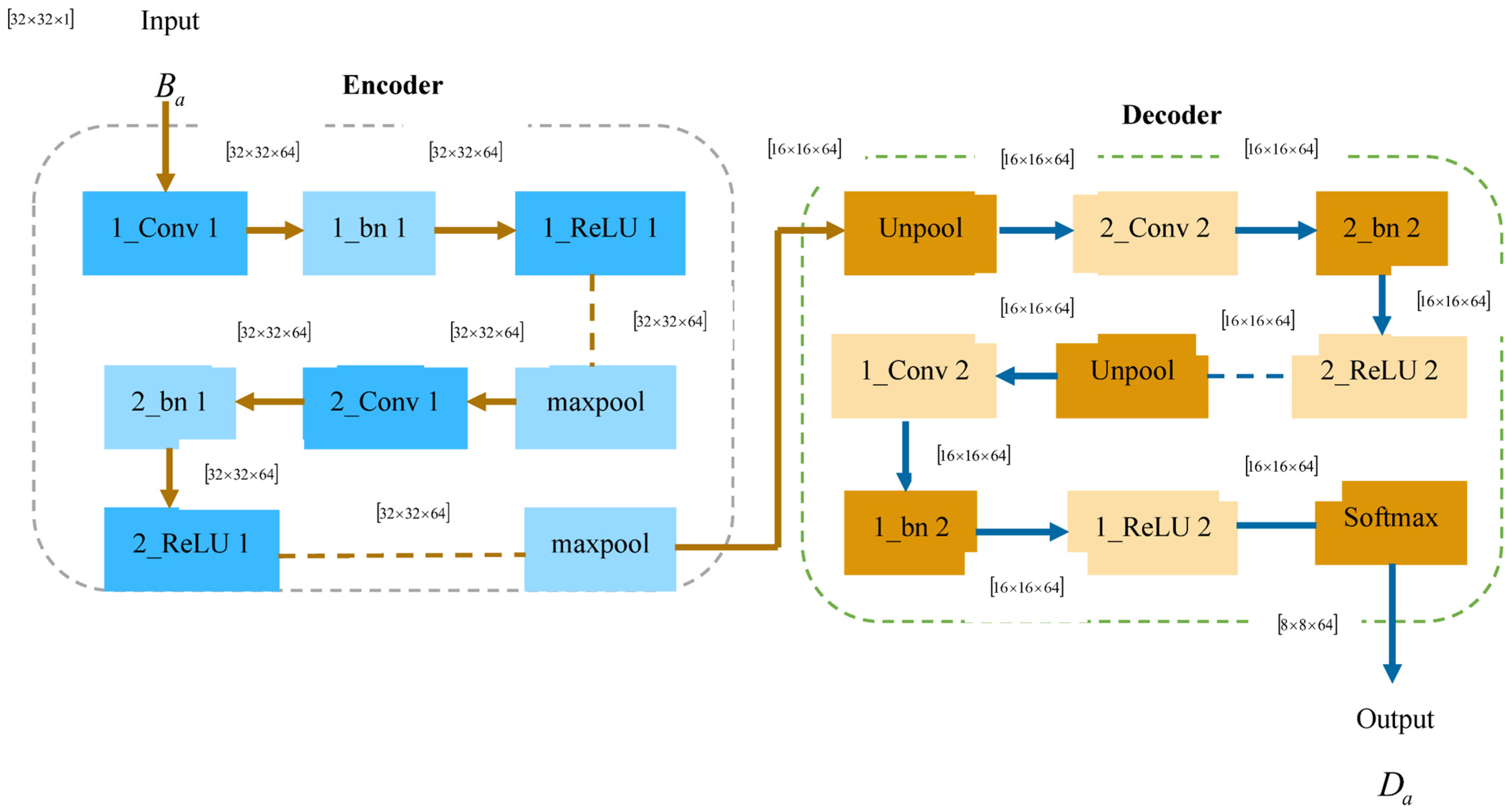
3.4. Object Detection Using SegNet

The pre-processed outcome $B_a$ is injected into the object-detection stage, where objects are accurately detected by employing SegNet. It is specifically developed to be an effective structure for pixel-wise semantic segmentation. The spatial differences between diverse classes are very comprehensible. Also, the SegNet used few trainable parameters, so it is more efficient in terms of computation time, accuracy, and memory.

• Structural diagram of SegNet

SegNet [28] consists of an encoder and decoder network, succeeding with a pixel-wise classification layer. The encoder includes 13 convolutional layers, which are particularly designed for object classification. The training process will be initialized from weights tuned for categorization on huge databases. The fully connected layers are eliminated to extract the higher-resolution feature maps, and it also minimizes the quantity of SegNet parameters. Each encoder has its respective decoder, so the decoder network consists of 13 layers. Finally, the decoder result is subjected to a softmax classifier to generate class probabilities for individual pixels. The layers in the SegNet are elaborated as follows:

• Encoder network

This network applies convolution operation with a filter bank to generate a pool of feature maps. After that, the feature maps undergo a batch-normalized operation, and an element-wise function is performed utilizing a Rectified Linear Unit (ReLU). Following this, a max-pooling operation and non-overlapping window are carried out, and the final outcome is sub-sampled utilizing a parameter of 2. Sub-sampling generates a huge input image context within the feature map. However, numerous max-pooling and sub-sampling layers result in high translation invariance for effective classification. This lossy image illustration is not suitable for the segmentation process. In order to address this gap, it is imperative to grasp and preserve the boundary data in the encoder feature maps.

2.

Decoder network

In this network, it up-samples its feature maps employing the retained max-pooling indices from respective encoder feature maps. During this phase, sparse feature maps are generated. Such feature maps are again convolved with a trained decoder filter bank to generate dense feature maps. Then, the feature maps are processed using a batch-normalization step. It is notable that the decoder, with respect to its first encoder, generates a multi-channel feature map, even if the encoder input has three channels.

3.

Softmax classifier

The result of the final decoder, which is a high-dimension feature representation, is subjected as an input to the trainable soft-max classifier. The outcome of the soft-max classifier is a $K$ channel image of probabilities, which specifies the count of classes. The detected result obtained through SegNet is denoted as $D_a$. Figure 3 portrays the structural diagram of SegNet.

ii.

Training of SegNet using proposed PSFOA

In order to attain an accurate detected object result, it is significant to train the SegNet with an efficient hybrid optimization at every epoch until the satisfied result is obtained. Here, a hybrid algorithm named PSFOA is employed, which is designed by the combination of PO with SFOA. SFOA [29] is inspired by the immature sunflowers that generate heliotropic movements. Here, two growth strategies are managed on the heliotropic motions of baby sunflowers. The initial process is the sun-tracking occurrence, which is influenced by a growth hormone known as Auxin. On the other hand, the second strategy is the biological clock. Moreover, this technique has been introduced in two stages, namely, sunny and rainy or cloudy phases. PO [30] is a socially inspired metaheuristic algorithm that is inspired by the multi-phased process of politics. This algorithm allocates a double role by partitioning the population into political parties and constituencies. Integrating these two algorithms can provide better detection results with high convergence speed.

• Smart Flower position encoding

The purpose of position encoding is to determine the supreme solution that solves the optimization problem in an efficient way. Here, the population in a $\mathrm{G}$-dimensional area is solved, such that $G=\left[1 X \eta \right]$, and $\eta$ is the learning factor of SegNet.

• Objective function

The prime objective of the fitness factor is to evaluate the finest solution using the expression that defines the change in variation between the targeted output and the output of SegNet.

$$\Im =\frac{1}{b}\hspace{0.17em}{\displaystyle \sum _{a=1}^b\left[{\tau }_a-D_a\right]{\hspace{0.17em}}^2}$$

(3)

where $b$ symbolizes the overall quantity of image samples, ${\tau }_a$ is the targeted result, and the output of SegNet is indicated as $D_a$.

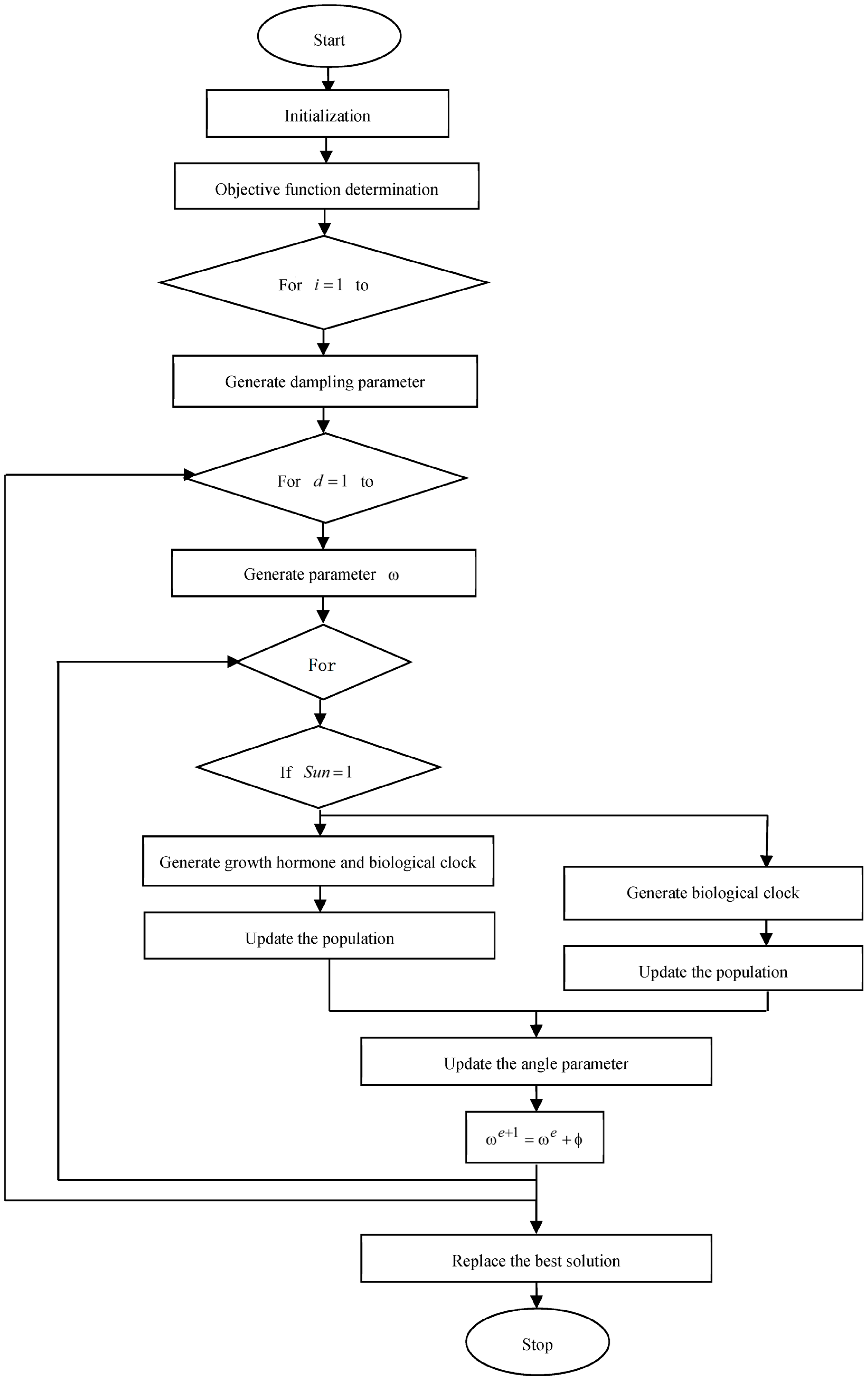
• Algorithmic steps of proposed PSFOA

The algorithmic procedures included in the devised PSFOA are enumerated as follows:

• Step 1. Initialization of Sunflower population

The population of sunflowers is initialized in a G-dimensional area, and in this algorithm, the updating mechanism of search agents can be accomplished depending on the growth of baby sunflowers. Here, individual baby sunflowers are taken into account to have a stem length in a $\mathrm{G}$-dimensional search area. Thus, the group of immature sunflowers can be expressed in the form of a matrix as

$$S=\left[\begin{array}{l}{S}_{1,1}\hspace{0.17em}\hspace{0.17em}\hspace{0.17em}\hspace{0.17em}\hspace{0.17em}\hspace{0.17em}{S}_{1,2}\cdots \cdots S_{1,G}\\ S_{2,1}\hspace{0.17em}\hspace{0.17em}\hspace{0.17em}\hspace{0.17em}\hspace{0.17em}\hspace{0.17em}{S}_{2,2}\dots \dots S_{2,G}\\ \hspace{0.17em}⋮\hspace{0.17em}\hspace{0.17em}\hspace{0.17em}\hspace{0.17em}\hspace{0.17em}\hspace{0.17em}\hspace{0.17em}\hspace{0.17em}\hspace{0.17em}\hspace{0.17em}⋮\hspace{0.17em}\hspace{0.17em}\hspace{0.17em}\hspace{0.17em}\hspace{0.17em}\hspace{0.17em}\hspace{0.17em}\hspace{0.17em}\hspace{0.17em}⋮\\ S_{o,1}\hspace{0.17em}\hspace{0.17em}\hspace{0.17em}\hspace{0.17em}\hspace{0.17em}\hspace{0.17em}{S}_{o,2}\dots \dots S_{o,G}\end{array}\right]$$

(4)

Here, $o$ refers to the overall count of baby sunflowers, and the quantity of variables in the search area is indicated as $G$.

• Step 2. Determine objective function

The stem length of an individual sunflower delivers the optimal solution to an optimization problem. Each sunflower has a fitness parameter in accordance with the measure of the fitness value of the optimization issue that illustrates the long sunflower’s stem. The objective function is evaluated using Equation (3).

• Step 3. Evaluate the first mode

New solutions are generated depending upon an internal process that enables sunflowers to get ready to fulfill their development level during the latest day in the decision area. This internal mechanism purely depends upon solar tracking during the daytime and the biological clock during night-time. The development process of the baby sunflower is introduced in two stages: sunny and cloudy modes. The factor “Sun” is employed to represent sunny or cloudy modes. If it is set to 1, then the day is said to be sunny, and if it is set to 0, then the day is said to be cloudy. The mathematical expression of the sunny mode is given by

$$X_{new,\hspace{0.17em}S}^{i+1}=\left\{\begin{array}{l}{X}_{old,\hspace{0.17em}S}^i+c\times \mathit{Sin}\hspace{0.17em}\left(\omega \right)\times \hspace{0.17em}\left[\chi \times X_{best,\hspace{0.17em}S}^i-X_{old,\hspace{0.17em}S}^i\right],\hspace{0.17em}hours\hspace{0.17em}\hspace{0.17em}day\le 24\\ X_{old,\hspace{0.17em}S}^i+c\times \mathit{Sin}\hspace{0.17em}\left(\omega \right)\times \left[X_{best,\hspace{0.17em}S}^i-X_{old,\hspace{0.17em}S}^i\right],\hspace{0.17em}\hspace{0.17em}\hspace{0.17em}\hspace{0.17em}\hspace{0.17em}\hspace{0.17em}\hspace{0.17em}\hspace{0.17em}\hspace{0.17em}Otherwise\end{array}\right.$$

(5)

Here, $X_{\mathit{new}, s}^i$ shows the $S\mathrm{th}$ component of the current optimal length of the sunflower’s stem at the $i\mathrm{th}$ iteration. Moreover, the Sine parameter defines heliotropic mechanism of the immature sunflowers, and $\omega$ represents the angle. Moreover, Auxin$\left(x\right)$ serves a significant part in sunflower as well as stem growth. It is highly responsible for variation in the natural motion of sunflowers, and x signifies growth hormone, which is in an active mode during normal hours of the day.

• Step 4. Generate damping parameter

In SFOA, the factor $c$ is the damping parameter. It is employed to initiate the termination of sunflower’s stem growth, and it is eventually decreased during every epoch using the below expression

$$c=c_{\max }-i\times \frac{\left(c_{\max }-c_{\min }\right)}{i_{\max }}$$

(6)

Here, $C_{max}$ and $C_{min}$ represent the maxima and minima measures of the damping factor, respectively. In addition, the latest iteration and the maximum count of iterations are, respectively, specified as $i$ and $i_{max}$.

• Step 5. Generate the Hours’ day parameter

The baby sunflowers managed their heliotropic growth based on the biotic clock, which is described as the period to execute one turn of 24 h day/night. If the time period increases, the immature sunflowers have a minimal capability to move forward and backward on a regular basis. In this algorithm, the hours’ day factor offers an uneven hour that is chosen within the limit of $\left[0, 100\right]$.

• Step 6. Update the solution

As mentioned earlier, immature sunflowers grow with respect to a mechanism known as heliotropism, which is proved to not be controlled only by direct sunlight but also by its biological clock. This movement rate is found to be minimal during rainy or cloudy days. This expression is mathematically formulated as follows:

$$X_{new,\hspace{0.17em}S}^{i+1}=X_{old,\hspace{0.17em}S}^i+c\times \mathit{Sin}\hspace{0.17em}\left(\omega \right)\ast \hspace{0.17em}\left[X_{best,\hspace{0.17em}S}^i-X_{old,\hspace{0.17em}S}^i\right]$$

(7)

$$X_{new,\hspace{0.17em}S}^{i+1}=X_{old,\hspace{0.17em}S}^i\hspace{0.17em}\left(1-c\times \mathit{Sin}\hspace{0.17em}\left(\omega \right)\right)+c\times \mathit{Sin}\hspace{0.17em}\left(\omega \right)\hspace{0.17em}\left[X_{best,\hspace{0.17em}S}^i\right]$$

(8)

The standard expression for PO is stated as follows:

$$\begin{array}{l}{M}_{g,\hspace{0.17em}k}^h\left(j+1\right)=M_{g,\hspace{0.17em}k}^h\left(j-1\right)+R\hspace{0.17em}\left(M_{g,\hspace{0.17em}k}^h\hspace{0.17em}\left(j\right)-M_{g,\hspace{0.17em}k}^h\hspace{0.17em}\left(j-1\right)\right)\hspace{0.17em}\hspace{0.17em}\hspace{0.17em}if\hspace{0.17em}\hspace{0.17em}{M}_{g,\hspace{0.17em}k}^h\hspace{0.17em}\left(j-1\right)\le z^{\ast }\le \hspace{0.17em}{M}_{g,\hspace{0.17em}k}^h\left(j\right)\hspace{0.17em}\hspace{0.17em}or\\ \hspace{0.17em}\hspace{0.17em}\hspace{0.17em}\hspace{0.17em}\hspace{0.17em}\hspace{0.17em}\hspace{0.17em}\hspace{0.17em}\hspace{0.17em}\hspace{0.17em}\hspace{0.17em}\hspace{0.17em}\hspace{0.17em}\hspace{0.17em}\hspace{0.17em}\hspace{0.17em}\hspace{0.17em}\hspace{0.17em}\hspace{0.17em}\hspace{0.17em}\hspace{0.17em}\hspace{0.17em}\hspace{0.17em}\hspace{0.17em}\hspace{0.17em}\hspace{0.17em}\hspace{0.17em}\hspace{0.17em}\hspace{0.17em}\hspace{0.17em}\hspace{0.17em}\hspace{0.17em}\hspace{0.17em}\hspace{0.17em}\hspace{0.17em}\hspace{0.17em}\hspace{0.17em}\hspace{0.17em}\hspace{0.17em}\hspace{0.17em}\hspace{0.17em}\hspace{0.17em}\hspace{0.17em}\hspace{0.17em}\hspace{0.17em}\hspace{0.17em}\hspace{0.17em}\hspace{0.17em}\hspace{0.17em}\hspace{0.17em}\hspace{0.17em}\hspace{0.17em}\hspace{0.17em}\hspace{0.17em}\hspace{0.17em}\hspace{0.17em}\hspace{0.17em}\hspace{0.17em}\hspace{0.17em}\hspace{0.17em}\hspace{0.17em}\hspace{0.17em}\hspace{0.17em}\hspace{0.17em}\hspace{0.17em}\hspace{0.17em}\hspace{0.17em}\hspace{0.17em}\hspace{0.17em}\hspace{0.17em}{M}_{g,\hspace{0.17em}k}^h\left(j-1\right)\ge z^{\ast }\ge M_{g,\hspace{0.17em}k}^h\left(j\right)\end{array}$$

(9)

Let us assume

$$M_{g,\hspace{0.17em}k}^h\left(j+1\right)=X_{new,\hspace{0.17em}S}^{i+1}$$

(10)

$$M_{g,\hspace{0.17em}k}^h\left(j-1\right)=X_S^{i-1}$$

(11)

$$M_{g,\hspace{0.17em}k}^h\left(j\right)=X_{old,\hspace{0.17em}S}^i$$

(12)

Then, the above expression becomes

$$X_{new,\hspace{0.17em}S}^{i+1}=X_S^{i-1}+R\hspace{0.17em}\left(X_{old,\hspace{0.17em}S}^i-X_S^{i-1}\right)\hspace{0.17em}\hspace{0.17em}$$

(13)

$$X_{old,\hspace{0.17em}S}^i\hspace{0.17em}=\frac{X_{new,\hspace{0.17em}S}^{i+1}+X_S^{i-1}\left(R-1\right)\hspace{0.17em}}{R}\hspace{0.17em}$$

(14)

Substituting Equation (14) in Equation (8), the equation becomes

$$X_{new,\hspace{0.17em}S}^{i+1}=\left(\frac{X_{new,\hspace{0.17em}S}^{i+1}+X_S^{i-1}\left(R-1\right)\hspace{0.17em}}{R}\right)\hspace{0.17em}\left(1-c\times \mathit{Sin}\hspace{0.17em}\left(\omega \right)\right)+c\times \mathit{Sin}\hspace{0.17em}\left(\omega \right)\hspace{0.17em}\left[X_{best,\hspace{0.17em}S}^i\right]$$

(15)

$$X_{new,\hspace{0.17em}S}^{i+1}-\frac{X_{new,\hspace{0.17em}S}^{i+1}}{R}\hspace{0.17em}\left(1-c\times \mathit{Sin}\hspace{0.17em}\left(\omega \right)\right)=\left(\frac{X_S^{i-1}\left(R-1\right)\hspace{0.17em}}{R}\right)\hspace{0.17em}\left(1-c\times \mathit{Sin}\hspace{0.17em}\left(\omega \right)\right)+c\times \mathit{Sin}\hspace{0.17em}\left(\omega \right)\hspace{0.17em}\left[X_{best,\hspace{0.17em}S}^i\right]$$

(16)

$$X_{new,\hspace{0.17em}S}^{i+1}\hspace{0.17em}\left[\frac{R-1+c\times \mathit{Sin}\hspace{0.17em}\left(\omega \right)}{R}\right]=\frac{X_S^{i-1}\hspace{0.17em}\left(R-1\right)\hspace{0.17em}\left(1-c\times \mathit{Sin}\hspace{0.17em}\left(\omega \right)\right)+R.c\times \mathit{Sin}\hspace{0.17em}\left(\omega \right)\hspace{0.17em}\left(X_{best,\hspace{0.17em}S}^i\right)}{R}$$

(17)

The updated solution of PSFOA is expressed as

$$X_{new,\hspace{0.17em}S}^{i+1}\hspace{0.17em}=\frac{X_S^{i-1}\hspace{0.17em}\left(R-1\right)\hspace{0.17em}\left(1-c\times \mathit{Sin}\hspace{0.17em}\left(\omega \right)\right)+R.c\times \mathit{Sin}\hspace{0.17em}\left(\omega \right)\hspace{0.17em}\left(X_{best,\hspace{0.17em}S}^i\right)}{R-1+c\times \mathit{Sin}\hspace{0.17em}\left(\omega \right)}$$

(18)

where $X_{\mathit{best},S}^i$ represents the $S\mathrm{th}$ component of the current supreme length of the sunflower’s stem at the $i\mathrm{th}$ iteration, and the damping factor is denoted as $c$. The mamum number of iterations is signified as $i_{\max }$, and the $S\mathrm{th}$ component of the length of the sunflower stem at the $\left(i-1\right)\mathrm{th}$ iteration is implied as $X_S^{i-1}$.

• Step 7. Termination

The process is iterated over and over till it satisfies the optimal solution. The pseudo-code of the proposed PSFOA is elucidated in Algorithm 1.

Algorithm 1 Pseudo-code of devised PSFOA

1 Input: Population size $0$, maximum count of iterations $({\mathrm{i}}_{\max })$, Number of decision variables $\left(\mathrm{G}\right)$, Sun parameter $\left(\mathrm{Sun}\right)$ 2 Output: ${\mathrm{X}}_{\mathrm{new}, \mathrm{S}}$ 3 Begin 4     Initialized the population 5     Evaluate fitness function utilizing Equation (3) 6 for $i=1$ to ${\mathrm{i}}_{\max }$ 7     Generate damping parameter $\mathrm{c}$ using Equation (6) 8 for $d=1$ to $0$ 9 Generate parameter $\mathsf{\omega }$ 10 for $e=1$ to $\mathrm{G}$ 11 if $Sun=1$ 12      Generate the growth hormone $\left(\mathrm{X}\right)$ and biological clock $\left({\mathrm{Hours}}^{\prime }day\right)$ 13 Update the population using Equation (5) 14 Else 15      Generate $\left({\mathrm{Hours}}^{\prime }day\right)$ parameter 16 Update the population using Equation (18) 17 end if 18 Upgrade the angle parameter $\varphi$ 19 ${\mathsf{\omega }}^{\mathrm{e}+1}={\mathsf{\omega }}^{\mathrm{e}}+\varphi$ 20 end for $\mathrm{e}$ 21 end for $\mathrm{d}$ 22      Replace ${\mathrm{X}}_{\mathrm{best}}$ by ${\mathrm{X}}_{\mathrm{new}, \mathrm{S}}$ 23 end for $\mathrm{i}$ 24 Return best solution 25 Terminate

The flowchart of the proposed PSFOA is shown in Figure 4.

3.5. Feature Extraction

The extraction of features is the most significant phase performed to extract the relevant features for future processing of object recognition. More appropriate features being extracted results in accurate object-recognition performance. Here, the features extracted at this step are described as follows:

Regarding the detected result ${\mathrm{D}}_{\mathrm{a}}$ of the object-detection process, the features are extracted.

• Shape Local Binary Texture (SLBT)

The SLBT feature [31] is an integration of shape and texture information. SLBT is similar to that of the active appearance model (AAM), and it considers LBP texture features rather than intensity measures. In AAM, direct intensity values from shape-free patches are employed for texture modeling. However, SLBT performs LBP over a shape-free patch to obtain illumination and unchanged noise features. LBP feature extraction is fast and simple.

Consider a $3\times 3$ window with a center pixel, where its intensity measure is represented as $l_c,$ and its local texture is represented as

$$Pix=pix\hspace{0.17em}\left(l_J\right)$$

(19)

Here, $l_J$ is associated with the grey measures of eight adjacent pixels in which $\left(J=0, 1, 2, 3, \dots ,7\right)$. These adjacent pixels are threshold with the middle value $l_c$ as $pix\left(Aa\left(l_0-l_{\mathrm{c}}\right),. . . , Aa \left(l_7-l_c\right)\right)$, and the function $Aa\left(N\right)$ is expressed as

$$Aa\hspace{0.17em}\left(N\right)=\left\{\begin{array}{l}1,\hspace{0.17em}\hspace{0.17em}\hspace{0.17em}\hspace{0.17em}N>0\\ 0,\hspace{0.17em}\hspace{0.17em}\hspace{0.17em}N\le 0\end{array}\right.$$

(20)

$$LBP={\displaystyle \sum _{J=0}^{7}Aa\hspace{0.17em}\left(l_J-l_C\right)\hspace{0.17em}{2}^J}$$

(21)

The LBP pattern at the middle pixel $l_c$ is achieved using the above equation, and the image result obtained from SLBT is denoted as $V_1$.

ii.

Speeded-Up Robust Feature (SURF);

SURF [32] is a local feature descriptor that is highly employed for functions like classification, object recognition, and 3D reconstruction. The identifier determines the interest points highlighted in the image, whereas the descriptor explains the features of interest points. Such features are invariable to shifting, rotation, and scaling. The SURF feature result $V_2$ is defined as follows:

$$V_2\hspace{0.17em}\left(\aleph ,\hspace{0.17em}\delta \right)=\left\{\begin{array}{l}{\mathrm{H}}_{uu}\hspace{0.17em}\left(\aleph ,\hspace{0.17em}\delta \right)\hspace{0.17em}\hspace{0.17em}\hspace{0.17em}\hspace{0.17em}\hspace{0.17em}\hspace{0.17em}\hspace{0.17em}\hspace{0.17em}\hspace{0.17em}\hspace{0.17em}\hspace{0.17em}\hspace{0.17em}{\mathrm{H}}_{uv}\hspace{0.17em}\left(\aleph ,\hspace{0.17em}\delta \right)\\ {\mathrm{H}}_{uv}\hspace{0.17em}\left(\aleph ,\hspace{0.17em}\delta \right)\hspace{0.17em}\hspace{0.17em}\hspace{0.17em}\hspace{0.17em}\hspace{0.17em}\hspace{0.17em}\hspace{0.17em}\hspace{0.17em}\hspace{0.17em}\hspace{0.17em}\hspace{0.17em}\hspace{0.17em}{\mathrm{H}}_{vv}\hspace{0.17em}\left(\aleph ,\hspace{0.17em}\delta \right)\hspace{0.17em}\end{array}\right.$$

(22)

Here, ${\mathrm{H}}_{uu}\hspace{0.17em}\left(\aleph ,\hspace{0.17em}\delta \right),\hspace{0.17em}{\mathrm{H}}_{uv}\hspace{0.17em}\left(\aleph ,\hspace{0.17em}\delta \right)$, and ${\mathrm{H}}_{vv}\hspace{0.17em}\left(\aleph ,\hspace{0.17em}\delta \right)$ represent the convolution of the Gaussian second-order derivative.

iii.

Scale-Invariant Feature Transform (SIFT)

SIFT [33,34] is a local key point descriptor, and this descriptor effectively refines the object features by considering various scales, illumination, rotation, and geometric transformations. It completely eliminates the probability of distortion caused by clutter, occlusion, or noise. It acquires the detected object image and results in a group of features as an outcome. The four phases included in SIFT are scale-space extrema identification, key point localization, orientation allotment, and key point descriptor. SIFT constructs a multi-resolution pyramid on the input image. At the initial phase, a variation of Gaussian is performed to determine the local extrema. The selected extrema are assumed as the key points. The Gaussian blurred image is represented as

$$Ll\hspace{0.17em}\left(Uu,\hspace{0.17em}Vv,\hspace{0.17em}\mu \right)=Gg\hspace{0.17em}\left(Uu,\hspace{0.17em}Vv,\hspace{0.17em}\mu \right)\hspace{0.17em}\ast D_a$$

(23)

Here, $D_a$ is the detected object image. The variation of the Gaussian point is obtained by convolving the Gaussian distribution with the detected object image.

$$DoG\hspace{0.17em}\left(Uu,\hspace{0.17em}Vv,\hspace{0.17em}\mu \right)=\left(Gg\hspace{0.17em}\left(Uu,\hspace{0.17em}Vv,\hspace{0.17em}{\rm K}\mu \right)-Gg\hspace{0.17em}\left(Uu,\hspace{0.17em}Vv,\hspace{0.17em}\mu \right)\right)\ast D_a$$

(24)

$$DoG\hspace{0.17em}\left(Uu,\hspace{0.17em}Vv,\hspace{0.17em}\mu \right)=Ll\hspace{0.17em}\left(Uu,\hspace{0.17em}Vv,\hspace{0.17em}{\rm K}\mu \right)-Ll\hspace{0.17em}\left(Uu,\hspace{0.17em}Vv,\hspace{0.17em}\mu \right)$$

(25)

The candidate key point is selected based on the pixel value.

During the second step, more precise positions of key points are identified by employing the threshold value, and the orientation is allocated in the third phase to define the key points with invariable-to-image rotation. Finally, a group of 128 key point descriptors are computed. The SIFT feature offers better results for both scaled and rotated images. The result obtained from the SIFT feature is indicated as $V_3$.

iv.

Oriented Fast and Rotated Brief (ORB)

The ORB feature [34] was developed by Rublee, and it is much faster than the SURF and SIFT descriptors. It effectively carried out the feature-extraction process by employing the FAST keypoint detector. Additionally, ORB refines very few features, but they are highly meaningful features. Also, the computational cost of the ORB feature is very low. The outcome resulting from the ORB feature is $V_4$.

The image result achieved through the above texture features is expressed as

$$V_{im}=\left\{V_1,\hspace{0.17em}{V}_2,\hspace{0.17em}{V}_3,\hspace{0.17em}{V}_4\right\}$$

(26)

This $V_{im}$ feature is applied over both GLCM and hierarchical features, thereby resulting in a feature vector $F_1$. For instance, if $V_1$ image is applied over GLCM and hierarchical skeleton features, the result obtained is expressed as $A_{11}$ and $H_{12}$, respectively, described in the below sections.

v.

Gray-Level Co-Occurrence Matrix (GLCM);

GLCM [35] is the statistical technique of determining the textures that prefer the spatial relationship of the pixels. It determines the texture of an image by estimating the pixel sets with particular measures in a specific spatial relationship. A GLCM matrix consists of rows and columns, which is equal to the count of gray levels in the image. The matrix function $E\left(Ii, Jj│\Delta Xx, \Delta Yy\right)$ is the relative frequency partitioned by a pixel distance $\left(\Delta Xx, \Delta Yy\right)$. This matrix function also has second-order probability measures ranging from grey level $Ii$ and $Jj$ at distance $dis$. The result of the GLCM feature is expressed as $A_{11}$.

$$E_{Xx}\hspace{0.17em}\left(Ii\right)={\displaystyle \sum _{Jj}^{{\rm N}-1}E\hspace{0.17em}\left(Ii,\hspace{0.17em}Jj\right)\hspace{0.17em}\hspace{0.17em}and\hspace{0.17em}}{E}_{Yy}\hspace{0.17em}\left(Jj\right)={\displaystyle \sum _{Ii=0}^{{\rm N}-1}E\left(Ii,\hspace{0.17em}Jj\right)}$$

(27)

vi.

Hierarchical skeleton features

Hierarchical skeleton features [36] apply the skeleton pruning technique, which efficiently discards the skeleton branches and offers visually unimportant regions iteratively utilizing the discrete curve evolution (DCE). The expression is given as follows:

$$HS\hspace{0.17em}\left(m_1,\hspace{0.17em}{m}_2\right)=\frac{\alpha \hspace{0.17em}\left(m_1,\hspace{0.17em}{m}_2\right){\rm T}\left(m_1\right){\rm T}\left(m_2\right)}{{\rm T}\left(m_1\right)\hspace{0.17em}+{\rm T}\left(m_2\right)}$$

(28)

Here, $m_1$ and $m_2$ imply the line segments, whereas the angle of the corner is indicated as $\alpha \left(m_1, m_2\right)$. The output of the hierarchical skeleton feature is expressed as $H_{12}$. Thus, the $f_1$ feature is expressed as

$$f_1=\left\{A_{11},\hspace{0.17em}{H}_{12}\right\}$$

(29)

In a similar way, the remaining features are extracted, which is given by

$$f_2=\left\{A_{21},\hspace{0.17em}{H}_{22}\right\}$$

(30)

$$f_3=\left\{A_{31},\hspace{0.17em}{H}_{32}\right\}$$

(31)

$$f_4=\left\{A_{41},\hspace{0.17em}{H}_{42}\right\}$$

(32)

Hence, the resultant feature vector obtained at this step is formulated as follows:

$$F_1=\left\{f_1,\hspace{0.17em}{f}_2,\hspace{0.17em}{f}_3,\hspace{0.17em}{f}_4\right\}$$

(33)

vii.

ResNet features

The algorithm that can be employed to collect pre-trained ResNet representations of arbitrary images is referred to as ResNet features, and it is a standard model utilized in large-scale applications. In this process, the detected object image $D_a$ is fed into the traditional pre-trained neural network and utilizes the representation for that specific image at the intermediate layer. The result of the ResNet feature is represented as $F_2$.

The resultant extracted feature is given as follows:

$$F_a=\left\{F_1,\hspace{0.17em}{F}_2\right\}$$

(34)

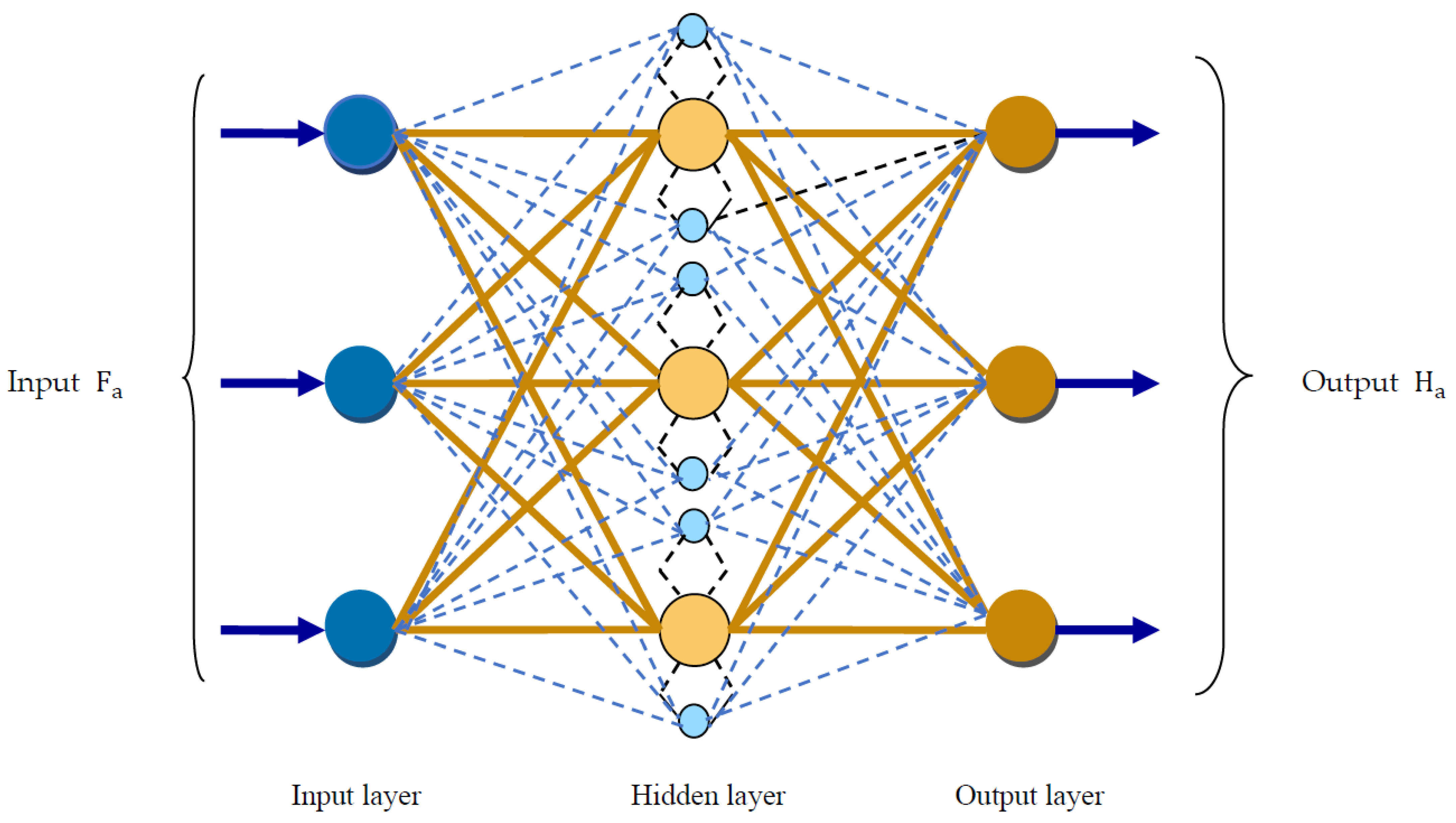
3.6. Object Recognition Using Proposed FP-SFOA

The extracted feature $F_a$ is subjected to the object-recognition stage, where objects are identified employing the DQN classifier. The training of DQN is efficiently conducted using the proposed FP-SFOA, which includes the incorporation of the FC concept with PO [26,30] and SFOA [29].

• Architecture of DQN

A combination of deep learning (DL) and reinforcement learning (RL) was successfully used to introduce a fascinating network that surpasses all other neural networks, named DQN [37]. This DQN is very popular in solving most of the highly dimensional optimization problems. Moreover, this network consists of a deep convolution neural network for $Q$-function approximation, whereas mini-batches are employed for uneven training data. The remaining network parameters are utilized to estimate the $Q$-values of the next state. The architectural diagram of DQN is portrayed in Figure 5. The feature vector $F_a$ is applied over DQN for a given state $Nn, jj$ vector of action value $Q\left(Nn, jj; \theta \right)$, in which $\theta$ shows the learning factor of DQN. In addition, the loss parameter of DQN is computed using the below expression:

$$Los{s}_{ii}\hspace{0.17em}\left({\theta }_{ii}\right)=E_{Nn,\hspace{0.17em}jj,\hspace{0.17em}\varpi ,\hspace{0.17em}N{n}^{\prime }}\hspace{0.17em}\left[{\left(L_{ii}-Q\hspace{0.17em}\left(Nn,\hspace{0.17em}jj,\hspace{0.17em}{\theta }_{ii}\right)\right)}^2\right]$$

(35)

where

$$L_{ii}=\left({\varpi }_{ii}+\lambda {\max }_{j{j}^{\prime }}\hspace{0.17em}Q\hspace{0.17em}\left(N{n}^{\prime },\hspace{0.17em}j{j}^{\prime },\hspace{0.17em}{\theta }^{-}\right)\right)$$

(36)

The obtained error is denoted as ${\mathrm{Loss}}_{\mathrm{ii}}$ if the factor is ${\theta }_{ii}$ Here, ${\theta }^{-}$ refers to the factors of a partitioned target structure, and the online structure factors are specified as ${\theta }_{ii}$. The gradient descent function is expressed in the following manner:

$${\nabla }_{{\theta }_{ii}}\hspace{0.17em}Los{s}_{ii}\hspace{0.17em}\left({\theta }_{ii}\right)={{\rm E}}_{Nn,\hspace{0.17em}jj,\hspace{0.17em}\varpi ,\hspace{0.17em}N{n}^{\prime }}\hspace{0.17em}\left[\left(L_{ii}-Q\hspace{0.17em}\left(Nn,\hspace{0.17em}jj;\hspace{0.17em}{\theta }_{ii}\right)\right)\hspace{0.17em}{\nabla }_{{\theta }_{ii}}\hspace{0.17em}Q\hspace{0.17em}\left(Nn,\hspace{0.17em}jj\right)\right]$$

(37)

In order to discard the associated updates, both the experience replay and constant maximal volume are fed to DQN. Thus, the divergence problem is solved in an effective way, and the recognized object result obtained from DQN is illustrated as $H_a.$

ii.

Training of DQN using FP-SFOA

The parameters of DQN are optimally tuned using FP-SFOA; thus, the optimal solution for the recognized object result is attained. However, the introduction of hybrid algorithms results in superior performance with a high convergence speed that can easily solve the highly dimensional optimization problem.

Fractional political position encoding

This is used to determine the finest solution for a given optimization problem in a $\mathrm{G}$-dimensional search area, such that $G=\left[1\times \theta \right]$. Here, $\theta$ refers to the learning parameter of DQN.

Fitness function

The fitness factor is employed to find the finest solution, which is described as the change in variation amongst the targeted result and outcome of DQN.

$$\Im =\frac{1}{b}\hspace{0.17em}{\displaystyle \sum _{a=1}^b\left[{\tau }_a-H_a\right]{\hspace{0.17em}}^2}$$

(38)

where $b$ symbolizes the overall quantity of image samples, ${\tau }_a$ is the targeted outcome, and the output of DQN is signified as $H_a$.

The algorithmic steps of FP-SFOA are the same as that of PSFOA, which is already elaborated under Section 3.1.2.

The updated solution of PSFOA is given by

$$X_{new,\hspace{0.17em}S}^{i+1}\hspace{0.17em}=\frac{X_S^{i-1}\hspace{0.17em}\left(R-1\right)\hspace{0.17em}\left(1-c\times \mathit{Sin}\hspace{0.17em}\left(\omega \right)\right)+R.c\times \mathit{Sin}\hspace{0.17em}\left(\omega \right)\hspace{0.17em}\left(X_{best,\hspace{0.17em}S}^i\right)}{R-1+c\times \mathit{Sin}\hspace{0.17em}\left(\omega \right)}$$

(39)

In order to apply the FC concept, $X_{S, old}^{ i}$ is subtracted on both sides, and the equation becomes

$$X_{new,\hspace{0.17em}S}^{i+1}-X_{S,\hspace{0.17em}old}^i\hspace{0.17em}=\frac{X_S^{i-1}\hspace{0.17em}\left(R-1\right)\hspace{0.17em}\left(1-c\times \mathit{Sin}\hspace{0.17em}\left(\omega \right)\right)+R.c\times \mathit{Sin}\hspace{0.17em}\left(\omega \right)\hspace{0.17em}\left(X_{best,\hspace{0.17em}S}^i\right)}{R-1+c\times \mathit{Sin}\hspace{0.17em}\left(\omega \right)}-X_{S,\hspace{0.17em}old}^i$$

(40)

By applying the FC concept,

$$D^{\hslash }\hspace{0.17em}\left[X_{new,\hspace{0.17em}S}^{i+1}\right]=\frac{X_S^{i-1}\hspace{0.17em}\left(R-1\right)\hspace{0.17em}\left(1-c\times \mathit{Sin}\hspace{0.17em}\left(\omega \right)\right)+R.c\times \mathit{Sin}\hspace{0.17em}\left(\omega \right)\hspace{0.17em}\left(X_{best,\hspace{0.17em}S}^i\right)}{R-1+c\times \mathit{Sin}\hspace{0.17em}\left(\omega \right)}-X_{S,\hspace{0.17em}old}^i$$

(41)

$$X_{new,\hspace{0.17em}S}^{i+1}-\hslash \hspace{0.17em}{X}_{old,\hspace{0.17em}S}^i-\frac{1}{2}\hspace{0.17em}\hslash \hspace{0.17em}{X}_S^{i-1}-\frac{1}{6}\hspace{0.17em}\left(1-\hslash \right)\hspace{0.17em}{X}_S^{i-2}-\frac{1}{24}\hspace{0.17em}\hslash \hspace{0.17em}\left(1-\hslash \right)\hspace{0.17em}\left(2-\hslash \right)\hspace{0.17em}{X}_S^{i-3}=\frac{X_S^{i-1}\hspace{0.17em}\left(R-1\right)\hspace{0.17em}\left(1-c\times \mathit{Sin}\hspace{0.17em}\left(\omega \right)\right)+R.c\times \mathit{Sin}\hspace{0.17em}\left(\omega \right)\hspace{0.17em}\left(X_{best,\hspace{0.17em}S}^i\right)}{R-1+c\times \mathit{Sin}\hspace{0.17em}\left(\omega \right)}-X_{S,\hspace{0.17em}old}^i$$

(42)

Hence, the updated solution of FP-SFOA is represented as

$$X_{new,\hspace{0.17em}S}^{i+1}=\left(\hslash -1\right)\hspace{0.17em}{X}_{old,\hspace{0.17em}S}^i+\frac{1}{2}\hspace{0.17em}\hslash \hspace{0.17em}{X}_S^{i-1}-\frac{1}{6}\hspace{0.17em}\left(1-\hslash \right)\hspace{0.17em}{X}_S^{i-2}-\frac{1}{24}\hspace{0.17em}\hslash \hspace{0.17em}\left(1-\hslash \right)\hspace{0.17em}\left(2-\hslash \right)\hspace{0.17em}{X}_S^{i-3}+\frac{X_S^{i-1}\hspace{0.17em}\left(R-1\right)\hspace{0.17em}\left(1-c\times \mathit{Sin}\hspace{0.17em}\left(\omega \right)\right)+R.c\times \mathit{Sin}\hspace{0.17em}\left(\omega \right)\hspace{0.17em}\left(X_{best,\hspace{0.17em}S}^i\right)}{R-1+c\times \mathit{Sin}\hspace{0.17em}\left(\omega \right)}$$

(43)

where $X_S^{i-1}, X_S^{i-2}$, and $X_S^{i-3}$ represent the $S\mathrm{th}$ component of the length of the sunflower stem at the $\left(i-1\right)\mathrm{th}, \left(i-2\right)\mathrm{th}$, and $\left(i-3\right)\mathrm{th}$ iteration, respectively. Moreover, the maximum number of iterations is specified as $i_{\max }$, while the damping parameter is notated as $C$.

3.7. Aggregation at the Server Using CAViaR Model

Each local node generates a weight, and these local nodes are collectively known as the local model. The weights from the local model are aggregated at the global model, which is a server, and the aggregation process at the global model is effectively conducted using the CAViaR model.

The CAViaR model [25] defines the evolution of the quantile over a time period utilizing an autoregressive mechanism and determines the factors with regression quantiles. Let us consider the weight of the global model as $W_{\mathit{global}}$, and it is expressed as

$$W_{global}=\left\{W_{loc1},\hspace{0.17em}{W}_{loc2},\dots ,W_{loc\hspace{0.17em}n}\right\}$$

(44)

Here, $W_{loc, n}$ represents the $n\mathrm{th}$ weight of the local node, which is the total quantity of local nodes present in the local model.

Applying the CAViaR model to the local node $W_{loc, n}$, the expression is computed as follows:

$$W_{global}={\beta }_0+{\beta }_1\hspace{0.17em}{W}_{loc1}\hspace{0.17em}\left(q-1\right)+{\beta }_2\hspace{0.17em}{W}_{loc2}\left(q-2\right)+\beta \hspace{0.17em}fit\hspace{0.17em}\left(W_{loc1}\hspace{0.17em}\left(q-1\right)\right)+{\beta }_2\hspace{0.17em}fit\hspace{0.17em}\left(W_{loc2}\hspace{0.17em}\left(q-2\right)\right)$$

(45)

Here, the weight of local mode 1 at the $\left(q-1\right)\mathrm{th}$ iteration and the weight of local node 2 at the $\left(t-2\right)\mathrm{th}$ iteration is denoted as $W_{\mathit{loc}1}\left(q-1\right)$ and $W_{\mathit{loc}2}\left(q-1\right)$, respectively. The pvector of unknown parameter is indicated as $\beta$. Moreover, the fitness of value of weight at the $\left(q-1\right)$ iteration is termed $fit(W_{\mathit{loc}1}\left(q-1)\right)$, and $fit(W_{\mathit{loc}2}\left(q-2)\right)$ is the fitness of value of weight at the $\left(q-2\right)$ iteration.

3.8. Apply Global Training Model to Every Local Node

After averaging the weights at the global model using the CAViaR model, the averaged weights are updated at every local node at the local model. This global training model can decrease the computational time and enhance the efficiency of the designed system.

4. Results and Discussion

A discussion of the results of FP-SFOA-DQN-FL and a comparison with existing models can help to prove the efficacy of the designed model, which is interpreted in this section.

4.1. Experimental Setup

The demonstration of this research work is carried out using the MATLAB tool.

Table 2. Parameter details.

Parameters	Values
Learning rate	0.01
Batch size	32
Epoch	50

shows the parameters of FP-SFOA-DQN-FL.

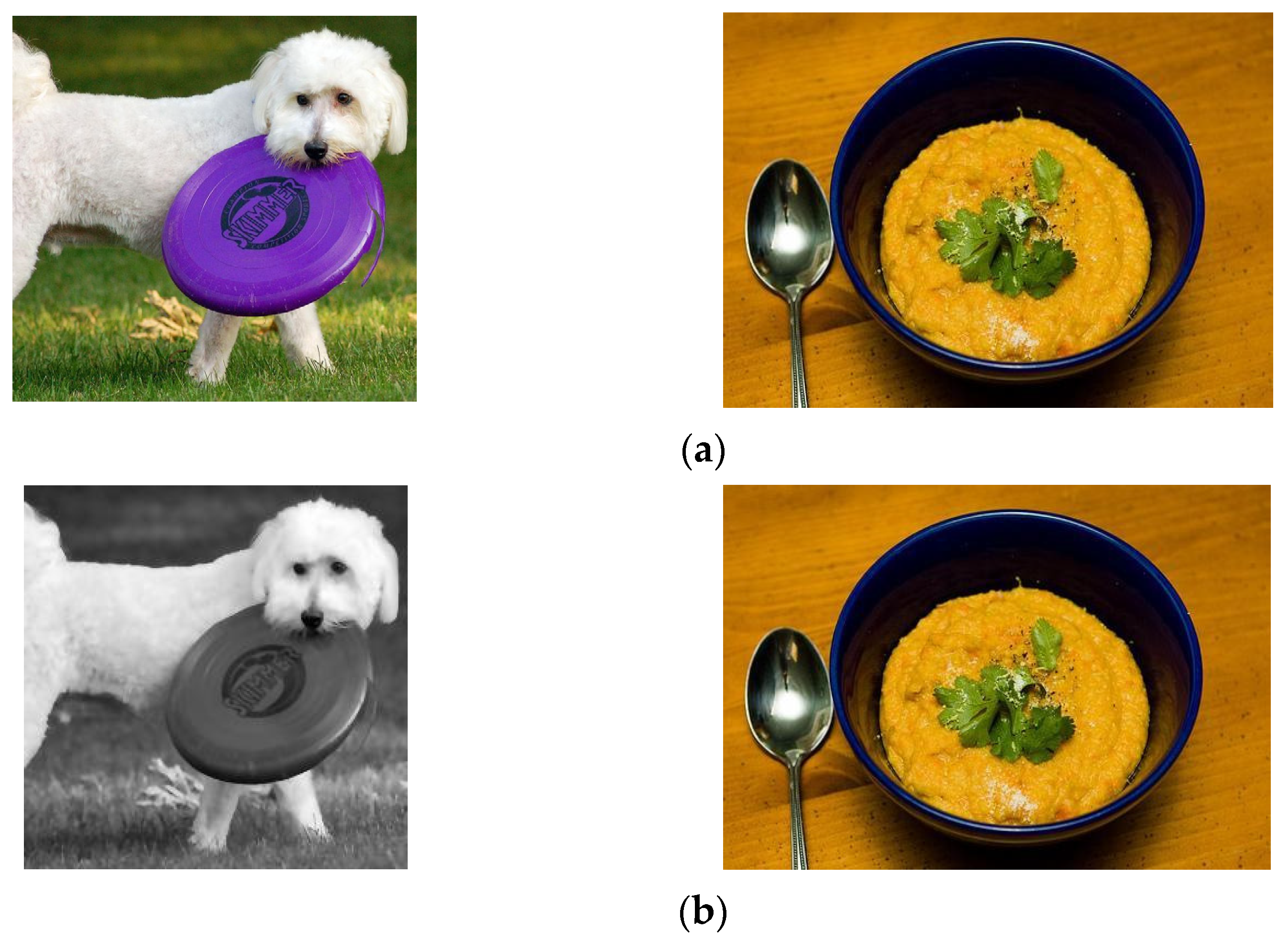
4.2. Dataset Description

The datasets used for the implementation of FP-SFOA-DQN-FL are the YOLO object-detection dataset and the MyNursingHome dataset.

4.2.1. YOLO Object-Detection Dataset

This dataset [38] consists of five classes, which includes animals, food, human, bird, and object. In addition, the overall file size of this YOLO-coco dataset is 6 GB.

4.2.2. MyNursingHome Dataset

This dataset [24] is a fully labeled image dataset collected from elder home cares situated in Malaysia utilized for the purpose of image detection and classification. This repository includes 37,500 images from 25 diverse indoor objects generally available in homes, such as beds, benches, walkers, chairs, tables, and wheelchairs.

4.3. Experimental Results

The experimental results of this research are shown in Figure 6. The input images are given in Figure 6a, and the corresponding filtered and object-detection outputs are depicted in Figure 6b and Figure 6c, respectively.

4.4. Evaluation Metrices

The evaluation metrics considered for experimentation of FP-SFOA-DQN-FL are defined as follows:

4.4.1. Accuracy

Accuracy is the capability of a measure to match the original value of the quantity being estimated.

4.4.2. Loss Function

A loss function is defined as a function that represents an event of more than one variable, illustrating certain costs corresponding to the event. In order to mitigate the loss function, optimization is used.

4.4.3. Mean Square Error (MSE)

The MSE is described as the mean squared error between actual values and expected outcomes, and it is computed using Equation (38).

4.4.4. Root Mean Square Error (RMSE)

The RMSE is defined as the average deviation of the estimations from the observed values, and it is the square root of the mean square error.

$$RMSE=\sqrt{\frac{1}{b}\hspace{0.17em}{\displaystyle \sum _{a=1}^b\left[{\tau }_a-H_a\right]{\hspace{0.17em}}^2}}$$

(46)

4.4.5. False-Positive Rate (FPR)

The FPR is the proportion of the number of negative objects wrongly detected of the total count of actual negative objects, and it is given by

$$FPR=\frac{F_p}{F_p+T_n}$$

(47)

Here, $F_p$ and $T_n$ denote as false-positive and true-negative, respectively.

4.4.6. Mean Average Precision

This is employed to calculate the performance of systems performing an object-detection process.

4.4.7. Communication Cost

The communication cost is determined by the division of bytes from the local server to the global server with a normalization factor.

4.5. Performance Analysis

The performance of FP-SFOA-DQN-FL is analyzed by varying the epochs, and the results are depicted in this section.

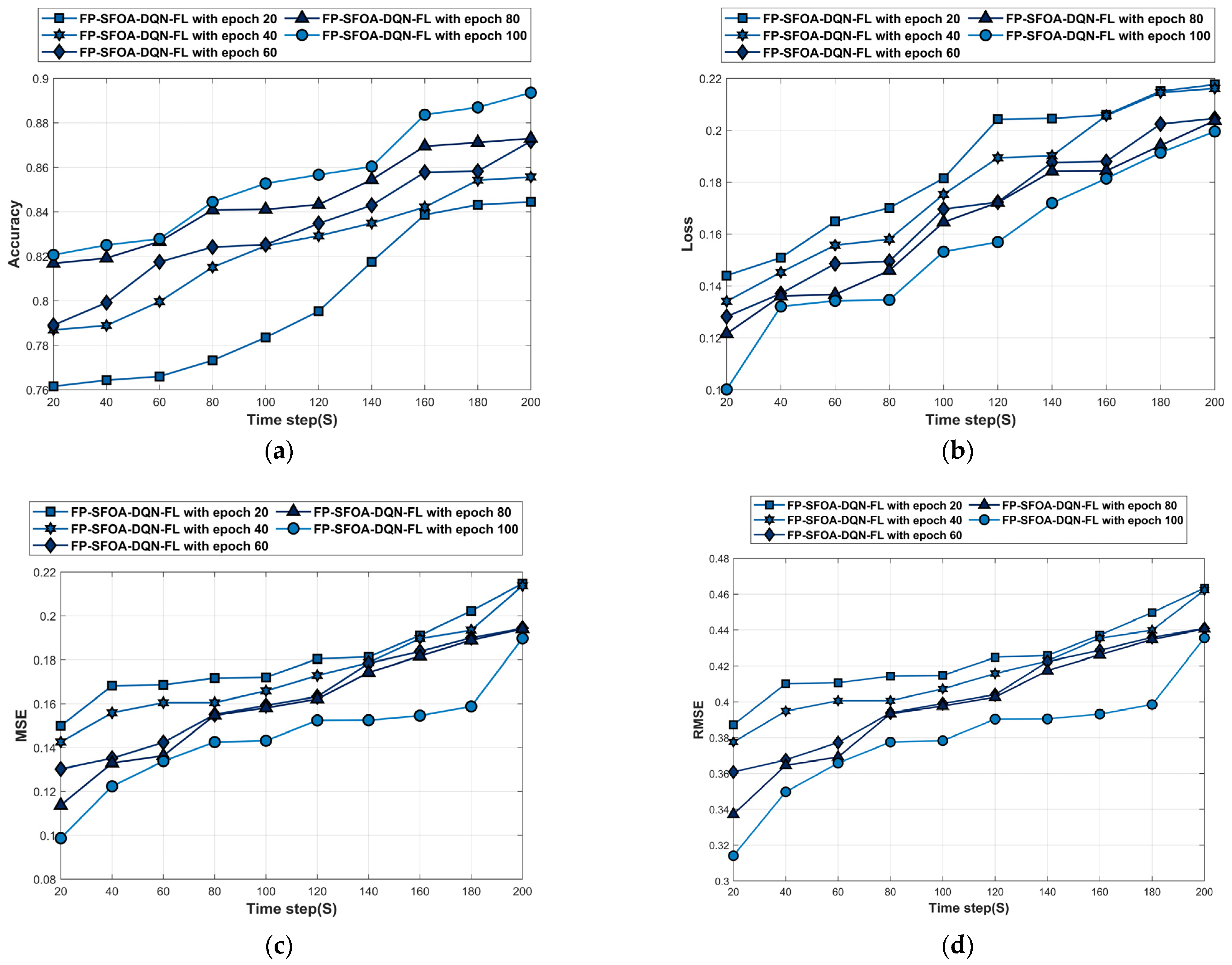
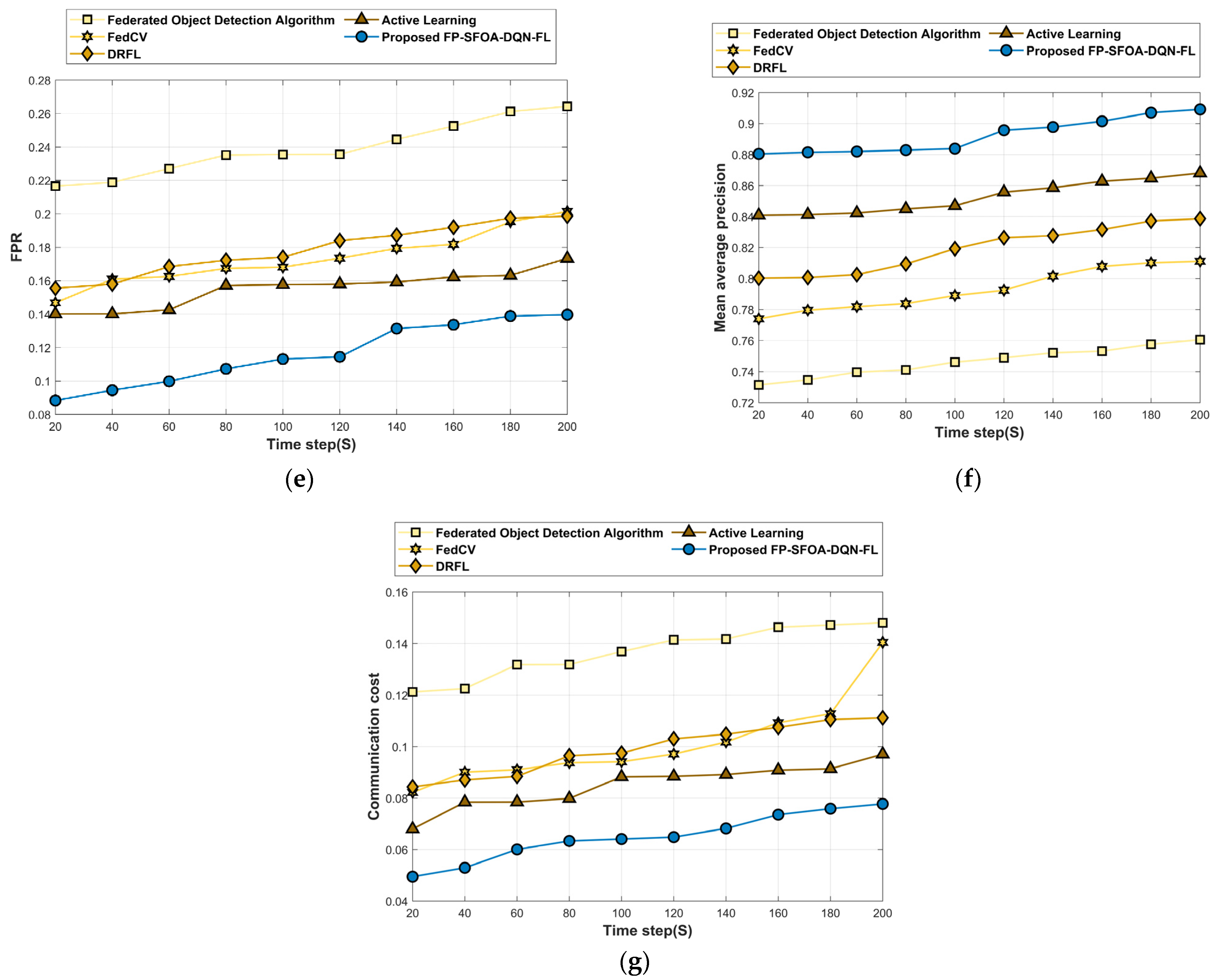
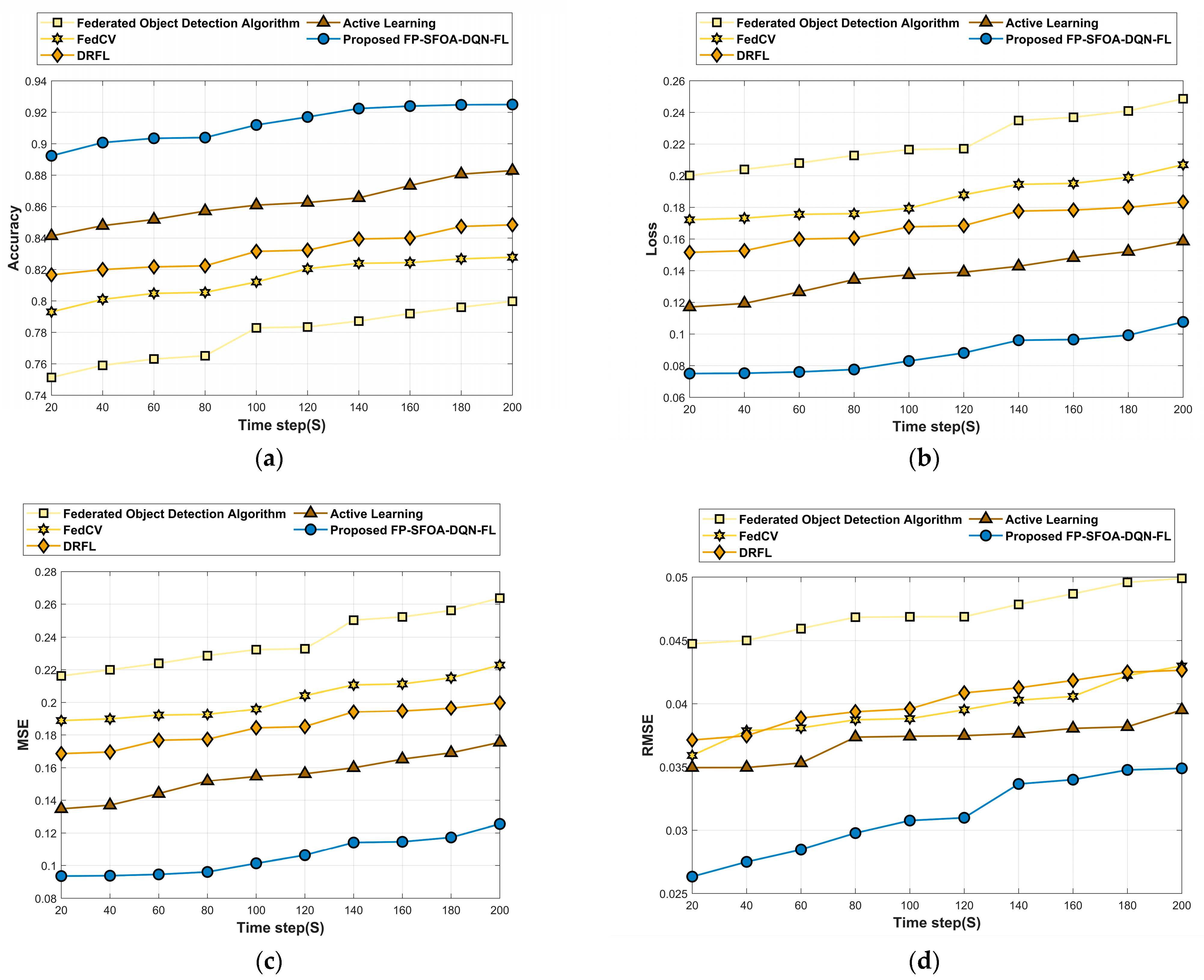
4.5.1. Performance Analysis Based on YOLO Object-Detection Dataset

The analysis of the YOLO object-detection dataset is depicted in Figure 7. Figure 7a denotes the accuracy analysis of FP-SFOA-DQN-FL. For time step = 100 s, the accuracy of the FP-SFOA-DQN-FL at epochs 20, 40, 60, 80, and 100 is 0.783, 0.825, 0.825, 0.841, and 0.853. The loss analysis of FP-SFOA-DQN-FL is given in Figure 7b. The loss of FP-SFOA-DQN-FL at epochs 20, 40, 60, 80, and 100 is 0.206, 0.206, 0.188, 0.184, and 0.181 for time stamp = 160 s. Figure 7c denotes the MSE analysis of FP-SFOA-DQN-FL. For time step = 120 s, the MSE of FP-SFOA-DQN-FL at epochs 20, 40, 60, 80, and 100 is 0.180, 0.173, 0.163, 0.162, and 0.152. The RMSE analysis of FP-SFOA-DQN-FL is given in Figure 7d. The RMSE of FP-SFOA-DQN-FL at epochs 20, 40, 60, 80, and 100 is 0.463, 0.462, 0.441, 0.441, and 0.436 for time stamp = 200 s. Figure 7e denotes the FPR analysis of FP-SFOA-DQN-FL. For time step = 100 s, the FPR of FP-SFOA-DQN-FL at epochs 20, 40, 60, 80, and 100 is 0.206, 0.193, 0.191, 0.180, and 0.179. The mean average precision analysis of FP-SFOA-DQN-FL is given in Figure 7f. The mean average precision of FP-SFOA-DQN-FL at epochs 20, 40, 60, 80, and 100 is 0.812, 0.819, 0.835, 0.866, and 0.870 for time stamp = 140 s.

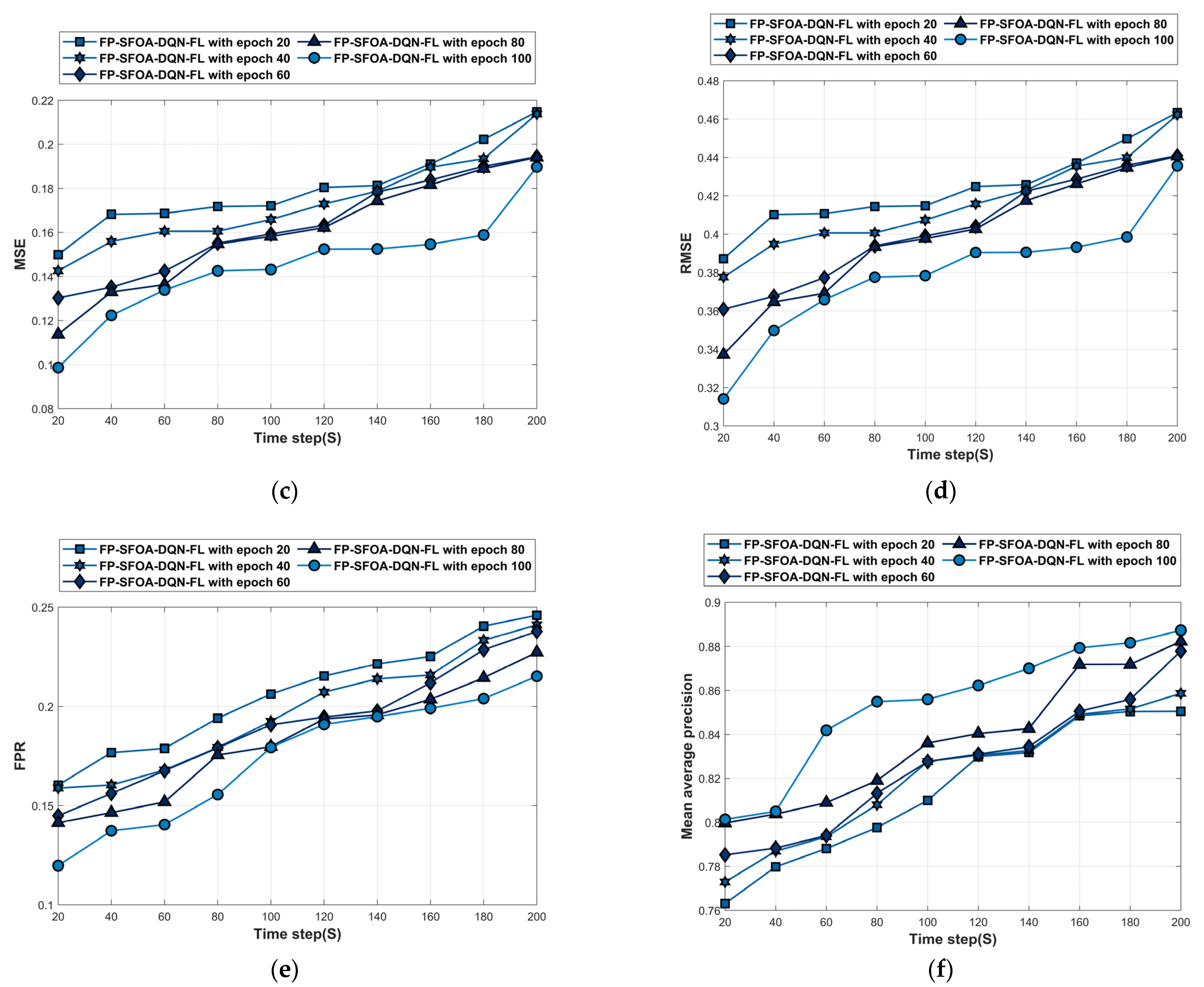
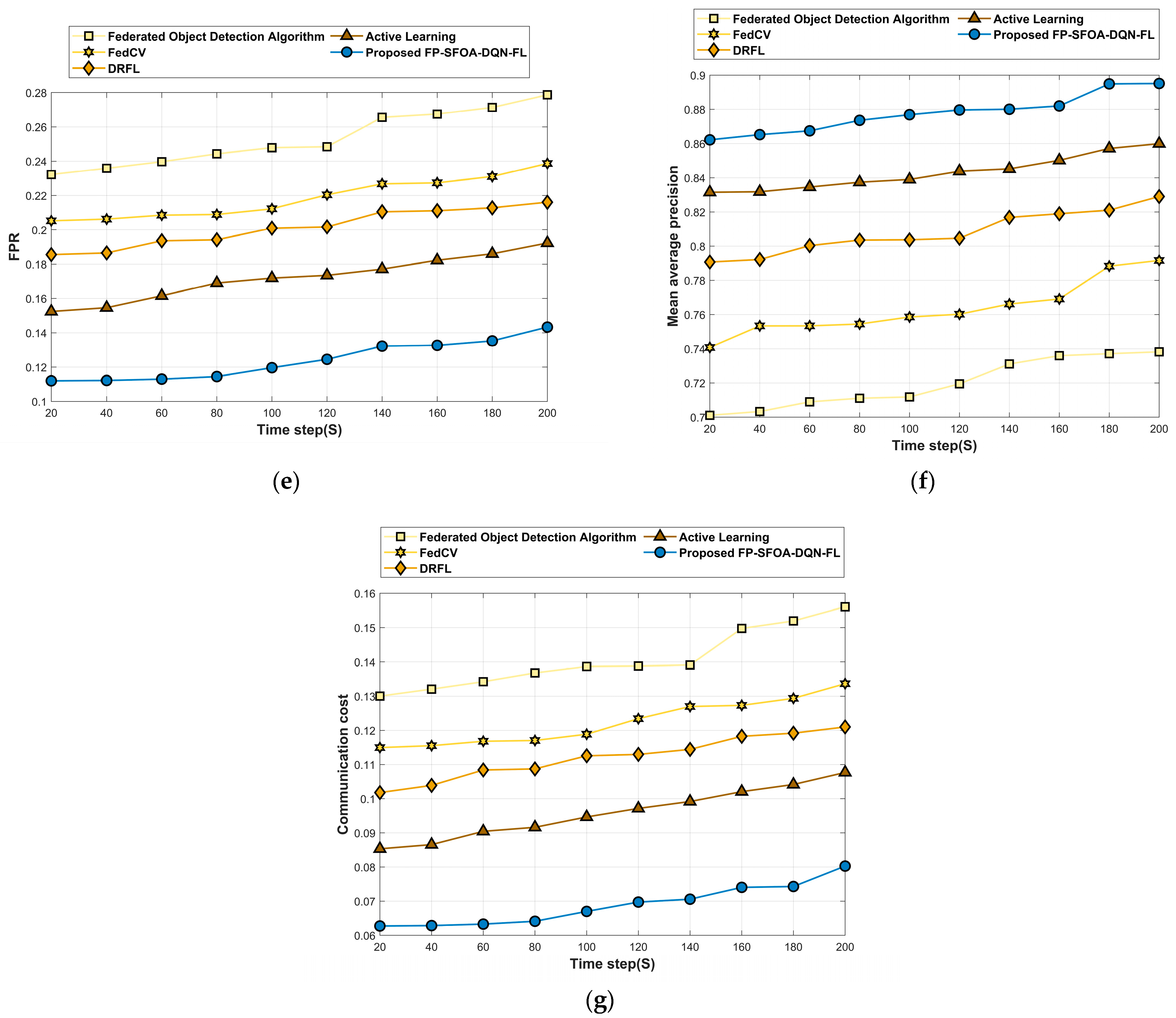
4.5.2. Performance Analysis Based on MyNursingHome Dataset

Figure 8 depicts the analysis of the MyNursingHome dataset. Figure 8a denotes the accuracy analysis of FP-SFOA-DQN-FL. For time step = 200 s, the accuracy of FP-SFOA-DQN-FL at epochs 20, 40, 60, 80, and 100 is 0.844, 0.856, 0.872, 0.873, and 0.894. The loss analysis of FP-SFOA-DQN-FL is given in Figure 8b. The loss of the FP-SFOA-DQN-FL at epochs 20, 40, 60, 80, and 100 is 0.205, 0.190, 0.188, 0.184, and 0.172 for time stamp = 140 s. Figure 8c denotes the MSE analysis of FP-SFOA-DQN-FL. For time step = 80 s, the MSE of FP-SFOA-DQN-FL at epochs 20, 40, 60, 80, and 100 is 0.172, 0.161, 0.155, 0.155, and 0.143. The RMSE analysis of FP-SFOA-DQN-FL is given in Figure 8d. The RMSE of FP-SFOA-DQN-FL at epochs 20, 40, 60, 80, and 100 is 0.463, 0.462, 0.441, 0.441, and 0.436 for time stamp = 200 s. Figure 8e denotes the FPR analysis of FP-SFOA-DQN-FL. For time step = 100 s, the FPR of FP-SFOA-DQN-FL at epochs 20, 40, 60, 80, and 100 is 0.206, 0.193, 0.191, 0.180, and 0.179. The mean average precision analysis of FP-SFOA-DQN-FL is given in Figure 8f. The mean average precision of FP-SFOA-DQN-FL at epochs 20, 40, 60, 80, and 100 is 0.850, 0.859, 0.878, 0.882, and 0.887 for time stamp = 200 s.

4.6. Comparative Methods

The performance of FP-SFOA-DQN-FL was analyzed and compared with former techniques, like the federated object-detection algorithm [1], FedCV [9], DRFL [19], and active learning [20].

4.7. Comparative Evaluation

This part delineates the estimation of FP-SFOA-DQN-FL in accordance with the evaluation measures based on two datasets by varying the time step from 20 to 200.

4.7.1. Analysis Based on YOLO Object-Detection Dataset

This analysis section describes the assessment of FP-SFOA-DQN-FL based on the YOLO object-detection dataset depicted in Figure 9. Figure 9a specifies the evaluation of FP-SFOA-DQN-FL with respect to accuracy. If the time step is 200 s, the accuracy gained by FP-SFOA-DQN-FL is 0.950, while the existing models gained an accuracy of 0.816 for the federated object-detection algorithm, 0.889 for FedCV, 0.880 for DRFL, and 0.896 for active learning. While considering the time step as 200 s, the loss function attained by the designed approach illustrated in Figure 9b is 0.104, and MSE gained by FP-SFOA-DQN-FL is 0.122, as shown in Figure 9c. However, the existing models delivered the MSE as 0.249, 0.185, 0.182, and 0.156, respectively, for the federated object-detection algorithm, FedCV, DRFL, and active learning. Figure 9d implies the evaluation of RMSE. By considering the time step as 200 s, the RMSE received by the proposed FP-SFOA-DQN-FL is 0.035, and the FPR attained by the designed scheme is 0.140, as illustrated in Figure 9e. Also, the FPR provided by conventional schemes, like the federated object-detection algorithm, is 0.264, FedCV is 0.201, DRFL is 0.199, and active learning is 0.173. Figure 9f signifies the comparative evaluation of FP-SFOA-DQN-FL in terms of mean average precision. When the time step was 200 s, FP-SFOA-DQN-FL delivered a mean average precision of 0.909. Figure 9g depicts the comparative evaluation of communication cost. When the time step was 100 s, the communication cost of the federated object-detection algorithm, FedCV, DRFL, active learning, and FP-SFOA-DQN-FL was 0.137, 0.094, 0.097, 0.088, and 0.064, respectively.

4.7.2. Evaluation Based on MyNursingHome Dataset

Figure 10 delineates the assessment of FP-SFOA-DQN-FL based on the MyNursingHome dataset with respect to evaluation indicators. Figure 10a signifies the evaluation of FP-SFOA-DQN-FL in accordance with accuracy. By increasing the time step from 20 s to 200 s, the accuracy profited by the developed technique was 0.925, while the classical approaches attained a loss function of 0.249 for the federated object-detection algorithm, 0.207 for FedCV, 0.183 for DRFL and 0.159 for active learning as shown in Figure 10b. Figure 10c depicts the evaluation of the devised methodology in accordance with MSE. When assuming the time step as 200 s, the MSE obtained by FP-SFOA-DQN-FL was 0.125. Figure 10d implies the evaluation of RMSE. By considering the time step as 200 s, the RMSE received by the proposed FP-SFOA-DQN-FL was 0.034, and the FPR attained by the designed scheme was 0.143, as specified in Figure 10e. Also, the FPR provided by the existing models, such as the federated object-detection algorithm, is 0.279, FedCV is 0.239, DRFL is 0.216, and active learning is 0.192. Figure 10f implies the comparative evaluation of FP-SFOA-DQN-FL in terms of mean average precision. When the time step was 200 s, FP-SFOA-DQN-FL delivered a mean average precision of 0.895. The comparative evaluation of communication cost is depicted in Figure 10g. When the time step was 100 s, the communication cost of the federated object-detection algorithm, FedCV, DRFL, active learning, and FP-SFOA-DQN-FL was 0.150, 0.127, 0.118, 0.102, and 0.074, respectively.

4.8. Comparative Discussion

The discussion of FP-SFOA-DQN-FL is depicted in

Table 3. Comparative discussion.

Datasets	Time Step	Metrics/ Methods	Federated Object Detection	FedCV	DRFL	Active Learning	FP-SFOA-DQN-FL
		Accuracy	0.816	0.889	0.880	0.896	0.950
		Loss function	0.234	0.168	0.165	0.139	0.104
Dataset-1		MSE	0.249	0.185	0.182	0.156	0.122
	Time Step = 200 s	RMSE	0.050	0.043	0.043	0.040	0.035
		FPR	0.264	0.201	0.199	0.173	0.140
		Mean average Precision	0.761	0.811	0.839	0.868	0.909
		Communication cost	0.148	0.140	0.111	0.097	0.078
		Accuracy	0.800	0.828	0.848	0.883	0.925
		Loss function	0.249	0.207	0.183	0.159	0.108
Dataset-2		MSE	0.264	0.223	0.200	0.175	0.125
	Time Step = 200 s	RMSE	0.049	0.042	0.042	0.039	0.034
		FPR	0.279	0.239	0.216	0.192	0.143
		Mean average Precision	0.738	0.792	0.829	0.860	0.895
		Communication cost	0.156	0.134	0.121	0.108	0.080

. It is crystal clear that FP-SFOA-DQN-FL has attained high accuracy of 0.950, low loss function of 0.104, low MSE of 0.122, minimum RMSE of 0.035, minimum FPR of 0.140, and maximum average precision of 0.909 based on dataset-1 at time step = 200 s.

4.9. Analysis of Computational Time

The computational time of the models is discussed in

Table 4. Computational time.

Methods	Federated Object Detection	FedCV	DRFL	Active Learning	FP-SFOA-DQN-FL
Computational time (sec)	9.521478523	8.255785244	7.258746581	6.258744698	5.254789502

. The computational time of the implemented FP-SFOA-DQN-FL is compared with the federated object detection, FedCV, DRFL, and active learning methods, in which minimal computational time is required for the devised method.

5. Conclusions

FL is basically machine learning, where the prime objective is to tune a high-standard centralized system while data are distributed over a huge number of devices with slow network connections. This research introduces an effective FL model for real-world object recognition using designed FP-SFOA. In each round, local training is performed based on local data at every node, and the object-recognition process is performed at the training model of every node. In the training model, the input indoor image is pre-processed utilizing a bilateral filter to eliminate the calamities, and following this, object recognition is conducted employing SegNet, which is tuned by exploiting PSFOA. After, features like ResNet features, SLBT, GLCM, SIFT, SURF, ORB, and hierarchical skeleton features are extracted, and finally, object identification is performed based on FP-SFOA. Finally, the weights from every local node are aggregated at the global model using CAViaR, and then the aggregated weights are updated back to the global model. The devised FP-SFOA delivered a maximum accuracy and mean average precision of 0.950 and 0.909, whereas it gained a minimum loss function of 0.104, MSE of 0.122, RMSE of 0.035, FPR of 0.140, and communication cost of 0.078. The designed FL framework delivered superior performance and outperformed other classical models. Despite its magnificent results, some of the features during the feature extraction module consumed time to compute the feature vector, which resulted in inaccurate results on blurring images. This drawback will be considered in further research.

References

1. Luo, J.; Wu, X.; Luo, Y.; Huang, A.; Huang, Y.; Liu, Y.; Yang, Q. Real-world image datasets for federated learning. arXiv 2019, arXiv:1910.11089. [Google Scholar]
2. Hussain, F.; Hassan, S.A.; Hussain, R.; Hossain, E. Machine learning for resource management in cellular and IoT networks: Potentials, current solutions, and open challenges. IEEE Commun. Surv. Tutor. 2020, 22, 1251–1275. [Google Scholar] [CrossRef]
3. Konečný, J.; McMahan, H.B.; Yu, F.X.; Richtárik, P.; Suresh, A.T.; Bacon, D. Federated learning: Strategies for improving communication efficiency. arXiv 2016, arXiv:1610.05492. [Google Scholar]
4. Deng, J.; Guo, J.; Ververas, E.; Kotsia, I.; Zafeiriou, S. Retinaface: Single-shot multi-level face localisation in the wild. In Proceedings of the IEEE/CVF Conference on Computer Vision and Pattern Recognition, Seattle, WA, USA, 13–19 June 2020. [Google Scholar]
5. Mittal, M.; Verma, A.; Kaur, I.; Kaur, B.; Sharma, M.; Goyal, L.M.; Roy, S.; Kim, T.-H. An Efficient Edge Detection Approach to Provide Better Edge Connectivity for Image Analysis. IEEE Access 2019, 7, 33240–33255. [Google Scholar] [CrossRef]
6. Lin, T.Y.; Goyal, P.; Girshick, R.; He, K.; Dollár, P. Focal loss for dense object detection. In Proceedings of the IEEE International Conference on Computer Vision, Venice, Italy, 22–29 October 2017. [Google Scholar]
7. Ren, S.; He, K.; Girshick, R.; Sun, J. Faster r-cnn: Towards real-time object detection with region proposal networks. Adv. Neural Inf. Process. Syst. 2015, 28. [Google Scholar] [CrossRef]
8. Liu, Y.; Huang, A.; Luo, Y.; Huang, H.; Liu, Y.; Chen, Y.; Feng, L.; Chen, T.; Yu, H.; Yang, Q. Federated learning-powered visual object detection for safety monitoring. AI Mag. 2021, 42, 19–27. [Google Scholar] [CrossRef]
9. He, C.; Shah, A.D.; Tang, Z.; Sivashunmugam, D.F.N.; Bhogaraju, K.; Shimpi, M.; Shen, L.; Chu, X.; Soltanolkotabi, M. Fedcv: A federated learning framework for diverse computer vision tasks. arXiv 2021, arXiv:2111.11066. [Google Scholar]
10. Bayar, B.; Stamm, M.C. A deep learning approach to universal image manipulation detection using a new convolutional layer. In Proceedings of the 4th ACM Workshop on Information Hiding and Multimedia Security, Vigo, Spain, 20–22 June 2016. [Google Scholar]
11. Karpathy, A.; Li, F.-F. Deep visual-semantic alignments for generating image descriptions. In Proceedings of the IEEE Conference on Computer Vision and Pattern Recognition, Boston, MA, USA, 7–12 June 2015. [Google Scholar]
12. He, K.; Zhang, X.; Ren, S.; Sun, J. Deep residual learning for image recognition. In Proceedings of the IEEE Conference on Computer Vision and Pattern Recognition, Las Vegas, NV, USA, 26 June–1 July 2016. [Google Scholar]
13. Mabrouk, A.; Redondo, R.P.D.; Elaziz, M.A.; Kayed, M. Ensemble Federated Learning: An approach for collaborative pneumonia diagnosis. Appl. Soft Comput. 2023, 144, 110500. [Google Scholar] [CrossRef]
14. Alam, M.; Ahmed, T.; Hossain, M.; Emo, M.H.; Bidhan, K.I.; Reza, T.; Alam, G.R.; Hassan, M.M.; Pupo, F.; Fortino, G. Federated ensemble-learning for transport mode detection in vehicular edge network. Futur. Gener. Comput. Syst. 2023, 149, 89–104. [Google Scholar] [CrossRef]
15. Yeganeh, A.; Pourpanah, F.; Shadman, A. An ANN-based ensemble model for change point estimation in control charts. Appl. Soft Comput. 2021, 110, 107604. [Google Scholar] [CrossRef]
16. Mohammed, A.; Kora, R. A comprehensive review on ensemble deep learning: Opportunities and challenges. J. King Saud Univ.-Comput. Inf. Sci. 2023, 35, 757–774. [Google Scholar] [CrossRef]
17. Ye, Y.; Li, S.; Liu, F.; Tang, Y.; Hu, W. EdgeFed: Optimized federated learning based on edge computing. IEEE Access 2020, 8, 209191–209198. [Google Scholar] [CrossRef]
18. Chen, X.; Zhang, H.; Wu, C.; Mao, S.; Ji, Y.; Bennis, M. Optimized computation offloading performance in virtual edge computing systems via deep reinforcement learning. IEEE Internet Things J. 2018, 6, 4005–4018. [Google Scholar] [CrossRef]
19. Zhu, R.; Yin, K.; Xiong, H.; Tang, H.; Yin, G. Masked face detection algorithm in the dense crowd based on federated learning. Wirel. Commun. Mob. Comput. 2021, 2021, 8586016. [Google Scholar] [CrossRef]
20. van Bommel, J. Active Learning during Federated Learning for Object Detection; University of Twente Enschede: Enschede, The Netherlands, 2021. [Google Scholar]
21. Yu, P.; Liu, Y. Federated object detection: Optimizing object detection model with federated learning. In Proceedings of the 3rd International Conference on Vision, Image and Signal Processing, Vancouver, BC, Canada, 26–28 August 2019. [Google Scholar]
22. Hu, Z.; Xie, H.; Yu, L.; Gao, X.; Shang, Z.; Zhang, Y. Dynamic-aware federated learning for face forgery video detection. ACM Trans. Intell. Syst. Technol. 2022, 13, 1–25. [Google Scholar] [CrossRef]
23. Tam, P.; Math, S.; Nam, C.; Kim, S. Adaptive resource optimized edge federated learning in real-time image sensing classifications. IEEE J. Sel. Top. Appl. Earth Obs. Remote. Sens. 2021, 14, 10929–10940. [Google Scholar] [CrossRef]
24. Ismail, A.; Ahmad, S.A.; Soh, A.C.; Hassan, M.K.; Harith, H.H. MYNursingHome: A fully-labelled image dataset for indoor object classification. Data Brief 2020, 32, 106268. [Google Scholar] [CrossRef]
25. Engle, R.F.; Manganelli, S. CAViaR: Conditional autoregressive value at risk by regression quantiles. J. Bus. Econ. Stat. 2004, 22, 367–381. [Google Scholar] [CrossRef]
26. Li, T.; Sahu, A.K.; Talwalkar, A.; Smith, V. Federated learning: Challenges, methods, and future directions. IEEE Signal Process. Mag. 2020, 37, 50–60. [Google Scholar] [CrossRef]
27. Ahn, S.; Park, J.; Luo, L.; Chong, J. Adaptive Object-Region-Based Image Pre-Processing for a Noise Removal Algorithm. KSII Trans. Internet Inf. Syst. 2013, 7, 3160–3179. [Google Scholar]
28. Badrinarayanan, V.; Kendall, A.; Cipolla, R. Segnet: A deep convolutional encoder-decoder architecture for image segmentation. IEEE Trans. Pattern Anal. Mach. Intell. 2017, 39, 2481–2495. [Google Scholar] [CrossRef]
29. Sattar, D.; Salim, R. A smart metaheuristic algorithm for solving engineering problems. Eng. Comput. 2021, 37, 2389–2417. [Google Scholar] [CrossRef]
30. Askari, Q.; Younas, I.; Saeed, M. Political Optimizer: A novel socio-inspired meta-heuristic for global optimization. Knowl.-Based Syst. 2020, 195, 105709. [Google Scholar] [CrossRef]
31. Lakshmiprabha, N.; Majumder, S. Face recognition system invariant to plastic surgery. In Proceedings of the 2012 12th International Conference on Intelligent Systems Design and Applications (ISDA), IEEE, Kochi, India, 27–29 November 2012. [Google Scholar]
32. Dhivya, S.; Sangeetha, J.; Sudhakar, B. Copy-move forgery detection using SURF feature extraction and SVM supervised. Soft Comput. 2020, 24, 14429–14440. [Google Scholar] [CrossRef]
33. Bicego, M.; Lagorio, A.; Grosso, E.; Tistarelli, M. On the use of SIFT features for face authentication. In Proceedings of the 2006 Conference on Computer Vision and Pattern Recognition Workshop (CVPRW’06), IEEE, New York, NY, USA, 17–22 June 2006. [Google Scholar]
34. Bansal, M.; Kumar, M. 2D object recognition: A comparative analysis of SIFT, SURF and ORB feature descriptors. Multimed. Tools Appl. 2021, 80, 18839–18857. [Google Scholar] [CrossRef]
35. Zulpe, N.; Pawar, V. GLCM textural features for brain tumor classification. Int. J. Comput. Sci. Issues (IJCSI) 2012, 9, 354. [Google Scholar]
36. Sheeba, P.T.; Murugan, S. Fuzzy dragon deep belief neural network for activity recognition using hierarchical skeleton features. Evol. Intell. 2019, 15, 907–924. [Google Scholar] [CrossRef]
37. Sasaki, H.; Horiuchi, T.; Kato, S. A study on vision-based mobile robot learning by deep Q-network. In Proceedings of the 2017 56th Annual Conference of the Society of Instrument and Control Engineers of Japan (SICE), IEEE, Kanazawa, Japan, 19–22 September 2017. [Google Scholar]
38. YOLO Object Detection Dataset. Available online: https://www.kaggle.com/code/rahulkumarpatro/yolo-object-detection (accessed on 14 November 2022).
Figure 1. The proposed model for real-world object recognition in FL.
Applsci 13 13286 g001
Figure 2. Pictorial illustration of object-recognition process performed in the training model.
Applsci 13 13286 g002
Figure 3. Structural diagram of SegNet.
Applsci 13 13286 g003
Figure 4. Flowchart of the PSFOA.
Applsci 13 13286 g004
Figure 5. Structure of DQN.
Applsci 13 13286 g005
Figure 6. Experimental results. (a) Input images, (b) Filtered images, (c) Object-detection images.
Applsci 13 13286 g006aApplsci 13 13286 g006b
Figure 7. Performance evaluation based on YOLO object-detection dataset. (a) Accuracy, (b) Loss, (c) MSE, (d) RMSE, (e) FPR, (f) Mean average precision.
Applsci 13 13286 g007aApplsci 13 13286 g007b
Figure 8. Performance analysis based on MyNursingHome dataset. (a) Accuracy, (b) Loss, (c) MSE, (d) RMSE, (e) FPR, (f) Mean average precision.
Applsci 13 13286 g008aApplsci 13 13286 g008b
Figure 9. Comparative estimation based on YOLO object-detection dataset. (a) Accuracy, (b) Loss, (c) MSE, (d) RMSE, (e) FPR, (f) Mean average precision, (g) Communication cost.
Applsci 13 13286 g009aApplsci 13 13286 g009b
Figure 10. Comparative analysis based on MyNursingHome dataset. (a) Accuracy, (b) Loss, (c) MSE, (d) RMSE, (e) FPR, (f) Mean average precision, (g) Communication cost.
Applsci 13 13286 g010aApplsci 13 13286 g010b