Article

Congestive Heart Failure Category Classification Using Neural Networks in Short-Term Series

by
Juan L. López
1,2,*,† and
José A. Vásquez-Coronel
2,*,†
1
Centro de Innovación en Ingeniería Aplicada, Universidad Católica del Maule, Av. San Miguel 3605, Talca 3460000, Chile
2
Department of Computer Science and Industries, Universidad Católica del Maule, Av. San Miguel 3605, Talca 3460000, Chile
*
Authors to whom correspondence should be addressed.
These authors contributed equally to this work.
Appl. Sci. 2023, 13(24), 13211; https://doi.org/10.3390/app132413211
Submission received: 8 November 2023 / Revised: 29 November 2023 / Accepted: 6 December 2023 / Published: 13 December 2023
(This article belongs to the Special Issue AI, Machine Learning and Deep Learning in Signal Processing)

Abstract

:
Congestive heart failure carries immense importance in the realm of public health. This significance arises from its substantial influence on the number of lives lost, economic burdens, the potential for prevention, and the opportunity to enhance the well-being of both individuals and the broader community through decision-making in healthcare. Several researchers have proposed neural networks for classification of different congestive heart failure categories. However, there is little information about the confidence of the prediction on short-term series. Therefore, evaluating classification models is required for effective decision-making in healthcare. This paper explores the use of three classical variants of neural networks to classify three groups of patients with congestive heart failure. The study considered the iterative method Multilayer Perceptron neural network (MLP), two non-iterative models (Extreme Learning Machine (ELM) and Random Vector Functional Link Network (RVFL)), and the CNN approach. The results showed that the deep feature learning system obtained better classification rates than MLP, ELM, and RVFL. Several scenarios designed by coupling some deep feature maps with the RVFL and MLP models showed very high simulation accuracy. The overall accuracy rate of CNN–MLP and CNN–RVFL varies between 98% and 99%.

1. Introduction

Without a doubt, due to the COVID-19 pandemic, people have been subjected to high levels of stress. Likewise, the isolation generated by the health measures to control the spread of the virus has led to a sedentary lifestyle, tobacco, and a poor diet based on excess fat, salt, and sugars, among others. All these factors, which lead to diseases such as hypertension and dyslipidemia (high cholesterol), forecast an increase in the number of cases of cardiovascular disorders and, consequently, an increase in the number of deaths.
The Heart Rate Variability (HRV) analysis is a non-invasive technique that, in some cases, allows the diagnosis and prognosis of heart disease and neuropathy. Since the beginning of electrocardiography, it has been known that the heart rate changes from beat to beat (also called RR intervals). However, it was not until about 30 years ago that medical interest in this study was aroused. As HRV is related to various physiological systems, it began to be analyzed as a non-invasive technique for the diagnosis of heart disease and/or neuropathy. A common phenomenon in all clinical interpretations is that a small variability in the heart rate is a symptom of some cardiac or neurological deficiency [1]. Along with the development of applications, various analysis techniques have risen. The RR signal statistical analysis was historically the first, and today it is very useful. Another technique for analyzing the RR sequence that is currently very popular and has been widely used is the spectral analysis of the RR sequence [2]. Although the statistical and spectral methods have been the ones that have inspired the most interest during the last 25 years, there are other methods that have gradually gained ground. In this regard, great interest has awakened in machine learning as a tool for the detection and/or classification of cardiovascular diseases [3,4,5].
Fluctuations in RR intervals are one of the main effects of the autonomic nervous system (sympathetic and parasympathetic) [6,7]. The heart rate is accelerated by the sympathetic system and slowed by the parasympathetic system. The scale invariance can be a consequence of the power-law dependencies in characteristics of critical states [8], and the origin of the heart rate complexity can be related to the intrinsic dynamics of this physiological regulatory system; nevertheless, the complex heart dynamic mechanisms are still being discussed [9,10,11]. Spectral analysis was one of the first non-invasive techniques used to study heart rate variability. Likewise, spectral analysis has been used to study standard power spectral bands to the diurnal and nocturnal range [12,13,14]. The activation of the sympathetic nervous system caused by heart disease is only detected by analysis at low frequency and the transition between diurnal activity and sleep states. The transition between diurnal activity and sleep states takes place when the analysis moves from low frequency (LF) ( 0.04 Hz < f < 0.15 Hz) and very low frequency (VLF) ( 0.003 Hz < f < 0.04 Hz) to ultra low frequency (ULF) ( f < 0.003 Hz) [13]. A particular interest in this study is the evolution during different short time periods in LF, VLF, and ULF to diurnal and nocturnal activity [15,16,17,18,19]. In particular, [18] reported a clinical analysis performed with a graphical tool for HRV to study the change in the HRV across different stages of sleep. In [20], the authors studied the different sleep stages using an electrocardiogram (ECG) time series, where four feature sets were identified from HRV signals: (1) time-domain features, (2) nonlinear dynamics features, (3) time–frequency by Discrete Wavelet Transform (DWT), and (4) Empirical Mode Decomposition (EMD) methods [21]. Likewise, in [15], studies have shown that the VLF power of HRV is a powerful predictor of clinical prognosis in patients with congestive heart failure. Studies based on physical activity show the correlation between changes in the level of physical activity and the pattern of HRV [17]. Furthermore, they found a reduction in spectral power in changing from active to rest conditions (ULF band < 0.003 Hz) for both HRV. Usui and Nishida reported, in [16], changes in HRV after mentally stressful activity. The authors showed that the HF band and ratio of LF/HF bands returned immediately to baseline.
Non-invasive methods to analyze HRV are essential, as they provide a safer, simpler, and more cost-effective way to assess autonomic function compared to invasive techniques that may require medical procedures or devices. Some key advantages of non-invasive HRV analysis include accessibility, safety, continuous monitoring, and longitudinal studies, which help us track HRV changes over time to gain insights into health trends. Machine learning, deep learning, Support Vector Machines (SVM), random forests, and gradient-boosting methods have been widely employed in classifying heart disease patients into different categories (e.g., healthy, diseased, and various subtypes of heart conditions) [22,23]. SVM, random forests, and gradient-boosting methods have shown promising results due to their ability to automatically learn complex patterns from large datasets and make accurate predictions. SVM, random forests, and gradient boosting utilize features extracted from ECG signals or other relevant patient data. Such approaches have been effective in differentiating between healthy individuals and those with various cardiac conditions [24,25,26], while the use of machine learning and deep learning algorithms in cardiac classification tasks has the potential to improve early diagnosis, risk assessment, and treatment planning [27,28,29]. In [24], the researchers compared the performance of random forest and its variants with a SVM for ECG signal classification. The study focuses on distinguishing between different arrhythmia classes in ECG signals and demonstrates the effectiveness of machine learning-based approaches for this task. In addition, the authors in [27] developed a deep neural network that achieved cardiologist-level performance in detecting and classifying arrhythmias from ambulatory electrocardiogram (ECG) data. The model demonstrated excellent accuracy in identifying different arrhythmia types, showcasing the potential of deep learning for cardiac classification tasks. Other classical models of intelligent learning are Convolutional Neural Networks (CNN) [30], Multilayer Perceptron (MLP) [31], and RVFL networks. With the MLP intelligent tool, the researchers in [32,33] presented a successful clinical analysis for the diagnosis of cardiovascular diseases. As for RVFL networks of random weights, a diverse range of applications have been discussed for the prevention of chronic diseases. For instance, an RVFL model optimized with a salp swarm algorithm is proposed in [34] to predict coronary atherosclerotic heart disease. In the most recent work [35], the RVFL model is proposed as a support tool in health centers to discern four types of anemia.
As mentioned earlier, time-series data are a valuable source of information for various natural and societal processes. Even time series can exhibit long-range correlations, uncovering crucial characteristics that may not be evident in longer time series. Utilizing short time series is beneficial in artificial intelligence applications, as it helps train models to identify patterns, make predictions, and perform classification tasks. Along the same lines, deep learning has seen extensive use in time-series analysis, specifically for tasks like classification, forecasting, and anomaly detection. In general, deep learning models demonstrate remarkable proficiency in autonomously grasping complex patterns and connections within time-series data, resulting in enhanced prediction accuracy and valuable knowledge. Nevertheless, in situations where time series are short and possess long-range correlations, neural networks might not be at their best for conducting classification tasks optimally.
Usually, when analyzing economic, physiological, climatological, or other data, time series for forecasting is considered. Traditionally, the time-series analysis is focused on searching for patterns in a long time period [36,37]. All these analysis methods work similarly, such that changes in some time lapses cause changes in the parameters. In most fields of science, short time series have received very little attention. Short time series are events registered successively and ordered by a specific time [38]. The short time series has a twofold interest because most of the records for time series are short, and, on the long series, the dynamics may change with time, requiring the analysis of short pieces to obtain insight into this process [39,40]. This is mainly because there are several processes in nature where changes in long-range correlations are expected to occur on short scales of time or space, and, in many practical problems, the resolution to measure those changes is limited by the available technology. In particular, in this research project, we are focused on RR-short time series.
Related to the length of time series, the distinction between long-term and short-term in cardiovascular time-series analysis depends on the context and the specific characteristics of the data. In cardiovascular time-series analysis, short-term variations typically refer to changes that occur over relatively brief time intervals, such as seconds (two beats per second) to minutes (eighty beats per minute). Short-term variations might be associated with specific events, such as arrhythmias, while long-term variations could be related to changes occurring over hours to days or even longer, and they may be associated with gradual changes in cardiovascular health or responses to treatment [41,42].
The goals of this research were to study how the short length of time series of heart rate variability affects the performance of different classification models of neural network. For this purpose, different alternatives were used as classification methods, such as Multilayer Perceptron neural network (MLP), Extreme Learning Machine (ELM), Random Vector Functional Link Network (RVFL) models, and the CNN approach). The alternatives used as classification methods provide different accuracy for different short lengths, while also delivering explanation about the performance of neural networks on short heart rate variability records. In light of the concepts discussed earlier, the key contributions of this paper can be summarized as follows:
  • The importance of the classification of cardiovascular time series is linked to information that helps decision making. Typically, studies concentrate on analyzing long-term series (24 h of records) [43,44,45], giving less attention to the investigation of short time series. However, in this research, we aim to broaden the study of the application of neural networks for classifying congestive heart failure using short records of heart rate variability (RR intervals);
  • We compare three different approaches for congestive heart failure conditions: Multilayer MLP network, RVFL network, and ELM;
  • We show that, for different congestive heart failure conditions, the output models provide misclassifications when classical variants of neural networks are used. However, using coupling, some deep feature maps with the RVFL and MLP models allow us to obtain a very high simulation accuracy.
The contributions of this article aim to give information that helps decision-making in relation to the classification of different congestive heart failure categories. A correct classification of the degree of heart disease for patients with congestive heart failure could help specialists with medical diagnosis and apply appropriate treatments to the disease condition. Furthermore, the use of short time series could be useful in the implementation of devices for real-time monitoring of the patient’s cardiovascular condition.
The paper is organized as follows. Section 2 presents a detailed description of the methods based on neural networks. The materials and methods used in this work are presented in Section 3. Section 4 provides a discussion of cardiovascular classification results and describes the limitations of this study. It concludes the research with the conclusions in Section 5.

2. Models Based on Neural Networks

2.1. Multilayer Perceptron Neural Network

Let us characterize the N short time series by the set { ( x k , t k ) : x k R d , t k R m } , where x k = [ x k 1 , x k 2 , , x k d ] T is the k-th input vector of size d and t k = [ t k 1 , t k 2 , , t k m ] T is the k-th corresponding target vector of size m. The MLP model is a type of feedforward learning neural network [46,47], whose architecture is composed of multiple neurons grouped in layers. Considering Q hidden layers, the neurons in the hidden layer q ( 0 < q Q ) process information through the equation h k ( q ) = f ( h k ( q 1 ) W ( q ) + b ( q ) ) , whence f ( · ) is an activation function, h k ( q 1 ) ( q = 1 , h 0 = x k ) denotes the output vector of layer q 1 , W ( q ) corresponds to the weights matrix between the layers q 1 and q, and b ( q ) is the bias vector in layer q [46,48]. The Softmax activation function is used at the output layer to compute the probability that the sample x k can belong to the target class, thus generating the predicted output t ^ k of the MLP model.
Finally, it is necessary to estimate the optimal parameters of the model by minimizing a cost function, defined as follows:
J ( θ ; t k , t ^ k ) = 1 N k = 1 N ( θ ; t k , t ^ k ) ,
where θ = { ( W ( 1 ) , b ( 1 ) ) , , ( W ( Q + 1 ) , b ( Q + 1 ) ) } . The loss function defines the error between the actual model output and the expected output, appropriately chosen for a specific task (e.g., mean squared error, hinge, Huber, and cross-entropy). The classical methods for estimating the network parameters are gradient descent, variants of this algorithm (e.g., stochastic gradient descent, stochastic gradient descent with momentum, and Adam’s method) [49], and the backpropagation learning mechanism [50].

2.2. Random Vector Functional Link Network

The RVFL method was proposed in [51], and, since then, the model has been used to solve problems in various scientific fields due to its learning and generalization characteristics. The structure is as follows: with the random assignment of weights between the input and hidden layers, the RVFL model avoids the backpropagation algorithm, with the only network parameters being the output weights (direct links: input layer to output layer and hidden layer to output layer). Mathematically, RVFL with L hidden neurons minimizes the following least squares problem [52]:
min β R ( d + L ) × m J ( β ) : = 1 2 H β T 2 ,
where · is the Frobenius norm, β is the output weights matrix, H = [ H 1 H 2 ] N × ( d + L ) represents the concatenation matrix between the input data and the random output of the hidden layer, and T is the target matrix, expressed explicitly as follows:
H 2 = f ( w 1 · x 1 + b 1 ) f ( w 2 · x 1 + b 2 ) f ( w L · x 1 + b L ) f ( w 1 · x N + b 1 ) f ( w 2 · x N + b 2 ) f ( w L · x N + b L ) N × L ,
H 1 = x 11 x 12 x 1 d x N 1 x N 2 x N d N × d , β = β 1 β d + L ( d + L ) × m , and T = t 1 t N N × m .
Here, the output weights vector β k = [ β k 1 , β k 2 , , β k L ] T connects the k-th neuron of the input and hidden layers to the output neurons, where 1 k d + L , and the random weights vector w j = [ w j 1 , w j 2 , , w j d ] T links the input neurons with the j-th hidden neuron, 1 j L . Also, f ( · ) is a non-linear activation function, b j is the bias of the j-th hidden neuron, and x i · x j denotes the standard inner product over the space R d .
The optimal solution of the standard RVFL model defined in Equation (2) is as follows:
β = H T ,
where H = ( H T H ) 1 is the Moore–Penrose inverse of H [53]. In order to design a more stable RVFL model against the overfitting problem, the 2 -norm regularizer is added to the function J ( · ) , resulting in the following convex formulation [54]:
min β R ( d + L ) × m J ˜ ( β ) : = 1 2 H β T 2 + 1 2 C β 2 ,
where C > 0 is a constant that must be adjusted. Applying efficient optimization strategies, the solution to problem (5) is given as follows:
s i ( d + L ) N : β = H T H + 1 C I 1 H T T s i N < ( d + L ) : β = H T H H T + 1 C I 1 T ,
where I is an identity matrix of proper order. The matrices H T H + 1 C I and H H T + 1 C I in (6) are non-singular matrices, since both H T H and H H T are positive semidefinite symmetric matrices and C > 0 . When we remove the direct links from inputs to outputs in RVFL, the literature often presents this feedforward neural network as an ELM [55,56].

2.3. Convolutional Neural Network

There are numerous variants of CNN architectures in the state-of-the-art [57]. However, their basic components are three types of layers: convolutional, pooling, and fully connected layers [57,58]. The convolutional layer learns meaningful representations of the inputs through a series of filters (or kernels). Each filter generates a feature map that defines the depth of the output feature cube. Specifically, each node in a feature map receives information from a local region of neighborhood nodes in the previous layer. With a learned kernel and then applying an elementwise non-linear activation function, the activation value h i , j , k l of the k-th feature map of the l-th layer can be calculated as follows:
h i , j , k l = φ ( z i , j , k l ) ,
where φ ( · ) denotes the non-linear function and z i , j , k l = w k l · x i , j l + b k l is the feature value ( i , j ) in the k-th feature map of the l-th layer. The weight vector w k l and the bias term b k l of the k-th filter of the l-th layer are connecting links between the input patch x i , j l centered at ( i , j ) and the corresponding node in the k-th feature map. Note that the filter w k l that generates the three-dimensional feature map z : , : , k l (width, height, and depth) is shared.
In order for the CNN model to learn highly non-linear features, different activation functions have been incorporated into its architecture, with the typical functions being sigmoid, tanh, and ReLU. Subsequently, a pooling layer placed between two convolutional layers reduces the resolution of the feature maps. The pooling operation denoted as pool ( · ) applied to each feature map h : , : , k l is defined as follows:
t i , j , k l = pool ( h m , n , k l ) , ( m , n ) R i j
where R i j is a local region centered on location ( i , j ) . The most common pooling operations are min pooling, max pooling [59], and average pooling [60]. Filters in the first convolutional layer detect low-level features of the inputs, such as edges and curves, while filters associated with the deeper layers are trained to encode more abstract features [61].
After adding several convolutional and pooling layers, one or more fully connected layers drive the final model decision through high-level feature learning. For instance, the feature extraction from the final convolutional layer can be coupled with the MLP approach. This class of models commonly employs the Softmax function to solve classification tasks [62]. The optimal parameter estimate can be obtained by minimizing the loss function defined in Equation (1). On the other hand, a global problem in deep learning is overfitting, tackled in the literature through regularization techniques. The typical regularizers are the p -norm, Dropout, and DropConnect. Note that, for p 1 , the p -norm regularization is convex, while, for p < 1 , the norm defines a non-convex regularization. The two special cases are p = 1 ( 1 -norm) and p = 2 ( 2 -norm), known as Tikhonov and LASSO regularization, respectively. The 2 -norm reduces the negative impact of noisy inputs, while the 1 -norm exploits the sparsity effect of the weights.

3. Materials and Methods

In this section, short time series of congestive heart failure are used to evaluate the performance of three classical variants of neural networks and some deep feature maps coupled with the RVFL and MLP models. The goal of this section is to gain insight into the shortest length of RR-series that can be reliably analyzed with each model. For this purpose, a short-length pre-processed database with various congestive heart failure categories was used (see Table 1). The overall workflow is shown in Figure 1.

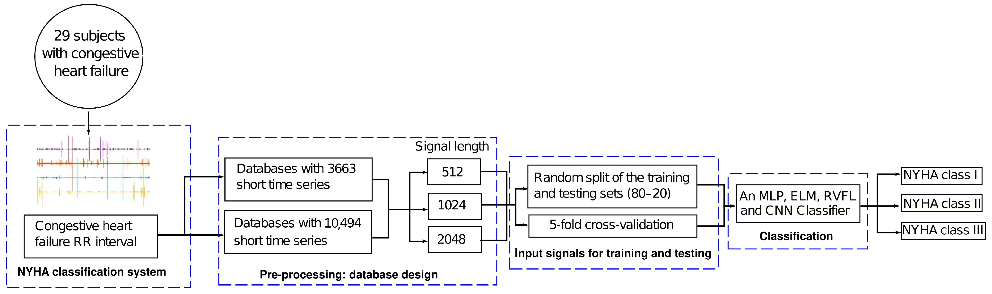
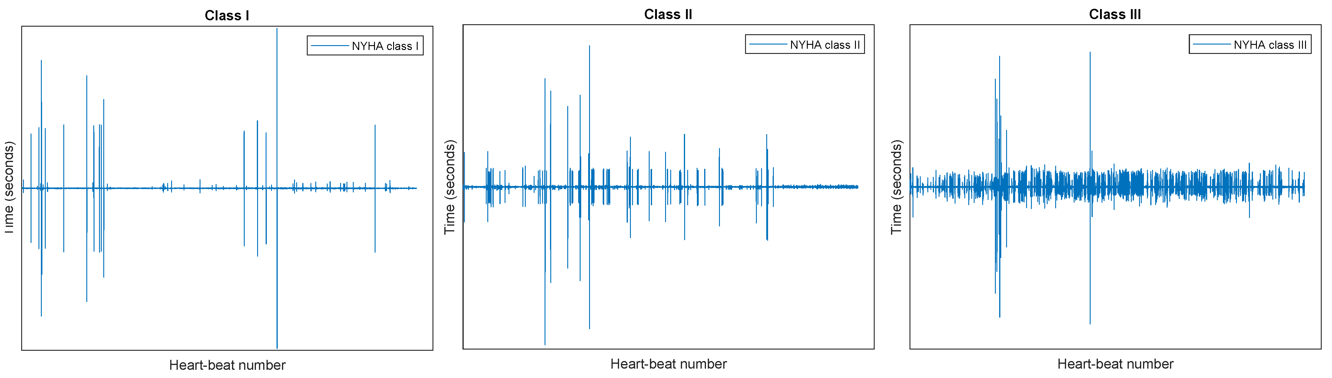
3.1. Congestive Heart Failure

The New York Heart Association (NYHA) Classification system is a widely utilized tool in the medical field. It categorizes patients who have heart failure into one of four classes based on the extent of their symptoms during rest and physical activity. In the initial stages of heart failure, the heart typically functions adequately both at rest and during activity. As the disease progresses, the heart’s capacity to meet the body’s demands during physical exertion diminishes, leading to the onset of clinical signs and symptoms during activity. As the disease advances further, patients may experience signs and symptoms of heart failure even when they are at rest.
Physicians commonly rely on the NYHA Classification system for predicting outcomes and assessing the effectiveness of treatment interventions for heart failure [63]. The classification comprises four classes, labeled I to IV, where Class I indicates milder symptoms and higher-class numbers correspond to more severe symptoms. Patients self-report their signs and symptoms, and their classification may change, either improving or worsening, depending on the severity of their condition at a given time. For a detailed breakdown of the classes, please refer to Table 1.

3.2. Selection and Preprocessing of RR Intervals

As mentioned earlier, the study of RR interval short time series has a twofold interest because most of the records for RR time series are short, and, on the long series the dynamics may change with time, requiring the analysis of short pieces to obtain insight into this process. We worked with information extracted from the Physionet.org [64], a web-based resource designed to support current research and stimulate new investigations in studying complex physiologic and clinical data.
In this research, we have selected three groups corresponding to congestive heart failure (CHF), which were freely accessed on 1 August 2023 from https://physionet.org/content/chf2db/1.0.0/ (see Table 2 for more details). Each time series is a 24 h record with a sampled frequency of 128 Hz, which was cleaned as follows:
  • Consider a finite time series y ( j ) of length N, where j = 1 , …, N;
  • Progressing from j = 3 to j = N 2 , the s value is calculated as
    s = y ( j 2 ) + y ( j 1 ) + y ( j + 1 ) + y ( j + 2 ) 4 ;
  • If y ( j ) satisfies the following condition:
    s ( 1 + w ) > y ( j ) > s ( 1 w )
    the y ( j ) value is accepted; otherwise, it is deleted ( w = 0.2 );
  • Finally, compute the new time series x ( i ) as
    x ( i ) = y ( j ) < y > σ y ( j )
Following from each 24 h record, short time series of lengths 512, 1024, and 2048 were extracted. These short series were grouped into two databases with 3663 and 10,494 records for each respective length. Subsequently, the records were grouped into classes according to the NYHA classification system (see Table 1). To train our neural network and be able to know if it is working well, let us separate the data set (see Table 2) into a training set (train) and test set (test) in a ratio of “80-20”. For this, we took random samples not in sequence (if not mixed). Also adopted was the five-fold cross-validation scheme for training and testing, a classical generalization tool in machine learning. Figure 2 shows some signals corresponding to CHF for each class in the database.

3.3. Environment

The experiments were run on a LAPTOP—CK96L4FB with Windows 11 Home Single Language 64-bit operating system, Intel(R) Core(TM) i5-10300H CPU @ 2.50 GHz 2.50 GHz, 4 cores, 8 logical processors, and 8 GB RAM. The implementation of all models was carried out in MATLAB R2020a programming language using custom scripts.

3.4. Performance Metrics

To evaluate the performance of the proposed approach in the classification of cardiovascular diseases on the test set, we applied some performance criteria that are commonly used in machine learning, namely, Accuracy (Acc), Sensitivity (Sen), Specificity (Spe), and Positive Predictive Value (PPV). These metrics are defined as follows:
A c c u r a c y = T P + T N T P + T N + F P + F N
S e n s i t i v i t y = T P T P + F N
S p e c i f i c i t y = T N F P + T N
P P V = T P T P + F P  
where the acronyms in the above equations denote the true positive ( T P ), false positive ( F P ), true negative ( T N ), and false negative rates ( F N ).

3.5. Fuzzy Activation Function

In automatic learning, the shape of the fuzzy activation function plays a fundamental role in the accuracy of the model. This function is defined as follows [65]:
φ ( x ) = 0 , x a 2 α 1 x a b a α , a x a + b 2 1 2 α 1 x a b a α , a + b 2 x b 1 , x b
Through a basic analysis, the α parameter controls the gradient of the fuzzy function. Following the experimental results discussed in [65], the neural network obtained better error rates when α = 2 . For this reason, α = 2 was the optimal value considered in the experiments in our study. More details of the fuzzy function can be found in [65].

4. Results and Discussion

In this section, we use congestive heart failure signals to conduct a series of experiments to evaluate the performance of the proposed neural network-based models. Initially, the tests were performed with a simple architecture: MLP, ELM, or RVFL. Then, the classical CNN architecture was adapted to our cardiovascular disease classification problem. The efficiency of deep feature learning for image classification [58] motivated the use of the CNN method.

4.1. Selection of Learning Models Based on Neural Networks

  • ELM and RVFL networks: These two non-iterative architectures learned nonlinear features thanks to the sigmoid function φ ( z ) = 1 / ( 1 exp ( z ) ) , chosen for its efficiency in this class of algorithms [56,66]. The random weights and biases in the hidden layer followed a uniform distribution in the [ 1 , 1 ] range [55]. In the training phase, the { 10 10 , 10 9 , , 10 9 , 10 10 } and { 500 , 700 , 900 , , 10,000 } grids were considered to estimate the optimal values of C (regularization constant) and L (hidden neurons), respectively. Table 3 shows the optimal value of the hyperparameters after an exhaustive search. It is worth mentioning that the same idea was configured for each database designed in this study;
  • MLP Network: Table 3 also includes the best MLP model for each database, choosing hyperparameters through an empirical or manual setup. We adopted this fast training phase because some experiments showed non-significant differences between a fine and empirical fit. The over-fitting problem was controlled by adding the 2 -norm to the cost function in Equation (1). The Adam optimizer was the training algorithm, and the ReLU function produced the non-linear feature learning;
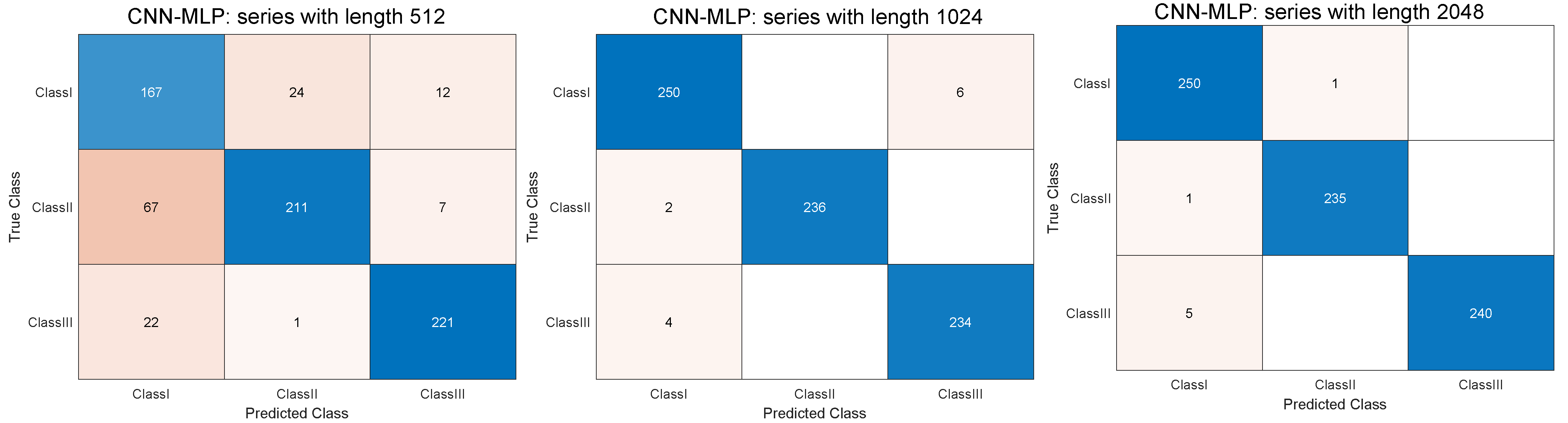
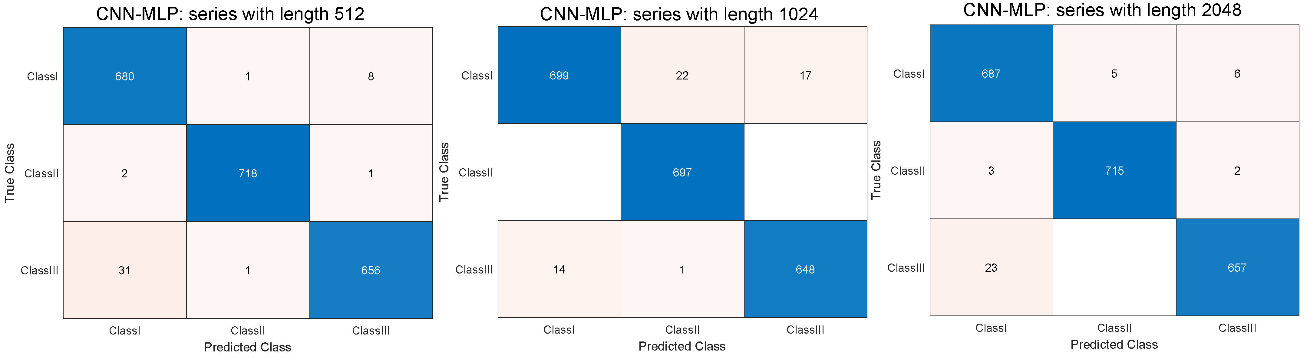
  • CNN approach: To achieve more stable results in the classification phase of cardiovascular disease, we focused on a CNN model for high-level feature extraction. The optimal feature representation can be obtained by adding convolutional layers to the CNN. Our research proposes a CNN model with seven convolutional layers, each followed by a pooling layer. The output of each of the convolutional layers was batch-normalized, and then the method learned non-linear features through the ReLU function. Finally, we concatenated a fully connected MLP with an additional convolutional layer for the final classification of the model. In the fully connected layer, the loss function considered was the crossentropyex function for the three mutually exclusive classes of congestive heart failure. The CNN network was trained with the SGDM (Stochastic Gradient Descent with Momentum) algorithm. Table 4 presents the optimal hyperparameters considered, while Table 5 shows the topology of the proposed CNN model. In this deep learning approach, both topology and hyperparameters were hand-picked to speed up the training stage. The term “padding same” in the convolutional layer indicates that the output dimension does not change with respect to the input after applying a filter or kernel.
    To explore the extraction of deep features, experimental tests were conducted by linking some feature maps with an RVFL architecture. Specifically, the inputs of the RVFL network were the outputs of the layers: pooling 3, pooling 4, pooling 5, pooling 6, and pooling 7. We named these models according to the pooling layer, such as CNN-,RVFL3, CNN-,RVFL4, CNN-,RVFL5, CNN-,RVFL6, and CNN-,RVFL7. In addition, we decided to run several training stages by assigning the epochs a number. In this experimental breakdown, the fuzzy function replaces the sigmoid function for the non-linear feature mapping, with C and L estimated manually in Table 4;
  • Five-fold cross-validation scheme: In order to corroborate the performance of the models discussed above, some experiments were repeated using the five-fold cross-validation technique of machine learning. This training and testing strategy does not consider fixed parts of the dataset, an important condition to achieve unbiased and precise evaluation metrics. In fact, the short time series were distributed over five folds (each fold with 20% of the database). Each fold was used as a test set, while the four folds remaining were used for training. For each designed database, the overall results were the average of the five runs. In view of the poor learning of the non-iterative and MLP models in cardiovascular classification, the next section includes some results of the CNN approach. To compare the performance of the CNN learning system without cross-validation, the experiments inherited the setup included in Table 4 and Table 5.

4.2. Accuracy Analysis for the Classification of Cardiovascular Diseases

With the length and number of short time series introduced in Table 2, we organized the experimental results on cardiovascular disease into two scenarios. The first corresponds to the 3663 short time series, while the second is within the 10,494 signals; each scenario is classified according to the length or size of the time series (512, 1024, and 2048). Table 6 presents the classification results for the MLP network and the non-iterative schemes—ELM and RVFL. As can be observed, all classical models considered do not achieve good testing accuracy in the classification of patients with congestive heart failure. Both ELM and RVFL achieved better accuracy rates than MLP, with a maximum value of 54%.
In search of the model that best identifies the patient’s diagnosis, we present below the expected performance of the proposed CNN approach in the classification of cardiovascular diseases (review the CNN topology and estimated optimal values in Table 3 and Table 5). Table 7 shows the overall classification performance of the deep learning models: CNN–MLP, CNN–RVFL3, CNN–RVFL4, CNN–RVFL5, CNN–RVFL6, and CNN–RVFL7. CNN–MLP is the coupled model between the convolutional layer 8 and the MLP algorithm, and the others are the ones introduced above. Clearly, deep feature extraction improves the robustness of the congestive heart failure classification process. Experimental testing results achieve a maximum accuracy of around 98% to 99%. In both scenarios considered, the models predict higher diagnostic accuracy for longer time series. The learning approaches converge (Maximum Accuracy Rate) with 64 epochs in the first scenario and 32 epochs in the second scenario. As for CCN–RVFL models, it can be seen that all the accuracy results in the configured databases improve according to the depth of the feature map, which is an important analysis for the final decision of the number of convolutional layers in deep feature learning. Comparing the performance with MLP, ELM, and RVFL (see Table 6), the proposed CNN approach clearly improves the diagnosis of cardiovascular diseases.
The confusion matrix for the CNN–MLP model within the three categories of congestive heart failure is shown in Figure 3 and Figure 4. In these experimental results, the number of epochs in the two scenarios designed was 64 and 30, respectively. With the TP, FP, TN, and FN rates for each confusion matrix, the performance metrics for every scenario and class are reflected in Table 8. In the case of signals with length 2048 in the first scenario, for class I signals, it can be noted that 0.39% of signals are misclassified as class II. In addition, 0.42% of class II signals are misclassified as class I signals. Further, approximately 2.08% of class III signals are wrongly labeled as class I signals. The confusion matrices with lower performance over signals with lengths 512 and 1024 can be interpreted similarly. Focusing now on the second scenario, similar to the first scenario, the CNN–MLP model achieved better results for the series with length 2048. In this case, 0.70% of the class I signals are wrongly labeled as class II, and 0.84% are wrongly classified as class III. For class II, 0.42% and 0.28% are wrongly labeled as class I and class III, respectively. Furthermore, for class III signals, it can be seen that 3.46% of signals are wrongly labeled as class I. Additionally, 98.14% of the signals of length 2048 are correctly classified.
From a clinical viewpoint, patients in class I who are misclassified will attract unnecessary attention since the cardiovascular disease is mild or moderate. However, time series incorrectly labeled in classes II and III may cause more serious consequences, such as delayed treatment. In this experiment, associated with the confusion matrices discussed in the previous paragraph, 0.42% and 2.08% of the time series in classes II and III are wrongly classified as another, respectively. In the second scenario, 0.42% of class II series are misclassified, and 2.08% of class III series or signals are mislabeled. The Acc PPV, Sen, and Spe performance metrics for all confusion matrices can be reviewed in Table 8.
  • Performance of CNN for five-fold cross-validation: Here, the paper details the generalization ability of CNN in Table 9 and Table 10 under the five-fold cross-validation criterion. As before, 64 and 32 were the number of epochs considered for the first and second scenario databases, respectively. The classification of cardiovascular disease with this training and testing rule was comparable with the scheme without cross-validation (see Table 7 and Table 8). The random initialization of parameters (weights and biases) and the average value of the five runs explain the bounded variation between evaluation metrics. This proves the performance of the proposed CNN method and the importance of deep feature extraction in the final model decision.
In conclusion, the current study tackles a classification problem for cardiovascular diseases using neural networks. The methods with vector inputs—MLP, ELM, and RVFL—did not satisfactorily classify the three classes of congestive heart failure; ELM and RVFL achieved a higher accuracy rate of 54%. Adapting tensor inputs in a CNN structure with eight convolutional layers significantly improved the learning of features for medical diagnosis. The accuracy of the model was evaluated according to the depth of the feature map, coupled separately with the RVFL network for the final classification. The analysis showed that the CNN framework successfully classified the three classes of cardiovascular disease with an accuracy of 98% and 99%. As expected, the classification of the model is more robust in terms of the length of the short time series. The CNN model repeated a similar behavior with the cross-validation scheme.
The extraction of deep abstract features through convolutional filters is a possible explanation for the better performance of the proposed CNN approach. Without human intervention, the learning system captures important information from the input time series and forms a meaningful representation of the data by combining low-level features. The system could be installed in a low-cost medical electronic device and serve as a preliminary diagnostic tool in health centers where access to a cardiologist is difficult. The results could be sent to a cardiology expert in a clinic or hospital through the internet to minimize the diagnostic time and reduce the number of misdiagnoses.

4.3. Limitations and Recommendations for Further Research

The cases of cardiovascular disease reported every year are numerous, and the use of neural networks to diagnose this disease can ease this burden. It could also improve the efficiency of healthcare systems. Even laypeople can understand their physical situation and detect this disease at an early stage. It may be seen as a preventive method to stop the disease from becoming worse. Nevertheless, there are also some limitations to this paper, discussed below:
  • The diagnosis of complex cardiac diseases may require more features to achieve acceptable results. Considering the CNN classifier and the other conventional methods employed, the processing time increases with the length of the time series;
  • The performance of the CNN approach is affected by the number of features used in the short time series, addressed in the literature as an additional hyperparameter by trial and error. This may introduce a certain degree of arbitrariness in the final classification of the model;
  • The samples classified according to the length of the time series used in the experiments come from a single institution. It could be desirable to validate the model with other open-access databases.
In a future study, we aim to explore RR-interval time series in other applications that may be of interest to humankind, that is, through learning models, to detect types of heart disease and categorize their level of disease (mild or major). Another proposal will be to carefully investigate and discuss the impact of some parameters on the performance of the proposed approach. The approach presented here will facilitate the implementation of more complex models to improve performance as well as test the results with larger databases.

5. Conclusions

Cardiovascular disease leads to a high mortality rate worldwide, and the use of machine learning tools can help prevent this disease by identifying people with high cardiovascular risk. Thus, this research explores the use of three classical variants of neural networks to classify three groups of patients with CHF. Precisely, the study considered the iterative method MLP, two non-iterative models (ELM and RVFL), and the CNN approach. Through a series of experiments, the results showed that the deep feature learning system obtained better classification rates than MLP, ELM, and RVFL. Several scenarios designed by coupling some deep feature maps with the RVFL model showed very high simulation accuracy. The overall accuracy rate of CNN–MLP and CNN–RVFL varies between 98% and 99%, relevant models with very good sensitivity and specificity. On the other hand, the MLP, ELM, and RVFL methods did not learn relevant features from the data, leading to unreliable classification rates.

Author Contributions

Conceptualization, J.L.L. and J.A.V.-C.; methodology, J.L.L. and J.A.V.-C.; software, J.A.V.-C.; experimental execution and validation, J.L.L. and J.A.V.-C.; research, J.L.L. and J.A.V.-C.; writing—original draft preparation, J.L.L. and J.A.V.-C.; writing—review and editing, J.L.L.; visualization, J.L.L.; supervision, J.L.L.; project administration, J.L.L.; funding acquisition, J.L.L. All authors have read and agreed to the published version of the manuscript.

Funding

This research was funded by project grants “Fondecyt 11230276” (J. L. López) from the National Agency for Research and Development (ANID) of the Chilean government.

Institutional Review Board Statement

Not applicable.

Informed Consent Statement

Not applicable.

Data Availability Statement

The developed codes for this research are available at https://github.com/jlophys and can be downloaded freely. Any questions regarding the codes can be directed to the corresponding author.

Acknowledgments

The authors acknowledge CIIA for permitting the use of their facilities as well as Luis Morán for their technical assistance and Viviana Torres for administrative support.

Conflicts of Interest

The authors declare no conflict of interest. The funders had no role in the design of the study; in the collection, analyses, or interpretation of data; in the writing of the manuscript; or in the decision to publish the results.

Abbreviations

The following abbreviations are used in this manuscript:
MLPMultilayer Perceptron
ELMExtreme Learning Machine
RVFLRandom Vector Functional Link
CNNConvolutional Neural Network
ReLURectified Linear Unit
PPVPositive Predictive Value
TPTrue Positive
FPFalse Positive
TNTrue Negative
FNFalse Negative
SGDMStochastic Gradient Descent with Momentum
CHFCongestive Heart Failure
NYHANew York Heart Association
HRVHeart Rate Variability
ECGElectrocardiogram
EMDEmpirical Mode Decomposition
DWTDiscrete Wavelet Transform
MFDFAMultifractal Detrended Fluctuation Analysis
DFADetrended Fluctuation Analysis
WTWavelet Analysis

References

  1. Glass, L.; Hunter, P. There is a theory of heart. Phys. D Nonlinear Phenom. 1990, 43, 1–16. [Google Scholar] [CrossRef]
  2. Malik, M. Heart rate variability: Standards of measurement, physiological interpretation, and clinical use: Task force of the European Society of Cardiology and the North American Society for Pacing and Electrophysiology. Ann. Noninvasive Electrocardiol. 1996, 1, 151–181. [Google Scholar] [CrossRef]
  3. Sung, C.W.; Shieh, J.S.; Chang, W.T.; Lee, Y.W.; Lyu, J.H.; Ong, H.N.; Chen, W.T.; Huang, C.H.; Chen, W.J.; Jaw, F.S. Machine learning analysis of heart rate variability for the detection of seizures in comatose cardiac arrest survivors. IEEE Access 2020, 8, 160515–160525. [Google Scholar] [CrossRef]
  4. Chiew, C.J.; Liu, N.; Tagami, T.; Wong, T.H.; Koh, Z.X.; Ong, M.E. Heart rate variability based machine learning models for risk prediction of suspected sepsis patients in the emergency department. Medicine 2019, 98, e14197. [Google Scholar] [CrossRef]
  5. Agliari, E.; Barra, A.; Barra, O.A.; Fachechi, A.; Franceschi Vento, L.; Moretti, L. Detecting cardiac pathologies via machine learning on heart-rate variability time series and related markers. Sci. Rep. 2020, 10, 8845. [Google Scholar] [CrossRef]
  6. Miglis, M. Chapter 12 - Sleep and the Autonomic Nervous System. In Sleep and Neurologic Disease; Miglis, M.G., Ed.; Academic Press: San Diego, CA, USA, 2017; pp. 227–244. [Google Scholar] [CrossRef]
  7. Chapter 27-Ambulatory Electrocardiography. In Chou’s Electrocardiography in Clinical Practice, 6th ed.; Surawicz, B.; Knilans, T.K. (Eds.) W.B. Saunders: Philadelphia, PA, USA, 2008; pp. 631–645. [Google Scholar] [CrossRef]
  8. Bak, P.; Tang, C.; Wiesenfeld, K. Self-Organized Criticality. Phys. Rev. A 1988, 38, 364–374. [Google Scholar] [CrossRef]
  9. Lin, D. Robustness and perturbation in the modeled cascade heart rate variability. Phys. Rev. E. Stat. Nonlinear Soft Matter Phys. 2003, 67, 031914. [Google Scholar] [CrossRef]
  10. Kiyono, K.; Struzik, Z.; Aoyagi, N.; Sakata, S.; Hayano, J.; Yamamoto, Y. Critical Scale Invariance in a Healthy Human Heart Rate. Phys. Rev. Lett. 2004, 93, 178103. [Google Scholar] [CrossRef]
  11. Kotani, K.; Struzik, Z.; Takamasu, K.; Stanley, H.; Yamamoto, Y. Model for complex heart rate dynamics in health and diseases. Phys. Rev. E Stat. Nonlinear Soft Matter Phys. 2005, 72, 041904. [Google Scholar] [CrossRef]
  12. Makowiec, D.; Galaska, R.; Dudkowska, A.; Rynkiewicz, A.; Zwierz, M. Long-range dependencies in heart rate signals—Revisited. Phys. A Stat. Mech. Its Appl. 2006, 369, 632–644. [Google Scholar] [CrossRef]
  13. Makowiec, D.; Dudkowska, A.; Galaska, R.; Rynkiewicz, A. Multifractal estimates of monofractality in RR-heart series in power spectrum ranges. Phys. A Stat. Mech. Its Appl. 2009, 388, 3486–3502. [Google Scholar] [CrossRef]
  14. Makowiec, D.; Rynkiewicz, A.; Galaska, R.; Wdowczyk, J.; Zarczynska-Buchowiecka, M. Reading multifractal spectra: Aging by multifractal analysis of heart rate. Epl (Europhys. Lett.) 2011, 94, 68005. [Google Scholar] [CrossRef]
  15. Hadase, M.; Azuma, A.; Zen, K.; Asada, S.; Kawasaki, T.; Kamitani, T.; Kawasaki, S.; Sugihara, H.; Matsubara, H. Very Low Frequency Power of Heart Rate Variability is a Powerful Predictor of Clinical Prognosis in Patients with Congestive Heart Failure. Circ. J. 2004, 68, 343–347. [Google Scholar] [CrossRef]
  16. Usui, H.; Nishida, Y. The very low-frequency band of heart rate variability represents the slow recovery component after a mental stress task. PLoS ONE 2017, 12, e0182611. [Google Scholar] [CrossRef]
  17. Serrador, J.M.; Finlayson, H.C.; Hughson, R.L. Physical activity is a major contributor to the ultra low frequency components of heart rate variability. Heart (Br. Card. Soc.) 1999, 82. [Google Scholar] [CrossRef]
  18. Rodríguez-Liñares, L.; Lado, M.; Vila, X.; Méndez, A.; Cuesta, P. gHRV: Heart Rate Variability analysis made easy. Comput. Methods Programs Biomed. 2014, 116, 26–38. [Google Scholar] [CrossRef]
  19. Flevari, K.; Vagiakis, E.; Zakynthinos, S. Heart rate variability is augmented in patients with positional obstructive sleep apnea, but only supine LF/HF index correlates with its severity. Sleep Breath. 2014, 19, 359–367. [Google Scholar] [CrossRef]
  20. Ebrahimi, F.; Setarehdan, S.K.; Ayala-Moyeda, J.; Nazeran, H. Automatic sleep staging using empirical mode decomposition, discrete wavelet transform, time-domain, and nonlinear dynamics features of heart rate variability signals. Comput. Methods Programs Biomed. 2013, 112, 47–57. [Google Scholar] [CrossRef]
  21. Nayak, S.K.; Jarzębski, M.; Gramza-Michałowska, A.; Pal, K. Automated Detection of Cannabis-Induced Alteration in Cardiac Autonomic Regulation of the Indian Paddy-Field Workers Using Empirical Mode Decomposition, Discrete Wavelet Transform and Wavelet Packet Decomposition Techniques with HRV Signals. Appl. Sci. 2022, 12, 10371. [Google Scholar] [CrossRef]
  22. Lee, K.H.; Byun, S. Age Prediction in Healthy Subjects Using RR Intervals and Heart Rate Variability: A Pilot Study Based on Deep Learning. Appl. Sci. 2023, 13, 2932. [Google Scholar] [CrossRef]
  23. Eltahir, M.M.; Hussain, L.; Malibari, A.A.; K. Nour, M.; Obayya, M.; Mohsen, H.; Yousif, A.; Ahmed Hamza, M. A Bayesian dynamic inference approach based on extracted gray level co-occurrence (GLCM) features for the dynamical analysis of congestive heart failure. Appl. Sci. 2022, 12, 6350. [Google Scholar] [CrossRef]
  24. Zhang, Y.; Wei, S.; Zhang, L.; Liu, C. Comparing the Performance of Random Forest, SVM and Their Variants for ECG Quality Assessment Combined with Nonlinear Features. J. Med. Biol. Eng. 2018, 39, 381–392. [Google Scholar] [CrossRef]
  25. Karpagachelvi, S.; Arthanari, M.; Sivakumar, M. Classification of electrocardiogram signals with support vector machines and extreme learning machine. Neural Comput. Appl. 2012, 21, 1331–1339. [Google Scholar] [CrossRef]
  26. Zhou, X.; Zhu, X.; Nakamura, K.; Noro, M. Electrocardiogram quality assessment with a generalized deep learning model assisted by conditional generative adversarial networks. Life 2021, 11, 1013. [Google Scholar] [CrossRef]
  27. Hannun, A.Y.; Rajpurkar, P.; Haghpanahi, M.; Tison, G.H.; Bourn, C.; Turakhia, M.P.; Ng, A.Y. Cardiologist-level arrhythmia detection and classification in ambulatory electrocardiograms using a deep neural network. Nat. Med. 2019, 25, 65–69. [Google Scholar] [CrossRef]
  28. Brisk, R.; Bond, R.; Banks, E.; Piadlo, A.; Finlay, D.; McLaughlin, J.; McEneaney, D. Deep learning to automatically interpret images of the electrocardiogram: Do we need the raw samples? J. Electrocardiol. 2019, 57, S65–S69. [Google Scholar] [CrossRef]
  29. Sinnecker, D. A deep neural network trained to interpret results from electrocardiograms: Better than physicians? Lancet Digit. Health 2020, 2, e332–e333. [Google Scholar] [CrossRef]
  30. Ihsanto, E.; Ramli, K.; Sudiana, D.; Gunawan, T.S. Fast and accurate algorithm for ECG authentication using residual depthwise separable convolutional neural networks. Appl. Sci. 2020, 10, 3304. [Google Scholar] [CrossRef]
  31. Naeem, S.; Ali, A.; Qadri, S.; Khan Mashwani, W.; Tairan, N.; Shah, H.; Fayaz, M.; Jamal, F.; Chesneau, C.; Anam, S. Machine-learning based hybrid-feature analysis for liver cancer classification using fused (MR and CT) images. Appl. Sci. 2020, 10, 3134. [Google Scholar] [CrossRef]
  32. Yan, H.; Jiang, Y.; Zheng, J.; Peng, C.; Li, Q. A multilayer perceptron-based medical decision support system for heart disease diagnosis. Expert Syst. Appl. 2006, 30, 272–281. [Google Scholar] [CrossRef]
  33. Gupta, P.; Seth, D. Early Detection of Heart Disease Using Multilayer Perceptron. In Micro-Electronics and Telecommunication Engineering: Proceedings of 6th ICMETE 2022; Springer Nature: Singapore, 2023; pp. 309–315. [Google Scholar]
  34. He, W.; Xie, Y.; Lu, H.; Wang, M.; Chen, H. Predicting coronary atherosclerotic heart disease: An extreme learning machine with improved salp swarm algorithm. Symmetry 2020, 12, 1651. [Google Scholar] [CrossRef]
  35. Saputra, D.C.E.; Sunat, K.; Ratnaningsih, T. A new artificial intelligence approach using extreme learning machine as the potentially effective model to predict and analyze the diagnosis of anemia. Healthcare 2023, 11, 697. [Google Scholar] [CrossRef] [PubMed]
  36. Flores, J.; Loaeza, R.; Rodriguez Rangel, H.; González-santoyo, F.; Romero, B.; Gómez, A. Financial Time Series Forecasting Using a Hybrid Neural Evolutive Approach. In Proceedings of the the XV SIGEF International Conference, Lugo, Spain, 3–8 October 2009. [Google Scholar]
  37. Alba, E.; Mendoza, M. Bayesian Forecasting Methods for Short Time Series. Foresight Int. J. Appl. Forecast. 2007, 8, 41–44. [Google Scholar]
  38. Ernst, J.; Nau, G.; Bar-Joseph, Z. Clustering Short Time Series Gene Expression Data. Bioinformatics 2005, 21 (Suppl. S1), i159–i168. [Google Scholar] [CrossRef]
  39. López, J.L.; Contreras, J.G. Performance of multifractal detrended fluctuation analysis on short time series. Phys. Rev. E 2013, 87, 022918. [Google Scholar] [CrossRef]
  40. López, J.; Hernández, S.; Urrutia, A.; López-Cortés, X.; Araya, H.; Morales-Salinas, L. Effect of missing data on short time series and their application in the characterization of surface temperature by detrended fluctuation analysis. Comput. Geosci. 2021, 153, 104794. [Google Scholar] [CrossRef]
  41. Kleiger, R.E.; Stein, P.K.; Bosner, M.S.; Rottman, J.N. Time domain measurements of heart rate variability. Cardiol. Clin. 1992, 10, 487–498. [Google Scholar] [CrossRef]
  42. The Look AHEAD Research Group. Long-term effects of a lifestyle intervention on weight and cardiovascular risk factors in individuals with type 2 diabetes mellitus: Four-year results of the Look AHEAD trial. Arch. Intern. Med. 2010, 170, 1566–1575. [Google Scholar]
  43. Wang, T.; Lu, C.; Sun, Y.; Yang, M.; Liu, C.; Ou, C. Automatic ECG classification using continuous wavelet transform and convolutional neural network. Entropy 2021, 23, 119. [Google Scholar] [CrossRef]
  44. Rahul, J.; Sora, M.; Sharma, L.D.; Bohat, V.K. An improved cardiac arrhythmia classification using an RR interval-based approach. Biocybern. Biomed. Eng. 2021, 41, 656–666. [Google Scholar] [CrossRef]
  45. Faust, O.; Kareem, M.; Ali, A.; Ciaccio, E.J.; Acharya, U.R. Automated arrhythmia detection based on RR intervals. Diagnostics 2021, 11, 1446. [Google Scholar] [CrossRef] [PubMed]
  46. Heidari, A.A.; Faris, H.; Mirjalili, S.; Aljarah, I.; Mafarja, M. Ant lion optimizer: Theory, literature review, and application in multi-layer perceptron neural networks. Nat.-Inspired Optim. Theor. Lit. Rev. Appl. 2020, 811, 23–46. [Google Scholar]
  47. Afzal, S.; Ziapour, B.M.; Shokri, A.; Shakibi, H.; Sobhani, B. Building energy consumption prediction using multilayer perceptron neural network-assisted models; comparison of different optimization algorithms. Energy 2023, 282, 128446. [Google Scholar] [CrossRef]
  48. Lima-Junior, F.R.; Carpinetti, L.C.R. Predicting supply chain performance based on SCOR® metrics and multilayer perceptron neural networks. Int. J. Prod. Econ. 2019, 212, 19–38. [Google Scholar] [CrossRef]
  49. Wijnhoven, R.G.; de With, P. Fast training of object detection using stochastic gradient descent. In Proceedings of the 2010 20th International Conference on Pattern Recognition, Istanbul, Turkey, 23–26 August 2010; pp. 424–427. [Google Scholar]
  50. Übeyli, E.D. Combined neural network model employing wavelet coefficients for EEG signals classification. Digit. Signal Process. 2009, 19, 297–308. [Google Scholar] [CrossRef]
  51. Pao, Y.H.; Phillips, S.M.; Sobajic, D.J. Neural-net computing and the intelligent control of systems. Int. J. Control. 1992, 56, 263–289. [Google Scholar] [CrossRef]
  52. Zhang, L.; Suganthan, P.N. A comprehensive evaluation of random vector functional link networks. Inf. Sci. 2016, 367, 1094–1105. [Google Scholar] [CrossRef]
  53. Rao, C.R.; Mitra, S.K. Further contributions to the theory of generalized inverse of matrices and its applications. Sankhyā Indian J. Stat. Ser. A 1971, 33, 289–300. [Google Scholar]
  54. Malik, A.; Gao, R.; Ganaie, M.; Tanveer, M.; Suganthan, P.N. Random vector functional link network: Recent developments, applications, and future directions. Appl. Soft Comput. 2023, 143, 110377. [Google Scholar] [CrossRef]
  55. Huang, G.B.; Zhu, Q.Y.; Siew, C.K. Extreme learning machine: Theory and applications. Neurocomputing 2006, 70, 489–501. [Google Scholar] [CrossRef]
  56. Vásquez-Coronel, J.A.; Mora, M.; Vilches, K. A Review of multilayer extreme learning machine neural networks. Artif. Intell. Rev. 2023, 19, 1–52. [Google Scholar] [CrossRef]
  57. Bhatt, D.; Patel, C.; Talsania, H.; Patel, J.; Vaghela, R.; Pandya, S.; Modi, K.; Ghayvat, H. CNN variants for computer vision: History, architecture, application, challenges and future scope. Electronics 2021, 10, 2470. [Google Scholar] [CrossRef]
  58. Khanday, N.Y.; Sofi, S.A. Deep insight: Convolutional neural network and its applications for COVID-19 prognosis. Biomed. Signal Process. Control. 2021, 69, 102814. [Google Scholar] [CrossRef] [PubMed]
  59. Boureau, Y.L.; Ponce, J.; LeCun, Y. A theoretical analysis of feature pooling in visual recognition. In Proceedings of the International Conference on Machine Learning (ICML), Haifa, Israel, 21–24 June 2010; pp. 111–118. [Google Scholar]
  60. Wang, T.; Wu, D.J.; Coates, A.; Ng, A.Y. End-to-end text recognition with convolutional neural networks. In Proceedings of the International Conference on Pattern Recognition (ICPR), Tsukuba, Japan, 11–15 November 2012; pp. 3304–3308. [Google Scholar]
  61. Zeiler, M.D.; Fergus, R. Visualizing and understanding convolutional networks. In Proceedings of the Computer Vision–ECCV 2014: 13th European Conference, Zurich, Switzerland, 6–12 September 2014; Proceedings, Part I 13. 2014; pp. 818–833. [Google Scholar]
  62. Russakovsky, O.; Deng, J.; Su, H.; Krause, J.; Satheesh, S.; Ma, S.; Huang, Z.; Karpathy, A.; Khosla, A.; Bernstein, M.; et al. Imagenet large scale visual recognition challenge. Int. J. Comput. Vis. 2015, 115, 211–252. [Google Scholar] [CrossRef]
  63. Cameron, M.H. Physical Rehabilitation; W.B. Saunders: Saint Louis, MI, USA, 2007. [Google Scholar] [CrossRef]
  64. Goldberger, A.L.; Amaral, L.A.N.; Glass, L.; Hausdorff, J.M.; Ivanov, P.C.; Mark, R.G.; Mietus, J.E.; Moody, G.B.; Peng, C.K.; Stanley, H.E. PhysioBank, PhysioToolkit, and PhysioNet: Components of a New Research Resource for Complex Physiologic Signals. Circulation 2000, 101, 215–220. [Google Scholar] [CrossRef]
  65. Goel, T.; Nehra, V.; Vishwakarma, V.P. An adaptive non-symmetric fuzzy activation function-based extreme learning machines for face recognition. Arab. J. Sci. Eng. 2017, 42, 805–816. [Google Scholar] [CrossRef]
  66. Liu, X.; Xu, L. The universal consistency of extreme learning machine. Neurocomputing 2018, 311, 176–182. [Google Scholar] [CrossRef]
Figure 1. Block diagram of the proposed methodology for the classification of heart disease.
Applsci 13 13211 g001
Figure 2. Examples of heart time series for three different classes: each plot illustrates the first 7680 heartbeats with their corresponding RR interval for the three classes considered.
Applsci 13 13211 g002
Figure 3. Confusion matrices of three classes for cardiovascular diseases within the first scenario and performance of CNN–MLP.
Applsci 13 13211 g003
Figure 4. Confusion matrices of three classes for cardiovascular diseases within the second scenario and performance of CNN–MLP.
Applsci 13 13211 g004
Table 1. Congestive heart failure categories.
ClassLimitationDescription
NYHA IRelativePatients that have no limitation to physical activity.
NYHA IIRelativePatients with cardiac disease that results in slight limitation to physical activity, with symptoms such as fatigue, palpations, dyspnea, or angina pain.
NYHA IIIAbsolutePatients with cardiac disease who are comfortable at rest; however, less-than-ordinary activity causes fatigue, palpation, dyspnea, or angina pain.
NYHA IVAbsolutePatients with cardiac disease that results in the inability to carry out any physical activity.
Table 2. Databases for cardiovascular diseases.
Database NameDescriptionNumber of Subjects StudiedNumber of Short Time SeriesLength of Short Time Series
Congestive Heart Failure RR IntervalBeat annotation files (about 24 h each) from 29 subjects with congestive heart failure (NYHA classes I, II, and III)293663, 10,494512, 1024, 2048
Table 3. Estimated hyperparameters: ELM, RVFL, and MLP.
ScenariosSignal LengthHyperparameter
MLPELMRVFL
First scenario: databases with 3663 samples512Cross-entropy loss, ReLU activation, 64 mini-batches, a learning rate of 5 × 10 4 , 2 -regularization of 10 8 , Adam optimizer, 50 epochs, and three hidden layers (50, 100, and 40 neurons).sigmoid activation, C = 0.1 , L = 8700 .sigmoid activation, C = 1 , L = 4900 .
1024MLP model within 512 with a learning rate of 5 × 10 3 and three hidden layers (100, 100, and 40 neurons).sigmoid activation, C = 0.01 , L = 7300 .sigmoid activation, C = 0.1 , L = 9300 .
2048MLP model within 512 with 60 epochs, 2 -regularizer of 10 20 and three hidden layers (50, 20, and 100 neurons).sigmoid activation, C = 10 3 , L = 9700 .sigmoid activation, C = 1 , L = 3300 .
Second scenario: 10,494 short time series512MLP model within 512 with 75 epochs, 2 -regularizer of 10 20 and two hidden layers (50 and 20 neurons).sigmoid activation, L = 7500 , C = 10 3 .sigmoid activation, L = 6700 , C = 10 .
1024MLP model within 512 with 75 epochs, 2 -regularizer of 10 20 and two hidden layers (50 and 20 neurons).sigmoid activation, L = 6900 , C = 0.01 .sigmoid activation, L = 6900 , C = 0.01 .
2048MLP model within 512 with 37 epochs, 2 -regularizer of 10 10 , a learning rate of 5 × 10 3 and two hidden layers (70 and 40 neurons).sigmoid activation, L = 4900 , C = 0.1 .sigmoid activation, L = 4900 , C = 0.1 .
Table 4. Hyperparameters of the proposed CNN approach.
ScenariosSignal LengthHyperparameter
CNN–MLPCNN–RVFL
First scenario and second scenario512, 1024, and 2048crossentropyex loss, ReLU activation, 64 mini-batches, a learning rate of 0.022, 0.099 as momentum, 2 -regularizer of 0.03, SGDM optimizer.Hyperparameters of the feature map and RVFL (fuzzy activation, L = 5 , and C = 0.1 ).
Table 5. Topology of the proposed CNN approach for classifying congestive heart disease.
Layer TypeFilter SizeStridePaddingActivation
Convolutional 7 × 7 × 32 1sameReLU
Max Pooling 2 × 2 2
Convolutional 5 × 5 × 64 1sameReLU
Max Pooling 2 × 2 2
Convolutional 5 × 5 × 64 1sameReLU
Max Pooling 2 × 2 2
Convolutional 5 × 5 × 64 1sameReLU
Max Pooling 2 × 2 2
Convolutional 3 × 3 × 32 1sameReLU
Max Pooling 2 × 2 2
Convolutional 3 × 3 × 32 1sameReLU
Max Pooling 2 × 2 2
Convolutional 3 × 3 × 16 1sameReLU
Max Pooling 2 × 2 2
Convolutional 3 × 3 × 32 1sameReLU
Fully connected3Softmax
Table 6. Overall accuracy of MLP, ELM, and RVFL approaches within cardiovascular diseases.
ScenariosSignal LengthOverall Accuracy (%)
MLPELMRVFL
First scenario: databases with 3663 samples51251.6453.5554.23
102450.2754.5154.10
204849.1854.6453.83
Second scenario: databases with 10,494 samples51250.5251.9150.29
102450.0550.5750.00
204850.0950.6249.71
Table 7. Overall accuracy of CNN for the classification of cardiovascular disease.
ScenariosSignal LengthEpochsOverall Accuracy (%)
CNN–MLPCNN–RVFL3CNN–RVFL4CNN–RVFL5CNN–RVFL6CNN–RVFL7
First scenario: databases with 3663 samples5128 62.30 53.69 56.83 56.69 63.52 62.30
16 69.81 56.97 60.79 68.99 71.99 70.90
32 79.78 57.79 65.98 76.78 81.28 85.66
64 81.69 62.84 70.49 75.00 82.92 83.74
10248 70.77 62.30 70.63 70.77 71.99 68.03
16 75.27 57.24 62.02 78.28 84.02 80.87
32 96.99 63.80 66.94 86.07 96.72 97.13
64 98.91 64.89 73.50 87.02 98.63 98.91
20488 80.74 61.07 62.98 60.66 71.17 80.60
16 93.58 64.48 70.08 67.35 82.51 92.21
32 97.68 67.35 75.55 77.46 89.89 96.45
64 99.04 65.57 81.01 88.66 97.54 99.18
Second scenario: databases with 10,494 samples5128 89.04 64.25 75.83 84.08 88.70 88.51
16 93.99 65.30 73.45 86.32 94.71 95.00
32 97.52 66.63 75.31 86.27 97.04 97.09
10248 89.13 59.77 69.54 79.36 80.03 81.27
16 92.09 67.54 74.88 83.94 90.85 91.13
32 97.14 71.45 82.55 91.99 97.33 97.71
20488 97.09 64.87 68.73 84.60 91.28 95.76
16 97.28 66.83 78.12 83.94 94.23 96.19
32 98.62 70.97 77.36 85.99 97.90 98.43
Table 8. Evaluation metrics of CNN–MLP for each of the confusion matrices included in Figure 3 and Figure 4.
ScenariosSignal LengthClass I (%)Class II (%)Class III (%)
AccPPVSenSpeAccPPVSenSpeAccPPVSenSpe
First scenario: databases with 3663 samples51282.9265.2382.2783.1886.4789.4174.0494.4194.2692.0890.5796.11
102498.3697.6697.6698.7499.7310099.1610098.6397.5098.3198.78
204899.0497.6699.6098.7599.7399.5899.5899.8099.3210097.96100
Second scenario: databases with 10,494 samples51297.9995.3798.6997.6699.7699.7299.5899.8698.0598.6595.3599.36
102497.4798.0494.7298.9798.9096.8110098.3698.3897.4497.7498.82
204898.2396.3598.4298.1499.4899.3199.3199.6498.5298.8096.6299.44
Table 9. Overall accuracy of CNN for five-fold cross-validation.
ScenariosSignal LengthOverall Accuracy (%)
CNN–MLPCNN–RVFL3CNN–RVFL4CNN–RVFL5CNN–RVFL6CNN–RVFL7
First scenario: databases with 3663 samples51281.9663.0969.5378.5282.5683.01
102497.5164.0172.8786.2196.1097.58
204896.0065.6674.0185.6895.1096.58
Second scenario: databases with 10,494 samples51296.3865.4476.4586.0996.7897.00
102497.1071.7383.2790.0096.7297.60
204897.9072.8784.0489.6998.3198.40
Table 10. Evaluation metrics of CCN–MLP for five-fold cross-validation.
ScenariosSignal LengthClass I (%)Class II (%)Class III (%)
AccPPVSenSpeAccPPVSenSpeAccPPVSenSpe
First scenario: databases with 3663 samples51284.2279.4971.8690.5187.6378.8286.1088.4092.0688.2288.4094.12
102497.7896.6596.9198.2399.1199.1398.1399.5998.1296.7997.5198.43
204898.1696.7198.0998.2399.8698.7599.5999.2198.2997.8596.8299.00
Second scenario: databases with 10,494 samples51296.7496.4393.7498.2098.7097.9098.1998.9697.3295.0697.1597.40
102497.3296.6195.3198.3398.8997.9198.8098.8597.9996.9497.2198.38
204897.0096.0098.0797.9499.5699.6998.9999.8498.2698.1296.6499.07
Disclaimer/Publisher’s Note: The statements, opinions and data contained in all publications are solely those of the individual author(s) and contributor(s) and not of MDPI and/or the editor(s). MDPI and/or the editor(s) disclaim responsibility for any injury to people or property resulting from any ideas, methods, instructions or products referred to in the content.

