A Comparative Study on Recent Progress of Machine Learning-Based Human Activity Recognition with Radar

Abstract

The importance of radar-based human activity recognition has increased significantly over the last two decades in safety and smart surveillance applications due to its superiority in vision-based sensing in the presence of poor environmental conditions like low illumination, increased radiative heat, occlusion, and fog. Increased public sensitivity to privacy protection and the progress of cost-effective manufacturing have led to higher acceptance and distribution of this technology. Deep learning approaches have proven that manual feature extraction that relies heavily on process knowledge can be avoided due to its hierarchical, non-descriptive nature. On the other hand, ML techniques based on manual feature extraction provide a robust, yet empirical-based approach, where the computational effort is comparatively low. This review outlines the basics of classical ML- and DL-based human activity recognition and its advances, taking the recent progress in both categories into account. For every category, state-of-the-art methods are introduced, briefly explained, and their related works summarized. A comparative study is performed to evaluate the performance and computational effort based on a benchmarking dataset to provide a common basis for the assessment of the techniques’ degrees of suitability.

1. Introduction

In the last two decades, civil radar-based applications used for human sensing and human activity recognition (HAR) have made significant progress. This has been triggered and supported by the rapid development in semiconductor technologies in recent decades, particularly the drastic changes in the concept of radar. Modern radar systems are highly integrated, i.e., the most important circuits are housed on a single chip or a small circuit board.

The potential of radar-based sensing and recognition technologies has been discovered across a variety of different scientific domains, and they have been the target of numerous previous and recent research studies. The first studies dealt with the detection and recognition of humans in indoor environments in applications related to security [1,2,3,4,5,6]. Medical applications, i.e., the monitoring of patients, extended their applicability [7,8,9,10,11,12,13] to sub-domains, e.g., vital sign detection. In addition, the latest developments in autonomous driving have impressively shown the enormous potential of radar-based automotive applications in human activity and security, e.g., gesture recognition [14,15,16,17,18,19,20,21,22,23,24,25] and safety-oriented car assistance systems, e.g., fatigue recognition [26] and occupant detection [27,28,29,30,31,32], especially forgotten rear-seated or wrongly placed infants or children, in order to prevent deaths due to overheating or overpowered airbags. In comparison to the aforementioned application fields, automotive-specific applications suffer excessively from different environmental conditions due to variations in light, temperature, humidity, and occlusion. Further, increasing demands for privacy-compliant smart home solutions, e.g., for the intelligent control of heating [20] or the surveillance of elderly people in order to detect falls [9], have led to an unprecedented technological pace.

Although the advantages of vision-based sensing and recognition technologies are undisputed, there are many situations where the drawbacks are severe compared to radar-based technologies. Sensing-related problems include lighting conditions (poor illumination), thermal conditions (increased radiative heat), occlusion, and atmospheric phenomena (fog, mirages). Besides these, radar-based systems are independent of privacy-related conditions since the target information does not rely explicitly on target shapes but can be derived from microscale movements based on micro-Doppler signatures [33,34,35,36,37,38].

The radar-based recognition of human activities has been studied by numerous authors, where classical machine learning (ML)-based techniques, e.g., k-Means [39] and SVM [40,41,42,43,44], as well as deep learning-based (DL) approaches, have been used [45,46,47,48,49,50,51,52,53,54,55,56,57,58,59,60,61,62,63,64,65,66,67,68,69,70]. In general, ML-based techniques rely on shallow heuristically determined features that are characterized by simple statistical properties and thus depend on technological experience. Furthermore, the learning process is restricted to static data and does not take long-term changes in the process data into consideration.

Deep learning constitutes a subdomain of machine learning, where the method’s applicability does not depend on the suitability of hand-crafted features. Feature extraction is highly reliant on domain knowledge and the expertise of the specific user. Instead, deep learning approaches are able to extract high-level, yet not fully interpretable, information in a generalized approach, and due to their structure, the underlying learning process can be designed to increase computational efficiency, e.g., through parallelization.

This work addresses the recent progress in ML-based HAR methods in radar technology settings and focuses on DL-based approaches since these have proven to be more generalized, long-term, and robust solutions for classification problems. One major contribution of this paper is to provide the first comparative study of HAR methods using a common database and a unified approach for the application of the most common DL methods while focusing on key aspects: CNN-, RNN-, and CAE-based methods. The goal is to investigate the performance associated with the computational costs, i.e., the total execution time, and the space complexity, i.e., the parametricity of these methods under identical conditions in order to determine the suitability through comparison, from which general recommendations can be derived. Furthermore, a unified approach for the classification task using different methods but a common preprocessing technique is proposed. The importance of careful preprocessing of the input data is highlighted in two variational studies. In the first study, variations in the lower color value limit of the derived feature maps are observed, and the impact on the accuracy is evaluated. This is important since the characteristic patterns rely strongly on the color range, where high thresholds are associated with a higher degree of loss of important information, whereas low thresholds may contain redundant information, which, regardless of the model, could increase the risk of overfitting. In the second study, the impact of data compression on the accuracy of the feature maps is evaluated, since data reduction leads to lower storage requirements and hence reduced costs for hardware or faster data transmission rates for online systems.

The remaining sections are organized as follows. In Section 2, the basic principles of radar are outlined and briefly explained. Then, common preprocessing techniques are presented in Section 3, whereas Section 4 emphasizes the recent progress of DL-based approaches after providing a short introduction. In Section 5, a comparative study of the most successful approaches and state-of-the-art methods related to the preceding sections based on benchmark data is presented, and the performance, computational effort, and space complexity are evaluated and discussed in Section 6. Finally, the paper concludes by presenting open research topics derived from current gaps and challenging issues anticipated in the future.

2. Basic Principles

2.1. Radar-Based Sensing

The underlying principle of the radar-based detection of targets, in general, is to emit and receive electromagnetic waves (RF signals), which contain information about the targets’ properties. A common categorization of radar systems is to classify them as pulse-radar or continuous-wave systems. Both categories have individual applications with specific advantages and disadvantages with regard to distance resolution, velocity resolution, power consumption, technical equipment, waveform generation, signal processing, etc.

2.2. Continuous-Wave Radar

The main characteristic of continuous-wave (CW) radar systems is that they emit a continuous electromagnetic wave using a sine waveform, where the amplitude and frequency remain constant, and process the wave reflected by the target (see Figure 1). Besides information about the reflectability, they contain information about the target’s velocity due to the Doppler frequency shift. A common variant of this technique is FMCW radar systems, whose waveforms vary in the time domain.

With regard to HAR, FMCW-based radar systems in the mm-wave domain have significant advantages compared to CW radar, and their suitability for human sensing has been proven by numerous works in the last two decades [40,41,42,46,48,50,57]:

• High sensitivity: For the detection of human motions, especially small-scale motions, e.g., breathing and gestures, a sensitivity close to the wavelength is required. This can be achieved when a high center frequency combined with a high bandwidth (B) is used.
• Minimized risk of multipath propagation and interaction with nearby radar systems due to the high attenuation of the mm-wave RF signal.
• Distances and velocities of targets can be measured simultaneously, e.g., when triangular modulation of the chirp signal combined with a related signal processing technique is used.
• Thermal noise independence, as the phase is the main carrier containing information about the targets’ distances.

FMCW-based radar systems generate a sinusoidal power-amplified RF signal (chirp) through a high-frequency oscillating unit, where the frequency varies linearly between two values, $f_{\min }$ and $f_{\max }$, in a sawtooth-like pattern for a specific duration, $T_{\mathrm{r}}$, according to the following function (see Figure 2):

$$\begin{array}{cc}\hfill f_{\max }-f_{\min }& =\frac{\mathrm{d}f}{\mathrm{d}t}·T_{\mathrm{r}}\hfill \end{array}$$

(1)

The constant $K=\mathrm{d}f$/$\mathrm{d}t=B/T_{\mathrm{r}}$ for $0<t<T_{\mathrm{r}}$ determines the slope of the generated signal, whereas the frequency variation is determined by a linear function. This RF signal is emitted via the transmitting antenna, and the echo signal, which results from the scattered reflection of the electromagnetic waves on the objects, is received at the receiving antenna and is low noise-amplified. A mixer processes both the transmitted and received signals and generates a low-frequency beat signal, which, in the following, is preprocessed and used for the analysis.

A linear chirp signal that can be defined within the interval $0<t<T_{\mathrm{r}}$ by

$$\begin{array}{cc}\hfill s_{\mathrm{T}}\left(t\right)& =A_{\mathrm{t}}{\mathrm{e}}^{(2\pi f_{0}t+\pi K{t}^2)j}\hfill \end{array}$$

(2)

is emitted and mixed with its received echo signal to provide the IF signal

$$\begin{array}{cc}\hfill s_{\mathrm{IF}}\left(t\right)& =A_{\mathrm{t}}{A}_{\mathrm{r}}{\mathrm{e}}^{(2\pi f_0{t}_{\mathrm{d}}+2\pi K{t}_{\mathrm{d}}t-\pi K{t}_{\mathrm{d}}^2)j}\hfill \end{array}$$

(3)

which, in the following, is preprocessed and used for the calculation of the feature maps.

In general, human large-scale kinematics, e.g., the bipedal gait, are characterized by complex interconnected movements, mainly of the body and the limbs. While the limbs have oscillating velocity patterns, the torso can be characterized solely by transitional movements.

According to the Doppler effect, moving rigid-body targets induce a frequency shift in the carrier signal of coherent radar systems that is determined in its simplest form by

$$\begin{array}{cc}\hfill f_{\mathrm{D}}& =-\frac{2v{f}_{\mathrm{T}}}{c}\hfill \end{array}$$

(4)

where v is the relative velocity between the source and the target and $f_{\mathrm{T}}$ is the frequency of the transmitted signal. While the torso induces more or less constant Doppler frequency shifts, the limbs produce oscillating sidebands, which are referred to as micro-Doppler signatures [33]. In the joint time–frequency plane, these micro-Doppler signatures have distinguishable patterns, which make them suitable for ML-based classification applications. An example can be seen in Figure 3.

Micro-Doppler signatures are derived through time-dependent frequency-domain transformations. The first step is to transform the raw data of the beat signal to a time-dependent range distribution, referred to as the time-range distribution $R(m,n)$ through the fast Fourier transform (FFT), where m is the range index and n is the slow time index (time index along chirps).

While the Fourier transformation is unable to calculate the time-dependent spectral distribution of the signal, the short-time Fourier transform (STFT) is a widely used method for linear time-varying analysis that provides a joint time–frequency plane. In the time-discrete domain, the STFT is defined by the sum of the signal values multiplied by a window function, which is typically the Gaussian function, to provide the Gabor transform:

$$\begin{array}{cc}\hfill X(m,f)& =\sum _{n=-\infty }^{\infty }x\left[n\right]w[n-m]e^{-j2\pi fn}\hfill \end{array}$$

(5)

Applied to the time-range distribution matrix $R(n,m)$, the time-discrete STFT can be computed by:

$$\begin{array}{cc}\hfill \mathrm{STFT}(p,f)& =\sum _{n=0}^{N-1}R[m,n]w[n-p]e^{-j2\pi fn/N}\hfill \end{array}$$

(6)

The spectrogram, also referred to as the Doppler-time (DT) spectrogram, is derived from the squared magnitude of the STFT:

$$\begin{array}{cc}\hfill \mathrm{spectrogram}\left\{x\right(t\left)\right\}(m,f)& ={\left|X(m,f)\right|}^2\hfill \end{array}$$

(7)

Besides the STFT of the time-range distribution matrix, an FFT using a sliding window along the slow time dimension obtains time-specific transformations in the time-frequency domain, which is called range-Doppler (RD) distributions.

A modification of the FMCW radar is the Chirp Sequence Radar [71]. It facilitates the unambiguous measurements of a range R and a relative velocity $v_{\mathrm{r}}$ simultaneously, even in the presence of multiple targets. To achieve this, fast chirps of short durations are applied. The beat signals are processed in a two-dimensional FFT to provide measurements of both variables through frequency measurements in the time domain t and the short-time domain k instead of frequency and phase measurements, as is the case in regular FMCW radar. This method reduces the correlation between the range and relative velocity and improves the overall accuracy.

2.3. Pulse Radar

While CW-based radar and its subclasses rely on moving targets to create micro-Doppler signatures, pulse radar is able to gather a range of information on non-moving targets, e.g., human postures, by applying short electromagnetic pulses. A modification that combines the principles of both CW and pulse radar is pulse-Doppler radar.

In pulse radar, the RF signal is generated by turning on the emitter for a short period of time, switching to the receiver after turning off the emitter, and listening to the reflection. The measuring principle is based on the determination of the round-trip time of the RF signal, which has to meet specific requirements with regard to the maximum range and range resolution. These are determined by the pulse repetition frequency (PRF), or alternatively, the interpulse period (IPP), and the pulse width (${\tau }_p$), respectively. A variant of pulse radar is Ultra-Wideband (UWB) radar, which is characterized by low-powered signals and very short pulse widths, which leads to a more precise range determination, although it has a drawback with regard to the Signal-to-Noise Ratio (SNR).

The reflected RF signals contain intercorrelated information about the target and its components, i.e., human limbs, as well as the surrounding environments, through scattering effects in conjunction with multipath propagation. Due to its high resolution, small changes in human postures create different measurable changes in the shape of the reflected signal. Using sequences of preprocessed pulse signatures, specific activities can be distinguished from each other and used as features in the setup of classification models.

In [70], the authors developed and investigated a time-modulated UWB radar system to detect adult humans inside a building for security purposes. In contrast to static detection, Ref. [44] used bistatic UWB radar to collect data on eight coarse-grained activities for human activity classification. The data were collected at a center frequency of 4.7 GHz with a resolution bandwidth (RBW) of 3.2 GHz and an RBF of 9.6 MHz, which were reduced in dimensionality by Principal Component Analysis (this is discussed in the next subsection) and used within a classification task based on a Support Vector Machine (SVM) after a manual feature extraction using the histogram of principal components for a short time window.

2.4. Preprocessing

In general, returned radio signals suffer from external incoherent influences, i.e., clutter and noise, and are, therefore, unsuitable for the training of machine learning-based classification methods. In addition to this aspect, which concerns data quality, the success, as well as the performance, of classification methods depends on the data representation, data dimensionality, and information density. Thus, it is necessary to apply signal-processing techniques in order to enhance the data properties prior to training and classification. The next subsection provides a brief description of common preprocessing methods.

2.4.1. Clutter

Radio signals reflected by the ground lead to a deterioration of data quality, in general, as the ground contains information unrelated to the object or task. The difficulty of the determination and removal depends strongly on the situational conditions.

In static environments, clutter can be removed by simply subtracting the data containing the relevant object from the data that were previously collected where the object was missing [44]. Nevertheless, quasi-static or dynamic environments, such as those that occur in mobile applications, storage areas, etc., are characterized by changing conditions that can affect the data.

Numerous works have emerged in recent years that have been based on different approaches, e.g., sophisticated filters using eigenimages derived from Singular-Value Decomposition (SVD) for filtering, combinations of Principal Component Analysis (which is explained in Section 2.4.4), and filtering in the wavenumber domain using predictive deconvolution, Radon transform, or f-k filtering [72,73].

2.4.2. Denoising

One of the major problems in machine learning applications is called overfitting. It occurs when the model has a much higher complexity or degree of freedom with regard to the input data used for training. This leads to a perfect fit to the training data but fails when other data, i.e., testing, are considered.

To overcome this lack of generalization, when other factors can be excluded (e.g., the amount of data is sufficient), denoising is one of the techniques used to improve accuracy. The use of low-pass filters, convolutional filters, or model-based filters are the most common methods for reducing noise, which can mislead algorithms into learning patterns that do not refer to the process itself.

Apart from this, adding noise can increase robustness. In [61], a Denoising Autoencoder (DAE) was used, where noise was added to the input data, leading to an overall increase in the model’s generalization ability. The most common method is to add isotropic Gaussian noise to the input data [62]. Another way is to apply masking noise or salt-and-pepper noise, which means that a certain fraction of the input data is set to zero or changed to its corresponding maximum or minimum value, respectively [62].

2.4.3. Normalization

As the amplitudes of the target signatures depend substantially on the distance between the sensor and the target, normalization of the data is required in order to maintain consistent statistical properties, e.g., uniform SNR, which are required for the training of ML models.

2.4.4. Data Reduction

Principal Component Analysis (PCA) is a common method used to the reduce the dimensionality of data, which is beneficial for algorithms to learn efficiently [40]. Its main idea is to preserve the maximum variance of the data while projecting them onto a lower dimensional hyperplane using the first eigenvectors, called the principal components, where every predominant subset of principal components defines a plane that is orthogonal to the following principal component (see Figure 4).

Due to its increased numerical stability, Singular-Value Decomposition (SVD) is a typical method for the calculation of the principal components $\mathit{V}={\mathit{v}}_1\cdots {\mathit{v}}_m$:

$$\begin{array}{cc}\hfill \mathit{X}& ={\mathit{USV}}^{\mathrm{T}}\hfill \end{array}$$

(8)

To obtain a reduced dataset, the first m principal components where the cumulated explained variance ratio exceeds a certain target threshold are selected to form a matrix, which is multiplied by the original data matrix:

$$\begin{array}{cc}\hfill {\mathit{X}}_{\mathrm{red}}& =\mathit{X}\tilde{\mathit{V}}\hfill \end{array}$$

(9)

2.4.5. Whitening

Closely related to normalization, whitening refers to a more generalized method, where a transformation is applied to the input data so that the diagonal elements of the covariance matrix are all one (also called sphering). This method reduces the correlations among the input data and improves the efficiency of the learning algorithm. The most common methods are Principal Component Analysis (PCA), Zero-Phase Component Analysis Whitening (ZCA), and Cholesky Decomposition [74,75].

Principal Component Analysis, the most popular procedure for decorrelating data, can be used to reduce the dimensionality of data while maximizing the variance of data. With regard to two-dimensional data structures, e.g., images, this is achieved by determining the covariance matrix, which is decomposed using SVD into two orthogonal matrices, $\mathit{U}$ and ${\mathit{V}}^{\mathrm{T}}$, and one diagonal matrix, $\mathit{S}$, where the diagonal matrix contains the eigenvalues. By taking only the first n components of the eigenvector matrix along with their corresponding eigenvalues, it is possible to obtain a compressed version of the original image. Here, it is used to compute the conversion matrix, ${\mathit{W}}_{\mathrm{PCA}}$, which can be multiplied with the original matrix to achieve decorrelation:

$$\begin{array}{cc}\hfill \Sigma & =\mathrm{Cov}\left(\mathit{X}\right)={\mathit{USV}}^{\mathrm{T}}\hfill \end{array}$$

(10)

$$\begin{array}{cc}\hfill {\mathit{W}}_{\mathrm{PCA}}& ={(\mathit{S}+\mathit{I}ϵ)}^{-1/2}{\mathit{U}}^{\mathrm{T}}\hfill \end{array}$$

(11)

$$\begin{array}{cc}\hfill {\mathit{X}}_{\mathrm{PCA}}& ={\mathit{W}}_{\mathrm{PCA}}\mathit{X}\hfill \end{array}$$

(12)

The small constant, $ϵ$, which is usuallyaround $1.0\times {10}^{-5}$, is inserted to avoid large coefficients caused by the reciprocals of very small eigenvalues. The zero-phase transformation

$$\begin{array}{cc}\hfill {\mathit{W}}_{\mathrm{ZCA}}& =\mathit{U}{(\mathit{S}+\mathit{I}ϵ)}^{-1/2}{\mathit{U}}^{\mathrm{T}}\hfill \end{array}$$

(13)

$$\begin{array}{cc}\hfill {\mathit{X}}_{\mathrm{ZCA}}& ={\mathit{W}}_{\mathrm{ZCA}}\mathit{X}\hfill \end{array}$$

(14)

is a whitening procedure, where, in contrast to PCA, the transformation leads to uncorrelated data with unit variances, and it is computed using PCA and an additional multiplication with the eigenvector matrix, $\mathit{U}$.

2.5. Feature Engineering

In general, the selection and extraction of features during feature engineering is crucial for the success of machine learning applications. The term selection refers to the identification of strongly influencing measurable properties with regard to the mathematical task, whereas extraction deals with dimensionality reduction when using compositions of features. For example, in [40], PCA was used to determine the histogram of the most influencing PC for a given time window, from which the mean and variance were used as features. Another example is [37], where the number of discrete frequency components was determined using spectrograms that contain micro-Doppler signatures, providing useful information about the locations of small-scale motions.

Classical techniques, e.g., Linear Regression, Decision Trees, Random Forests, k-Nearest Neighbors, etc., rely heavily on handcrafted feature engineering, which implies certain experience and domain knowledge, whereas DL methods use algorithms that automatically select useful features, which, as their main drawback, are barely interpretable by humans and difficult to evaluate indirectly.

2.6. Challenges

Besides the numerous successful applications of machine-learning methods in human activity recognition, there are still topics that have yet to be investigated or at least, have only been partially addressed. In general, these challenges can be divided into source-related problems and methodological problems, which are presented in the following subsections.

The first source-related problem deals with the fact that related works pursue different aspects of human activity recognition and rely on their own data acquisition, which depends on the activities the authors focus on. The use of different datasets with varying activities of different scales constitutes a major problem, as the conditions for comparability are simply not provided, e.g., [40,41,42,48,50,53,57,59] used coarse-grained activities in their investigations, whereas [26,46] used fine-grained activities as a basis for their works. This is especially problematic since the movements are linked to weaker micro-Doppler signatures in terms of power for fine-grained activities.

Another problem is that many activities in both coarse-grained and fine-grained classes have a certain similarity, which has been proven, e.g., by [40], where data collected from coarse-grained activities were used for an SVM-based binary classification problem, and activities like punching were confused with running.

Among other factors, every activity has a unique micro-Doppler signature, so machine learning-based classification models are trained to distinguish between the specific activities but not the transitions between them, which leads to performance losses, especially in online applications.

Human activities can be broadly classified into two main categories: coarse-grained and fine-grained activities. Given constant configurations regarding data acquisition, this leads to different magnitudes and distributions of local variations, which can lead to different classification accuracies.

As humans have individual physical properties due to genetics, age, sex, fitness, disabilities, consequences of illnesses or surgeries, etc., which change over time, datasets will also have variances in the amplitude or time domain, which leads to individual, temporal micro-Doppler signatures.

In general, micro-Doppler signatures contain information on a person’s activity characteristics. Besides the difficulties mentioned above, the complexity of the classification task is severely affected by the number of subjects when the classification is not broken down into subordinate, composite classification tasks based on datasets for each individual. This problem is exacerbated by different activities being performed simultaneously.

Many human activities consist of sequential, subdivided activities, e.g., lifting a blanket, rotating from a horizontal into a sitting position, and standing up together connote the wake-up process. As the whole sequence is required to form the dataset for that specific activity, segmentation plays an important role in data preprocessing.

As single activities lead to similar datasets for each repetition, the complexity of the classification task is increased when the datasets are collected from concurrent activities. Signatures containing smeared patterns lead to datasets with ambiguous characteristics and high variance.

Models for classification problems rely on large amounts of data for training and validation, which require consistent annotations. While in experimental conditions this is not the case, data collections from public sources for an adaptive online application have to be labeled.

Due to clutter, the data quality is strongly degraded by the presence of nearby objects that reflect fractions of the emitted power to the receiver through multipath propagation. For mitigation, environmental data are collected and used for preprocessing. In mobile applications, this is a crucial topic, as the surroundings do not remain constant.

The handcrafted selection of significant, unique features is one of the major problems in classical machine learning classification problems, as it requires time-consuming efforts to find distinguishable patterns in the data so that the risk of confusion between similar activities is significantly reduced.

Data used for training are collected by repeated executions of planned activities by multiple subjects, e.g., running, jumping, sitting, etc. Unplanned, uncomfortable actions, e.g., falling, are much rarer events, which can lead to unequal class batch sizes.

3. Review of Methods

3.1. Support Vector Machines

This numerically optimized and generalized method was developed by Boser, Guyon, and Vapnik in the 1990s [49], while the basic algorithm behind Support Vector Machines (SVMs) was introduced by Vapnik and Chervonenkis in the early 1960s [51]. With regard to its application to classification tasks, the main idea is to introduce hyperplanes using a so-called kernel trick, which maps points in a nonlinear way onto a higher-dimensional space so that the margin between the points and hyperplanes is maximized, increasing their separability. SVM’s suitability for human activity recognition classification tasks, as well as its great potential, has been confirmed by numerous authors.

In [40], a bistatic UWB radar system working at 4.3 GHz was used to obtain datasets of time-based signatures of human interactions with the radar signal. These were used to train an SVM based on the one-vs.-one method to classify seven activities performed by eight subjects: walking, running, rotating, punching, crawling, standing still, and a transition between standing and sitting. The data were significantly reduced by 98.7% using PCA, where 30 main coefficients were selected. The classification accuracy reached only 89.88% due to difficulties resulting from confusion between certain activities containing similar micro-Doppler signatures.

In a recent study, Pesin, Lousir, and Haskou [42] studied radar-based human activity recognition using sub-6 GHz and mmWave FMCW radar systems. Three-dimensional features consisting of the minimum, maximum, and mean of the matrix, $\Sigma$, derived from range–time–power signatures were extracted using SVD. These were used to train a medium Gaussian SVM, which was applied to classify three different activities (walking, sitting, and falling). With an average classification accuracy of 89.8% for the mmWave radar system and 95.7% for the sub-6 GHz radar, it was shown that radar systems with higher resolutions do not necessarily lead to better classification.

3.2. Convolutional Neural Networks

Since their introduction in the 1980s by Yann LeCun, Convolutional Neural Networks (CNN) have gained importance in science, especially in the signal-processing domain. As for other scientific fields, e.g., computer vision and speech recognition, the application of CNNs has been carried out for human activity recognition in numerous works in recent decades [40,41,48].

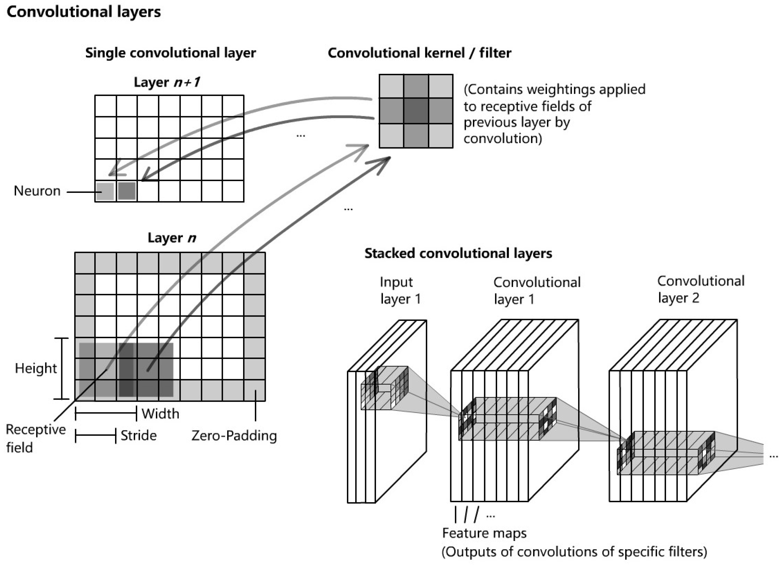
Convolutional Neural Networks are architectures that consist of stacked neural layers of certain functional types. The basis is formed by sequences of convolutional layers and pooling layers. Convolutional layers are sets of convolutional filters that connect the neurons in the current layer to local sections (receptive fields) in the previous layer or input layer (see Figure 5). The filters apply a convolution based on the receptive field size, stride, and weights to the neurons of the previous layers. This process is called feature extraction, as it creates feature maps using activation functions, e.g., ReLU, sigmoid, tanh, etc., that contain information about the most active neurons with regard to that specific filter. A two-dimensional discrete convolution is applied using the following general formula

$$\begin{array}{cc}\hfill S[i,j]& =(I\ast K)[i,j]=\sum _m^{}\sum _n^{}I[i+m,j+n]·K[m,n]\hfill \end{array}$$

(15)

where K is the kernel with the indices m and n, and I is the input or preceding layer with the indices i and j.

The determination of the filter weights is the main task in the learning process. In contrast to fully connected networks (FCNs), this structure reduces the number of weights and, therefore, the computational effort, while preserving a certain degree of generalization. Pooling layers perform a subsampling task to reduce the amount of information and, therefore, the computational load and increase the degree of invariance to slight variations in the data of the previous layer. The most common pooling layer types are the maximum pooling layer and the average pooling layer. The former selects the neuron with the highest value within its specific receptive field, whereas the latter takes the average value of all neurons of the receptive field of the previous layer. Finally, fully connected layers connect the neurons containing the results of the convolutional process to the neurons of the output layer for a classification task through flattening. The degree of generalization can be increased by inserting dropout layers, which reduce the number of neurons.

Seyfioglu, Özbayoglu, and Gürbüz [53] applied a multiclass SVM, an AE, a CNN, and a CAE to classify 12 aided and unaided coarse-grained human activities. Using a 4.0 GHz CW radar system to create spectrograms, domain-specific features, e.g., cadence velocity diagrams (cvds), as well as non-domain features, e.g., cepstral coefficients, LPC, and DCT, were derived. The sample sizes ranged from 50 (sitting) to 149 (wheelchair) for each class. The CAE-based approach achieved the highest accuracy of 94.2%, followed by the CNN (90.1%), AE (84.1%), and multiclass SVM (76.9%).

Singh et al. [48] used a time-distributed CNN enhanced with a Bidirectional LSTM to classify five human full-body activities consisting of boxing, jumping, jacks, jumping, squats, and walking, based on mmWave radar point clouds. The dataset was collected using a commercial off-the-shelf FMCW radar system in the 76–81 GHz frequency range capable of estimating the target direction. The dataset consisted of 12,097 samples for training, 3538 for testing, and 2419 for validation, where each sample consisted of a voxelized representation with dimensions of $60\times 10\times 32\times 32$. Among the other ML-based methods applied (SVM, MLP, Bidirectional LSTM), the accuracy of 90.47% achieved by the CNN was the highest. However, the main drawback of this method is the increased memory requirement for the voxelized representation of the target information, which is not a concern when using micro-Doppler signatures.

Besides Stacked Autoencoders and Recurrent Neural Networks, Jia et al. [41] applied a CNN to a dataset that was collected using an FMCW radar system working at 5.8 GHz. The dataset was used to build features with dimensions of $32\times 32\times 3$ based on the compressed range-time, Doppler-time amplitude and phase, and cadence velocity diagram data [41]. The data were collected from 83 participants performing six activities consisting of walking, sitting down, standing up, picking up an object, drinking, and falling, which were repeated thrice to deliver 1164 samples in total. An accuracy of 92.21% was achieved for the CNN using Bayes optimization, whereas the SAE achieved 91.23%. The SVM-based approach achieved 95.24% accuracy after feature adaptation using SBS, while the accuracy of the CNN was improved to 96.65% by selecting handcrafted features.

Huang et al. [63] used a combination of a CNN and a Recurrent Neural Network (LSTM) model as a feature extractor for point cloud-based data and a CNN to extract features from range-Doppler maps. The outputs from both models were merged and fed into an FCN-based classifier to classify the inputs into six activities consisting of in-place actions, e.g., boxing, jumping, squatting, walking, and high-knee lifting. The results showed a very high accuracy of 97.26%, which is higher than the results of the feature extraction methods used in other approaches.

In [64], a CNN model was developed using two parallel CNN networks, whose outputs were fused into an FCN for classification (DVCNN). This approach along with an enhanced voxelization method led to high accuracies of 98% for fall detection and 97.71% for activity classification.

Chakraborty et al. [65] used an open source pretrained DCNN, i.e., MobileNetV2, VGG19, ResNet-50, InceptionV3, DenseNet-201, and VGG16, to train with their own provided dataset (DIAT- $\mu$RadHAR) consisting of 3780 micro-Doppler images comprising different coarse-grained military-related activities, e.g., boxing, crawling, jogging, jumping with a gun, marching, and grenade throwing. An overall accuracy of 98% proved the suitability of transfer learning for HAR.

3.3. Recurrent Neural Networks

Since the works of Rumelhart, Hinton, and Williams [76], as well as Schmidhuber [77], Recurrent Neural Networks (RNN) and their derivatives, i.e., Long Short-Term Memory Networks, have been widely applied in the fields of natural sciences and economics. In contrast to CNNs, which are characterized as neural networks working in a feedforward manner since their outputs depend strictly on the inputs, RNNs have the ability to memorize their latest states, which makes them suitable for the prediction of temporal or ordinal sequences of arbitrary lengths. They consist of interconnected layers of neurons that use the current inputs and the outputs of the previous time steps to compute the current outputs, with shared weights allocated to the inputs and outputs separately using biases and nonlinear functions. By stacking multiple RNN layers, a hierarchy is implemented, which allows for the prediction of more complex time series.

An exemplary structure of an RNN is presented in Figure 6. On the left side, the network architecture is presented using general notation, whereas on the right side, its temporal unrolled (or unfolded) presentation is illustrated, where each column represents the same model at a different point in time. The current input, $x_t$, is required to update the first hidden state, $h_t^i$, of node, i, where i and t denote the node index and time instance, respectively. This update happens along with the previous state of the same node using the weighting matrices, U and $W^i$, and a nonlinear activation function for the output. Then, the output of the node is passed to the next hidden state, $h_t^{i+1}$, as input via the weighting matrix, $V^i$. Last but not least, the model’s output is obtained using another nonlinear activation function. This leads to a structure of interlinked nodes that are able to memorize temporal patterns, where the number of nodes determines the memorability.

Despite their enormous potential for the prediction of complex time series, RNNs suffer from two main phenomena known as unstable gradients and vanishing gradients, which limit their capabilities. The first phenomenon occurs when a complex task involves many layers, which leads to the accumulation of increasingly growing products that cause exploding gradients, whereas the second refers to the problem where the cells, due to their limited structure, tend to reduce the weights of the earliest inputs and states.

3.4. Long Short-Term Memory (LSTM)

In 1997, Hochreiter and Schmidhuber [78] introduced LSTM cells, which have been investigated and enhanced in the works of Graves, Sak, and Zaremba [79,80,81]. In contrast to RNNs, Long Short-Term Memory networks are efficient in managing longer sequences and are able to reduce the problems that lead to the restricted use of simple RNNs. An LSTM cell contains short-term and long-term capabilities, which enable the memorization and recognition of the most significant inputs using three gate controllers (see Figure 7).

The input gate controls the fraction of the main layer output using the input that is used for the memory. For the Peephole Convolutional LSTM, a variation of the standard Peephole LSTM, to be suitable for processing images, it is calculated using the current input, $x_t$, the previous short-time memory, $h_{t-1}$, and the previous long-time memory, $c_{t-1}$. These are multiplied with the corresponding weighting matrices, $W_{x,i}$, $W_{h,i}$, and $W_{x,i}$, using matrix multiplication or element-wise multiplication (denoted as ∗ and ∘, respectively), and passed to a nonlinear function along with a bias term (see Equation (17)). In contrast to the input gate, the forget gate defines the fraction of the long-term memory that has to be deleted. Similarly, the input and both memory inputs are multiplied with the matrices, $W_{x,f}$, $W_{h,f}$, and $W_{x,f}$, respectively, and added to another bias term, prior to being passed to the same nonlinear activation function (see Equation (16)). This forms the basis for the updates of the memory states, where the current long-time memory (or cell state), $c_t$, is calculated as the sum of the previous long-time memory, $c_{t-1}$, weighted by the forget gate and the new candidate for the cell state, which is the tanh-activated linear combination of the weighted input and the previous short-time memory weighted by the input gate (see Equation (18)). Finally, the output gate determines the part of the long-term memory that is used as the current output, $y_t$, and the short-term memory for the next time step. For this, the current short-time memory of the LSTM cell is calculated by the tanh-activated current long-time memory, $c_t$, weighted by the output gate, which itself is calculated using the current input, the previous short-time state, and the current long-time memory state (see Equations (19) and (20)).

$$\begin{array}{cc}\hfill f_t& =\sigma (x_t\ast W_{x,f}+h_{t-1}\ast W_{h,f}+c_{t-1}\circ W_{c,f}+b_f)\hfill \end{array}$$

(16)

$$\begin{array}{cc}\hfill i_t& =\sigma (x_t\ast W_{x,i}+h_{t-1}\ast W_{h,i}+c_{t-1}\circ W_{c,i}+b_i)\hfill \end{array}$$

(17)

$$\begin{array}{cc}\hfill c_t& =f_t\circ c_{t-1}+i_t\circ \tan \mathrm{h}(x_t\ast W_{x,c}+h_{t-1}\ast W_{h,c}+b_c)\hfill \end{array}$$

(18)

$$\begin{array}{cc}\hfill o_t& =\sigma (x_t\ast W_{x,o}+h_{t-1}\ast W_{h,o}+c_t\circ W_{c,o}+b_o)\hfill \end{array}$$

(19)

$$\begin{array}{cc}\hfill h_t& =o_t\circ \tan \mathrm{h}\left(c_t\right)\hfill \end{array}$$

(20)

Vandermissen et al. [46] used a 77 GHz FMCW radar to collect data from nine subjects performing 12 different coarse- and fine-grained activities, namely events and gestures. Using sequential range-Doppler and micro-Doppler maps, five different neural networks, including an LSTM, a 1D CNN-LSTM, a 2D CNN, a 2D CNN-LSTM, and a 3D CNN, were investigated using 1505 and 2347 samples of events and gestures with regard to performance, modality, optimal sample length, and complexity. It was shown that the 3D CNN resulted in an accuracy of 87.78% for events and 97.03% for gestures.

Cheng et al. [57] derived a method for through-the-wall classification and focused on the problem of unknown temporal allocation of activities during recognition, which can significantly impact accuracy. By employing Stacked LSTMs (SLSTMs) embedded between two fully connected networks (FCNs) and using randomly cropped training data within the Backpropagation Through Random Time (BPTRT) method for the training process, an average accuracy of 97.6% was achieved for the recognition of four different coarse-grained activities (punching three times, squatting and picking up an object, stepping in place, and raising hands into a horizontal position).

In [59], an SFCW radar system was employed to produce spectrograms for multiple frequencies in the collection of data from 11 subjects who performed six different activities with transitions. By comparing the single-frequency LSTM and Bi-LSTM with their multi-frequency counterparts, it was shown that the classification performance was significantly higher, resulting in accuracies of 85.41% and 96.15%.

Due to their ability to memorize even longer temporal sequences, which applies to a wide range of human activities, LSTM networks are, in general, suitable for radar-based HAR, as long as the limitations are considered. RNNs also have limitations, i.e., numerical problems with the determination of gradients and setup constraints due to the sample lengths of input data [46]. Moreover, in comparison with other techniques, LSTM networks require a high memory bandwidth, which can be a major drawback in online applications if hardware with limited resources is used [82].

3.5. Stacked Autoencoders

For a variety of applications, dense or compressed representations of input data using unlabeled data are required to reduce dimensionality by automatically extracting significant features. Autoencoders and modifications of them have proven their suitability across a variety of fields, especially in the image-processing domain. A basic autoencoder (AE) consists of an encoder, which generates a latent representation of the input data in one hidden layer of much lower dimensionality (codings), and a decoder, which reconstructs the inputs based on these codings. By using Stacked Autoencoders (SAEs) that have multiple symmetrically distributed hidden layers (stacking), the capability to handle inputs that require complex codings can be extended (see Figure 8).

Jokanovic et al. [8] used an SAE for feature extraction and a softmax regression classifier for fall detection. Among the positive effects of the proposed preprocessing method, an accuracy of 87% was achieved.

Jia et al. [41] used an SAE, in addition to an SVM and a CNN, to evaluate performance using multidomain features, i.e., range-time (RT), Doppler-time (DT), and cadence velocity diagram (CVD) maps, based on an open dataset [35] and an additional dataset. It was shown that for different feature fusions, the CNN was the most robust method, followed by the SAE and the SVM.

3.6. Convolutional Autoencoders

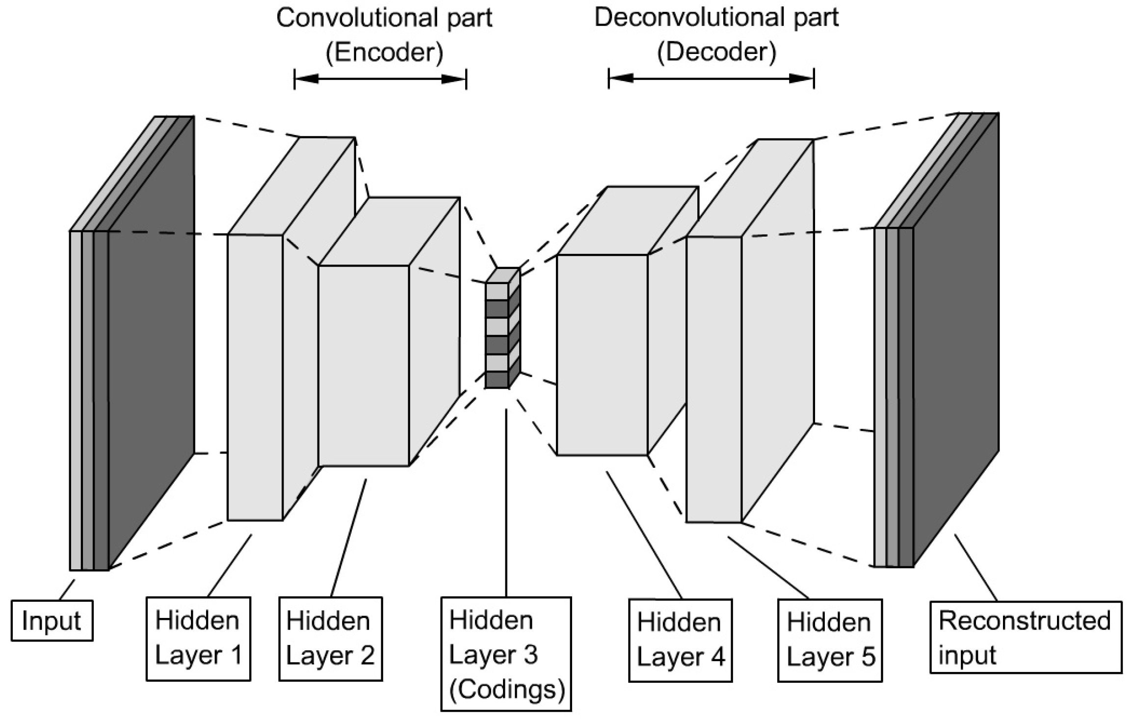
When useful features of images form the basis of an application, Convolutional Autoencoders (CAEs) are better suited than SAEs due to their capability of retaining spatial information. Their high-level structure is equal to that of a simple autoencoder, namely the sequence of an encoder and a decoder, but in this case, both parts contain CNNs (see Figure 9).

Campbell and Ahmad [56] pursued an augmented approach, where a Convolutional Autoencoder was used for a classification task using local feature maps for the convolutional part and the whole signature for the multi-head attention (MHA) part. MHA is an aggregation of single-attention heads, where each head is a function of three parameters: query, key, and value. The dataset was established using a 6 GHz Doppler radar to collect data from five subjects based on coarse-grained activities (falling, bending, sitting, and walking [56]), where each activity was repeated six times. The study was carried out for different training and test split sizes. From the results, it was observed that the attention-based CAE required less data for training compared to the standard CAE with up to three layers, achieving an accuracy of 91.1% for the multi-head attention using a multi-filter approach.

A comprehensive overview of key articles with regard to the radar technology domain, data, classification method, and achieved results is provided in

Table A1. Radar classes and echo signals used for coarse-grained HAR.

Ref.	Year	Radar Type	Center Freq./GHz	Features	Dataset, Samples	Activities	Class. Model	Process.	Max. Accuracy/%
[40]	2010	FMCW	4.3	Time-based RF signatures	Own; 40 per class (5 of 7)	Walk, run, rotate, punch, crawl, standing still, transition (standing/sitting)	SVM	PCA	89.99
[53]	2018	CW	4.0	DT, CV, etc.	Own; 50–149	Walk, jog, limp, walk + cane, walk + walker, walk + crutches, crawl, creep, wheelchair, fall, sit, falling (chair)	CAE	-	94.2
[47]	2018	CW	24.0	DT	Own; 50–149	[RadID]	DCNN	-	94.2
[48]	2019	FMCW	76.0–81.0	Range, velocity, power, angle, time	Own (MMActivity): Training: 12,097; Test: 3538; Validation: 2419;	Box, jump (jacks), jump, squats, walk	SVM (with RBF), MLP, LSTM, CNN + LSTM	PCA (for SVM)	SVM: 63.74; MLP: 80.34; Bi-LSTM: 88.42; CNN + Bi-LSTM: 90.47
[41]	2020	FMCW	5.8	RT, RD, amplitude/phase, CV	Own; 249 per class	Walk, sit down, stand up, pick up object, drink, fall	SVM, SAE, CNN	SBS	SVM: 95.24; SAE: 91.23; CNN: 96.65
[46]	2020	FMCW	77.0	RDT	Own; Events: 1505; Gestures: 2347	Events: enter room, leave room, sit down, stand up, clothe, unclothe; Gestures: drum, shake, swipe l/r, thumb up/down	CNN, CNN + LSTM	n.a.	Event-related: 97.03; Gesture-related: 87.78
[56]	2020	CW	6.0	RD	Own; 900 per class	fall, bend, sit, walk	CAE	n.a.	91.1
[57]	2020	FMCW	1.6–2.2	RT	Own; Training: 704; Test: 160	box, squat and pick up, step in place, raise both hands (into horizontal position)	FCN, SLSTM, FCN	n.a	97.6
[42]	2021	FMCW	<6.0, 76.0–81.0	RT	Own; n.a.	Walking, sitting, falling	SVM, Bagged Trees	SVD	95.7 (sub-6GHz), 89.8 (mmWave)
[59]	2021	SFCW	1.6–2.2	DT	Own; 66 (for each 301 data points)	Step in place, walk (swinging arms), throw, walk, bend, crawl	Uni-LSTM, Bi-LSTM	n.a.	Uni-LSTM: 85.41 (avg.); Bi-LSTM: 96.15 (avg.)
[50]	2021	FMCW	5.8	RT, RD, DT	Own; Training: 1325, Test: 348	Walk, sit down, stand up, pick up object, drink, fall	1D CNN-LSTM, 2D CNN, multidomain approach (MDFradar)	n.a.	1D CNN-LSTM: 71.24 (avg.; RT), 90.88 (DT); 2D CNN: 89.16 (RD); MDFR.: 94.1 (RT, DT, RD)
[63]	2022	FMCW	76.0–81.0	RD	Own; 17 persons; 20 s/activity	Boxing, jumping, squatting, walking, circling, high-knee lifting	CNN, CNN–LSTM	-	97.26
[64]	2022	FMCW	60.0–64.0	3D Point Clouds	Own; 4 persons; 10 min/activity	Walking, Sitting down, lying down from sitting, sitting up from lying down, falling, recuperating from falling	CNN	-	98.0
[65]	2022	FMCW	60.0–64.0	3D Point Clouds	Own; 3870	Boxing, crawling, jogging, jumping with gun, marching, grenade throwing	DCNN	-	98.0
[67]	2023	FMCW	60.0–64.0	3D Point Clouds	Own; 5 persons;	Standing, jumping, sitting, falling, running, walking, bending	MM-HAT (own network)	MHSA	90.5
[68]	2023	FMCW	60.0–64.0	RA, RD, RE	Own; 5 persons; 2000	Boxing, waving, standing, walking, squatting	DyLite-RADHAR (own network)	DSC	98.5
[69]	2023	FMCW	79.0	DT	Own; 10 persons	Walking back and forth, sitting in a chair, standing up, picking up object, drinking, falling	LH-ViT (own network)	-	99.5

, which can be found in Appendix A.

3.7. Transformers

In 2017, Vaswani et al. introduced a new deep learning model, called a Transformer, whose purpose was to enhance encoder–decoder models [66]. Originally derived for sequence-to-sequence transductions, e.g., in Natural Language Processing (NLP), Transformers have also gained importance in other fields, e.g., image processing, due to their ability to process patterns as sequences in parallel in capturing long-term relationships, thereby overcoming the difficulties with CNN- and RNN-based models. They consist of multiple encoder–decoder sets, where the encoder is a series containing a self-attention layer and a feedforward neural network, whereas the decoder has an additional layer, the encoder–decoder attention layer, which helps highlight different positions while generating the output.

Self-attention mechanisms are the basis of Transformers. In the first step, they compute internal vectors (query, key, and value) based on the products of the input vectors and weighting matrices, which are then used to calculate scores after computing the dot products between the query vectors and the key vectors of all other input vectors. The scores can be interpreted as the focus intensity. Using the softmax function after normalization, the attention is calculated as the weighted sum of all value vectors. The weighting matrices are the entities that are tuned during training. Using multiple (multi-head) self-attention mechanisms (MHSA) in parallel, it is possible to build deep neural networks with complex dependencies.

Transformers have also been applied in radar-based human activity. In [67], a Transformer was trained as an end-to-end model and used for the classification of seven coarse-scaled tasks, i.e., standing, jumping, sitting, falling, running, walking, and bending. In comparison with the two other benchmark networks, the accuracy of the Transformer was the highest at 90.45%. With a focus on making Transformers more lightweight, in [68], another novel Transformer was developed and evaluated based on two different datasets of participants performing five activities (boxing, waving, standing, walking, and squatting), achieving accuracies of 99.6% and 97.5%, respectively. Huan et al. introduced another lightweight Transformer [69] that incorporated a feature pyramid structure based on convolution combined with self-attention mechanisms. The average accuracy achieved for the public dataset was 91.7%, whereas for their own dataset, it reached 99.5%.

4. Comparative Study

As the investigation of the performance of recently investigated DL-based approaches is typically based on separate studies utilizing differing datasets, this paper aims to enforce comparability by establishing a common basis using the same dataset across a variety of DL methods. In the first study, all models are trained and evaluated using the same dataset and good practical knowledge. An additional study is conducted to highlight the importance of careful preprocessing, i.e., the adjustment of the color value limits of the feature maps using threshold filtering, where the lower limit is varied using three different offsets of −30, −50, and −70 with regard to the maximum color value, and the influence on classification accuracy is investigated. A second study is conducted where the influence of the compression of the feature maps on the accuracy of the selected models is investigated for three compression ratios.

4.1. Methodology

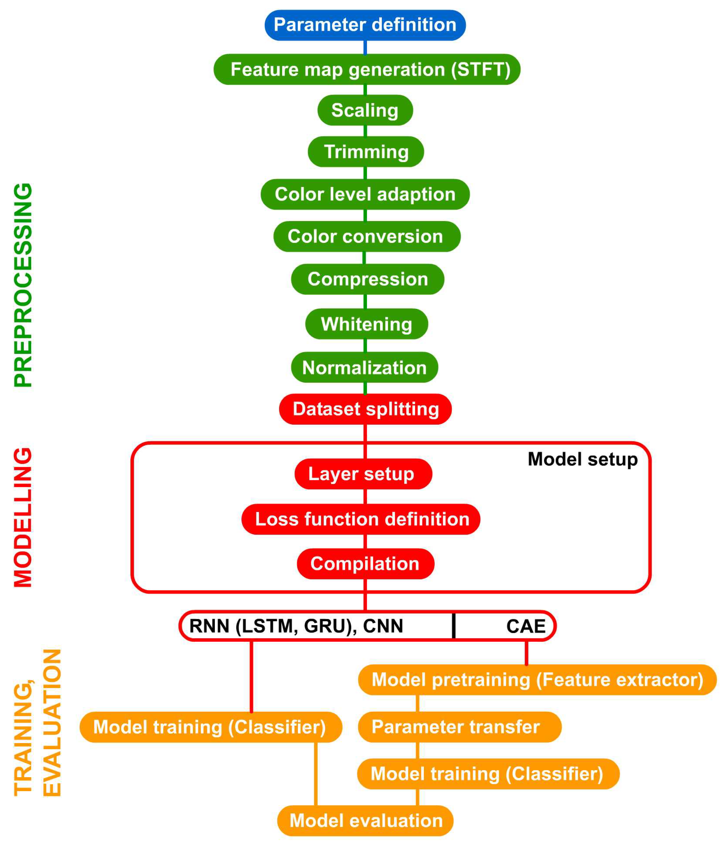
The methodology is expressed in a flowchart that describes the basic procedure (see Figure 10). In the first step of preprocessing, the dataset was used to generate the images containing the feature maps, i.e., Doppler-time maps. After scaling and trimming, the color levels were adapted. In order to reduce dimensionality, the colors were converted to grayscale. Using compression, the image sizes were reduced. Whitening was performed to decorrelate the data without reducing dimensionality. Next, the dataset was split into training, validation, and test datasets. In the model setup, the model for the classifier was defined, and depending on the model architecture, an additional model for pretraining was defined if necessary. The procedure concluded with the evaluation of the model. Since the classes were balanced, performance metrics such as accuracy, recall, and confusion matrix were suitable for the evaluation.

4.2. Dataset

In this study, we used the open dataset Radar Signatures of Human Activities [35], which was recently used by Zhang et al. [83] to produce hybrid maps and train the CNN architectures LeNet-5 and GoogLeNet for classification and benchmarking, respectively, using transfer learning. Jiang et al. [54] used this dataset for RNN-based classification with an LSTM-based classifier, achieving an average testing accuracy of 93.9%. Jia et al. [41] used this dataset for the evaluation of SVM-based classification with varying kernel functions, achieving accuracies between 88% and 91.6%.

The dataset contained a total of 1754 data samples, stored as .dat files containing raw complex-valued radar sensor data of 72 subjects aged from 21 to 88 performing up to six different activities: drinking water (index 0), falling (index 1), picking up an object (index 2), sitting down (index 3), standing up (index 4), and walking (index 5) [35] (see

Table 1. Contents of the open dataset Radar Signatures of Human Activities [35].

No.	Date	Number of Files	Number of Activities	Number of Subjects	Number of Repetitions
1	December 2017	360	6	20	3
2	March 2017	48	6	4	2
3	June 2017	162	6	9	3
4	July 2018	288	6	16	3
5	February 2019	306	6	17	3
6	February 2019	301	5	20	3
7	March 2019	289	5	20	3

). The data were collected using a 5.8 GHz Ancortek FMCW radar, with a chirp duration of 1 ms, a bandwidth of 400 MHz, and a sample time of 1 ms. Each file, which was either about 7.5, 15, or 30 MB in size, contained the sampled intermediate radar data of one particular person performing one activity at a specific repetition.

It must be noted that there was a class imbalance. The activity class falling (index 1) contained a total of 196 sample images, whereas the other classes contained 309 or 310 sample images.

4.3. Development Platform

The comparative study was conducted using an Intel Core i7-1165G7 processor with an Intel Iris Xe graphics card. The embedded graphics card is capable of using 96 execution units at 1300 MHz. In addition, 16 GB of total workspace was available.

The methods were developed using Python-based open source development platforms and APIs: TensorFlow 2.13.0, Keras 2.13.0, and scikit-learn 1.3.1, among other basic toolboxes, e.g., numpy 1.24.3, pandas 2.1.0, and others.

4.4. Data Preprocessing

The data were converted to Doppler-time maps in JPEG format using a Python script, which was developed based on the provided MATLAB file. The function transformed the sampled values of the raw radar signal into a spectrogram (see Figure 11). In the first step, the data were used to calculate the range profile over time using an FFT. Then, a fourth-order Butterworth filter was applied, and the spectrogram was calculated by applying a second Fourier transform to overlapping time-specific filtering windows, i.e., the Hann window. Subsequently, the spectrograms were imported into the Python-based application and transformed into images of $224\times 224\times 3$ px in size after scaling. Trimming the edges and adapting the color levels was important to remove weak interfering artifacts and highlight characteristic patterns caused by frequency leakage or non-optimized windowing. In the next step, they were converted to grayscale images to reduce dimensionality since in this case, the color channels did not contain any additional information. A compression using truncated SVD was applied to reduce the data size while retaining the main information.

Using the ZCA method, the images were whitened. Dimensionality reduction was discarded to avoid significant loss of information. As the color values ranged from 0 to 255, normalization was then applied, which scaled the values from 0 to 1 in order to improve performance.

4.5. Model Setup

For the assessment, a variety of models from three deep learning classes were implemented: Convolutional Neural Networks (CNNs), Recurrent Neural Networks (RNNs), and Convolutional Autoencoders (CAEs) with fully connected networks.

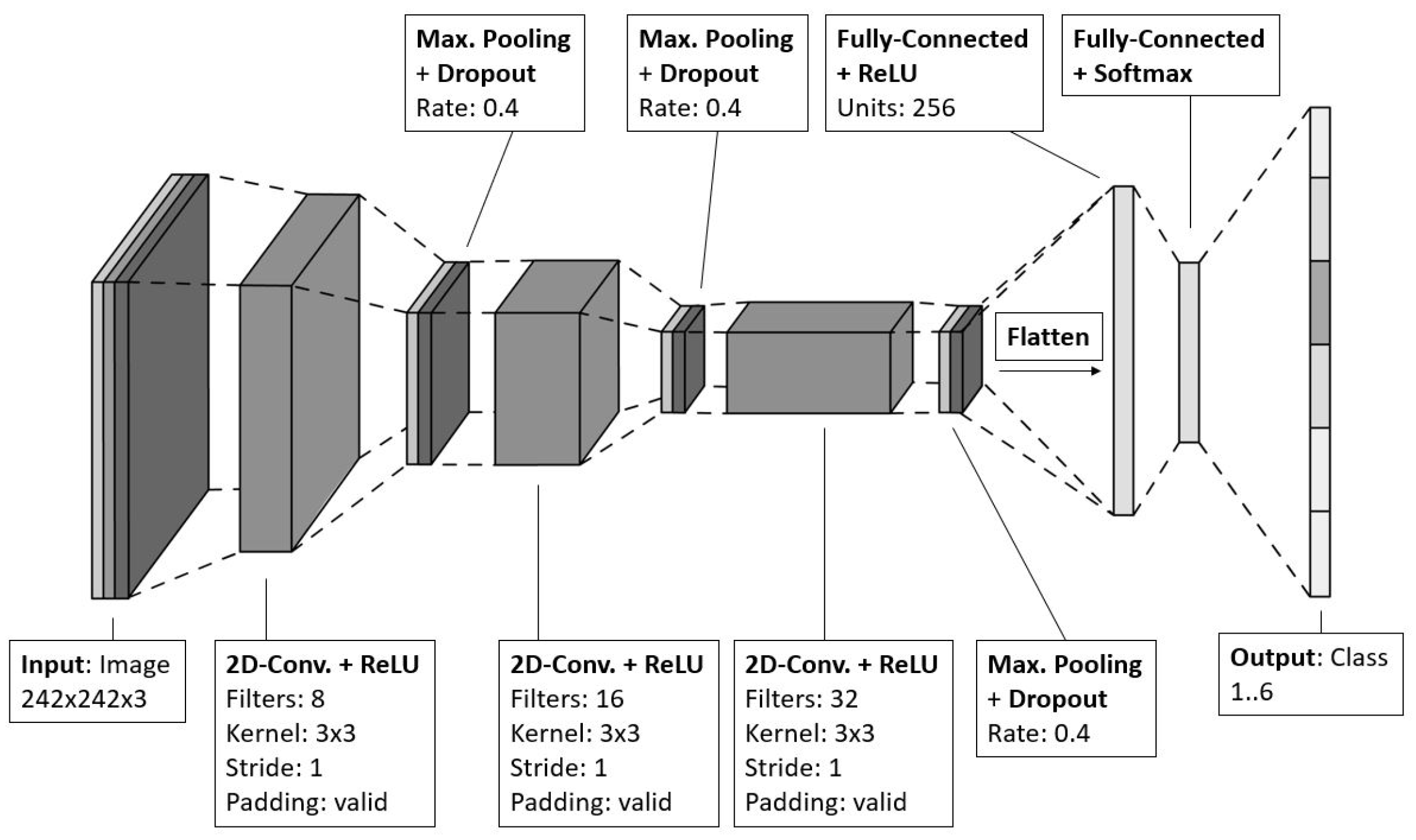
The CNN model consisted of three instances of 2D convolutional layers, where each was followed by a maximum pooling layer and a dropout layer. Next, the network concluded with a flattening layer for implementing vectorization and connecting to two fully connected layers (see Figure 12). The architecture was implemented based on the Keras sequential API using the Input, Conv2D, MaxPooling, Dropout, Flatten, and Dense layer functions; the SGD and Adam optimizers; and the Categorical Cross-Entropy loss function from the keras.layers, keras.optimizers, and keras.losses packages, respectively.

The increasing number of filters in each convolutional layer helped build hierarchical features and prevent overfitting. The first layers captured low-level information, whereas the last ones reached higher levels of abstraction with higher complexity and became smaller to enforce generalization. The 3-by-3 kernel, with a stride of 1 and without padding, was required to halve the dimensions of the feature maps until the smallest size was reached, producing good results—28 × 28. The values for the penalty function of the regularizers for the kernel, bias, and activity were set to be $1.0\times {10}^{-2}$, $1.0\times {10}^{-4}$, and $1.0\times {10}^{-5}$, which were good empirical values to start with. A Rectified Linear Unit (ReLU) activation function was selected for faster learning. The comparably average dropout rate of 0.4 was well-suited for this network since the aforementioned regularizers had to be taken into account. The first downstream FCN, which consisted of 212 nodes and connected the last maximum pooling layer with the output FCN, was used for the classifier. It was required to transform the spatial features of the feature maps into complex relationships. The output FCN had six nodes, each representing one class and using a softmax activation function to determine the probability of class assignment for the input image.

The RNN models were constructed using simple RNNs, LSTMs, Bidirectional LSTMs, and Gated Recurrent Units (GRUs), which were also implemented based on the Keras sequential model using the SimpleRNN, LSTM, GRU, Bidirectional, and Dense layer functions from the keras.layers package.

The number of nodes in the first part, which was the recurrent network, was uniformly set to 128, which led to good results and prevented overfitting. For activation, the hyperbolic tangent function (tanh) was selected, as it is associated with bigger gradients and, in comparison with the sigmoid function, faster training. Each network was followed by a fully connected layer to establish the complex nonlinear relationships required to connect the time-specific memory to the respective classes. Using a softmax function for activation, the probabilities were outputted for each class.

The autoencoder-based model was implemented based on the architecture of the CAE (see Figure 13). In contrast to the aforementioned implementation, it used the Keras functional API, as it is more flexible and allows for branching and varying the numbers of inputs and outputs. The branching option was required to independently define the encoder and decoder parts since two consecutive training sessions were required. The first training (pretraining) was performed on the complete autoencoder model consisting of the encoder and decoder parts to train the feature-extracting capabilities. Then, the trained weightings and biases were transferred to a separate model consisting of the encoder part and an FCN, which implemented the classifier, to output the class probabilities.

4.6. Training

For training, 70% of the total training dataset was used as the training subset, employing cross-validation with batches of 32 samples for up to 300 epochs. For validation, 20% of the dataset was used; hence, 10% of the dataset was used as the test subset. The model-specific numbers of parameters are listed in

Table 2. Number of parameters for each of the investigated methods.

Method	Trainable	Non-Trainable	Total
CNN	4,853,174	0	4,853,174
LSTM	494,086	0	494,086
Bi-LSTM	988,166	0	988,166
GRU	371,718	0	371,718
CAE	25,691,910	94,144	25,786,054

.

Depending on the network, either the Stochastic Gradient Descent (SGD) algorithm or Adam (adaptive moment estimation) optimizer was used, with individual and optimized learning rates for each network that varied between ${10}^{-3}$ and ${10}^{-4}$.

5. Results

For the performance evaluation, the standard ML metrics (accuracy, recall, precision, and F1 score) were selected. Due to the class imbalance, i.e., unequal sample size between the activity of falling (index 1) and the other activities, the measures of accuracy, recall, and precision were expected to have slight errors, which is of little relevance, since the relations were the main interest. The F1 score has the robustness to overcome this issue since it compensates for the tendency of the recall to underestimate and the precision to overestimate using the harmonic mean calculated from both. Two additional metrics (the macro-averaged Matthew Correlation Coefficient (MCC) and Cohen Kappa) are also robust against class imbalances and, along with the F1 score, form the basis for the assessment. The MCC, which has its origin in binary classification, can be used to evaluate classifiers’ performance in a multiclass classification task when a one-vs.-all strategy is pursued. In this case, a classifier’s performance is computed using the average of the performance of every classifier, where each one can only classify a sample as belonging to the class assigned or, conversely, as belonging to any of the remaining classes. The Cohen Kappa measures the degree of agreement between different classifiers, where in this case, the probabilities of agreement between the classifiers in a one-vs-all strategy, along with the probabilities for a random-driven agreement, are considered.

The metrics of the results of the classification studies are listed in

Table 3. Performance results and execution times for validation for the investigated methods.

Method	Accuracy%	Precision%	Recall%	F1%	MCC%	Cohen Kappa%	Total Execution Time/s
CNN	88.0	89.7	88.0	87.9	86.0	91.0	3251
LSTM	82.3	85.6	82.9	83.0	80.1	85.5	2966
Bi-LSTM	86.3	88.7	86.3	86.8	83.7	90.2	10,780
GRU	82.3	82.6	82.3	82.0	78.8	86.0	2569
CAE	81.7	84.2	81.7	82.5	78.1	78.1	7349

. The learning curves, consisting of the loss and accuracy functions, as well as the resulting confusion matrices, are displayed in Figure 14, Figure 15, Figure 16, Figure 17 and Figure 18.

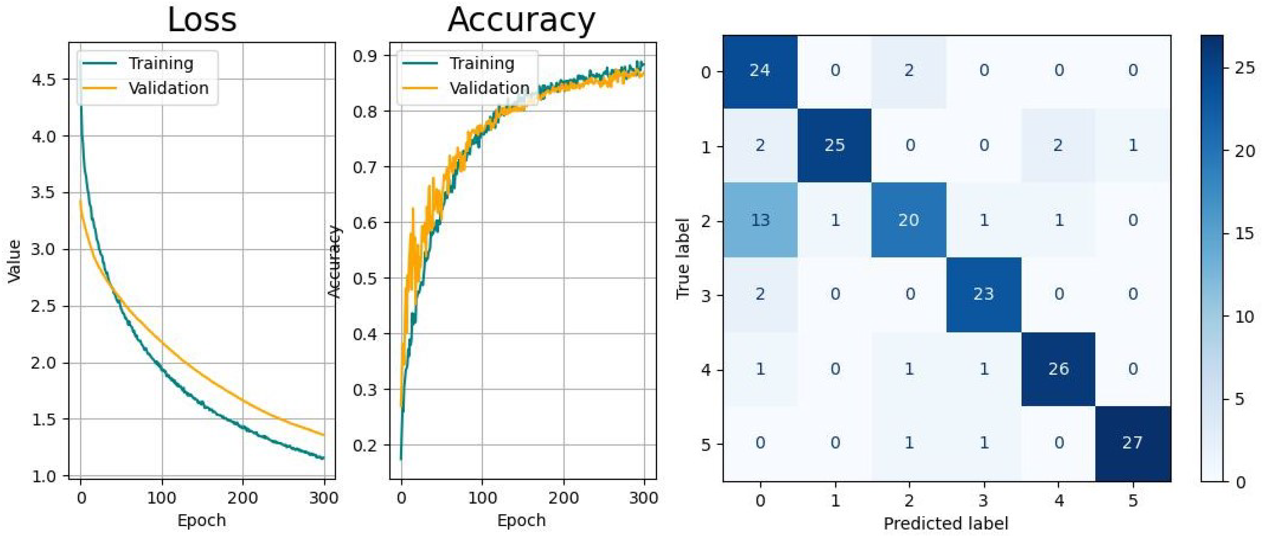
The learning curves of the CNN (Figure 14) show a moderate learning pace with decreasing variance and the likelihood of sudden spikes that tend to appear when using the Adam optimizer. The decreasing gap between the training and validation curves indicates the absence of overfitting. From the confusion matrix, it is evident that there is a higher probability of the network confusing the activity of picking up objects with drinking, while the other tasks remain unaffected.

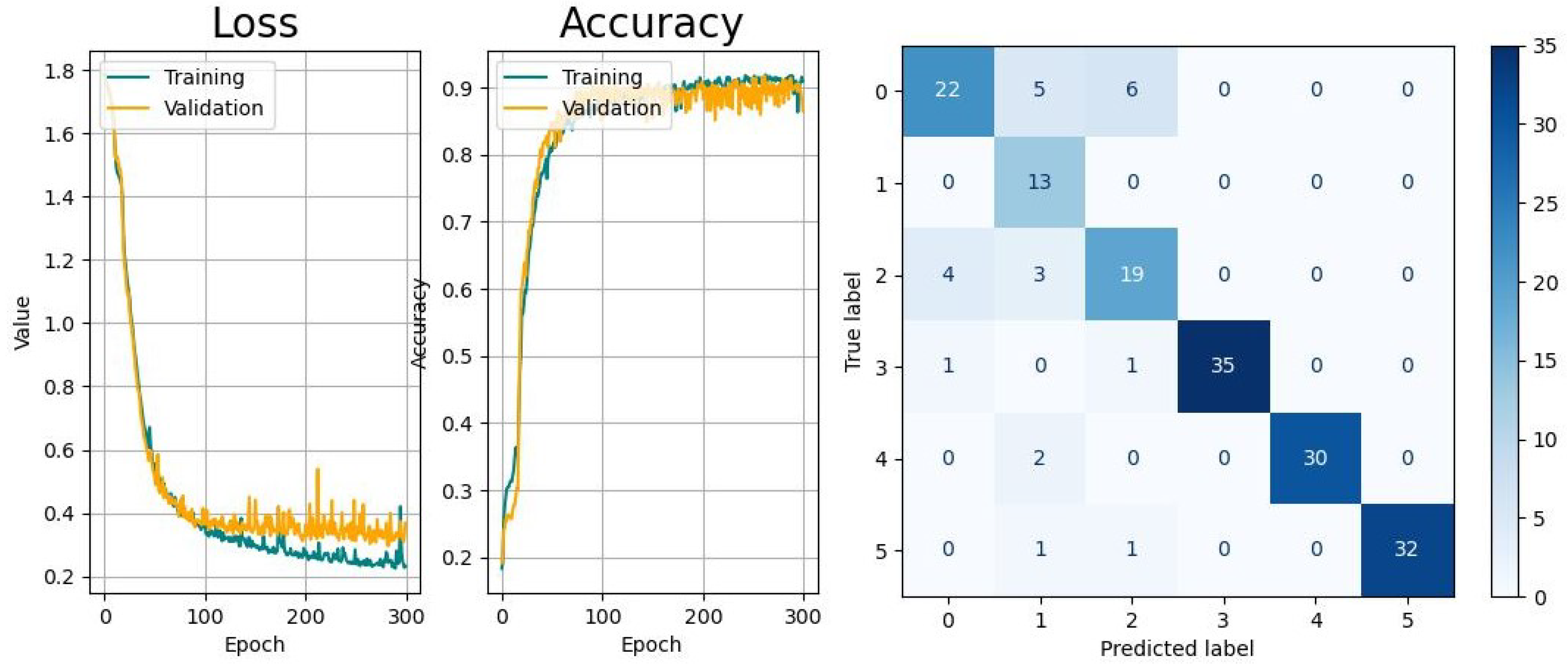
The learning curves of the RNN-based networks show varying performances. The LSTM network has similar learning curves to the CNN with regard to the learning pace and generalization, and the confusion matrix shows the same issue as the CNN. The learning curves of the Bi-LSTM show significantly faster convergence but suffer from higher variance, although the confusion is significantly smaller compared to the aforementioned models. The GRU network shows a higher tendency toward overfitting, with comparably small variances in accuracy progress. Last but not least, the CAE network shows the biggest tendency to overfit and, besides the confusion between tasks 0 and 2, has an increased risk of confusing task 0 (drinking) with task 4 (standing up).

The influence of the color levels of the feature maps on performance is shown in Figure 19. This variational study was carried out for all models, where the lower limit of the color scale was varied using offsets of −30 (least details), −50, and −70 (most details) with regard to the maximum color value. Here, the CAE and CNN show the best performance and higher robustness to color level variations, whereas the RNN-based methods are more strongly affected, with the GRU showing the strongest effects. The results indicate that the color levels have a significant impact on classification accuracy. Considering the stochastic effects of training, the optimum threshold in this study probably lies between −50 and −70.

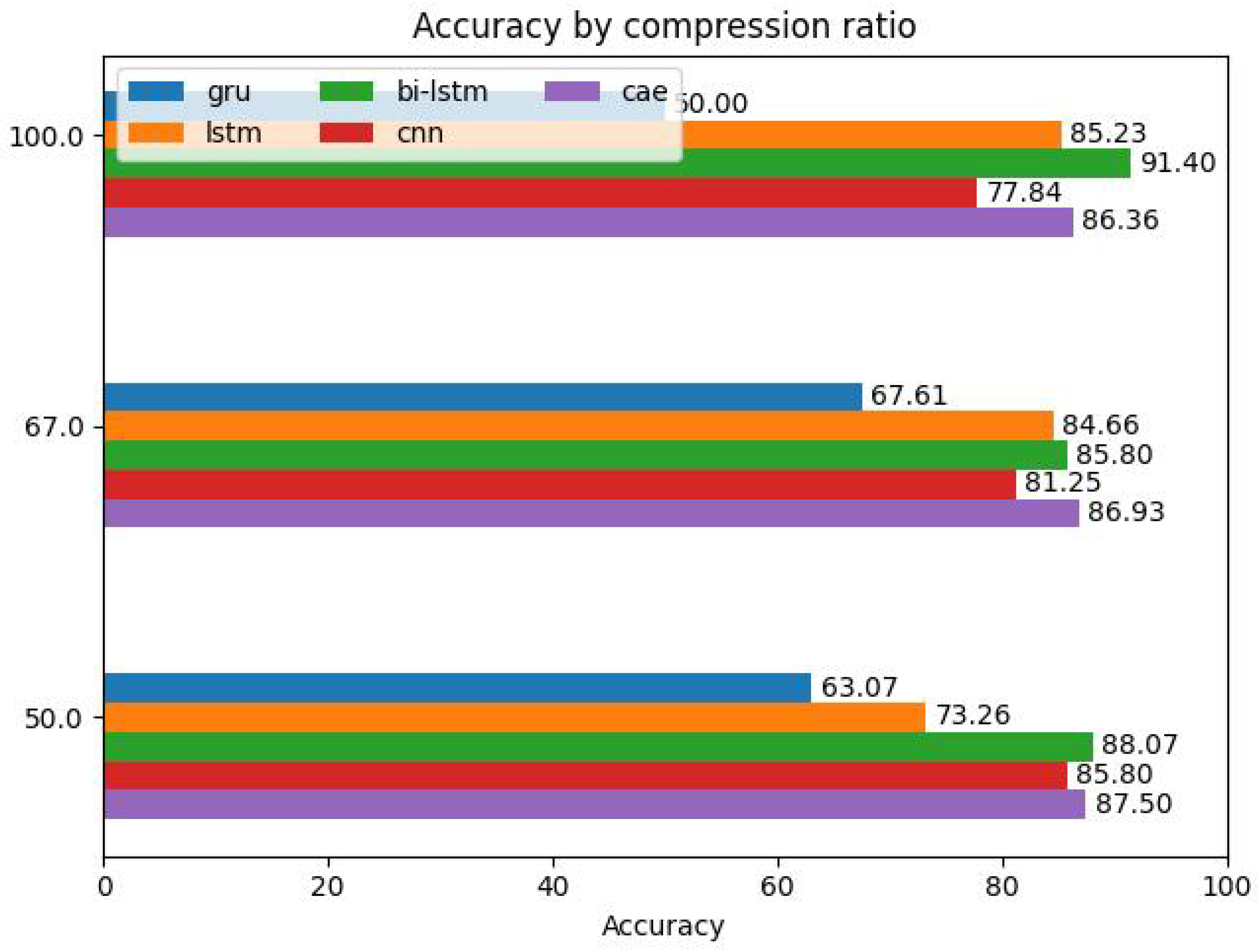
The influence of the compression ratios of the feature maps on performance is shown in Figure 20. Using three different compression ratios, i.e., 100%, 67%, and 50%, a study was carried out for all models. According to the results, the performance of all models, except for the GRU, shows high robustness to information loss caused by compression, with the CAE achieving the best results, followed by the CNN and Bi-LSTM. In practice, this means that even with a halved data size, the models are able to achieve similar performance. It should be noted that the model-specific performance deviations in the investigated cases were caused by the stochastic nature of the learning algorithm and the dataset batching process.

From the results, we can confirm that CNN-based classification achieved better performance in comparison to the investigated RNN-based methods. The reason for this is that the derived feature maps of CNNs have the ability to extract locally distributed spatial features in a hierarchical manner and, therefore, can recognize typical patterns, whereas RNN-based methods memorize temporal sequences of single features. This ability also applies to CAEs, but the tendency for overfitting is much higher, so tuning, e.g., through better regularization, is necessary. Regarding the underlying type of input, namely images, RNN-based networks are suboptimal due to the lack of scalability and the absence of the ability to memorize spatial properties.

Further, it can be revealed that the classification of coarse-grained activities led to better results. Higher magnitudes of the reflected radar signal, which were assigned to large-scale movements, led to distinct characteristic properties in the micro-Doppler maps, which improved performance.

6. Discussion

According to the metrics of the validation, all models yielded acceptable results for the same dataset, indicating their overall suitability for this application with different levels of performance. In addition, the learning curves of all models were convergent but indicated different levels of smoothness and generalization. Further, it can be confirmed that the misclassifications for all models were the highest for the activities of drinking (index 0) and picking up objects (index 2).

The results show that CNNs are more suitable structures for the given task compared to the RNN variants, i.e., LSTM, Bi-LSTM, and GRU, due to their ability to memorize spatial features, while the learning curves tended to show sudden jumps during the first third of the training, followed by smooth and gradual improvements. It is remarkable that the training and validation curves of both the CNN and LSTM networks exhibited significant differences, while their metrics were similar.

Despite the observation that every consecutive run of the training led to slightly different curves, especially the continuity during the first 100 epochs, the variation in validation accuracy was the highest for the Bi-LSTM network, while the training and validation curves had very steep slopes during the same period. Only the GRU network was able to achieve better continuity, but it showed a higher tendency for overfitting during the final epochs.

Further, the overall performance was lower compared to the results mentioned in the aforementioned literature, which suggests that more intensive hyperparameter tuning for the network setup or image generation could improve the results. Another option would be applying a more sophisticated preprocessing technique when generating the samples, specifically, enhancing task-specific pattern details while adapting the conditions to the model’s structure and increasing the overall training time.

7. Conclusions

In this paper, several DL-based approaches that have been the focus of radar-based human activity recognition were reviewed and evaluated. This was performed using a common dataset to evaluate performance across different metrics while accounting for computational cost, which is represented by the overall execution time. The aim was to establish a baseline comparison using the same dataset that assists in selecting the most appropriate method considering the performance and computational cost.

Besides the proposed measures, i.e., model improvement and sample refinement, the application of further DL methods, e.g., autoencoder variants (SAE, CVAE); Generative Adversarial Networks (GAN) and their variants, e.g., Deep Convolutional Generative Adversarial Networks (DCGAN); or combinations of different methods, would broaden the knowledge base. By evaluating additional aspects like sample space or computational space requirements during training, the parametricity of the models, or aspects related to execution, such as the ability to distribute and parallelize operations among multiple computers, new criteria for the selection of the most appropriate DL method could be introduced.