Ore Rock Fragmentation Calculation Based on Multi-Modal Fusion of Point Clouds and Images

Abstract

The accurate calculation of ore rock fragmentation is important for achieving the autonomous mining operation of mine excavators. However, a single mode cannot accurately calculate the ore rock fragmentation due to the low resolution of the point cloud mode and the lack of spatial position information of the image mode. To solve this problem, we propose an ore rock fragmentation calculation method (ORFCM) based on the multi-modal fusion of point clouds and images. The ORFCM makes full use of the advantages of multi-modal data, including the fine-grained object segmentation of images and spatial location information of point clouds. To solve the problem of image under-segmentation, we propose a multiscale adaptive edge-detection method based on an innovative standard deviation map to enhance the weak edges. Furthermore, an improved marked watershed segmentation algorithm is proposed to solve the problem of low segmentation accuracy caused by excessive noise of the gradient map and weak edges submerged. Experiments demonstrate that ORFCM can accurately calculate ore rock fragmentation in the local excavation area without relying on external markers for pixel calibration. The average error of the equivalent diameter of ore rock blocks is 0.66 cm, the average error of the elliptical long diameter is 1.42 cm, and the average error of the elliptical short diameter is 1.06 cm, which can effectively meet practical engineering needs.

1. Introduction

Ore rocks are the main focus of excavation by intelligent electric mining shovels and are formed after blasting in the mine. However, the size of the resulting ore rock fragments can vary due to factors such as the burst point distribution and ore properties, as shown in Figure 1. The collision of the shovel bucket with large chunks of ore can cause equipment damage, such as shovel tip fractures, and even lead to hazardous incidents, like landslides. To address this problem, it is necessary to calculate ore rock fragmentation within the localized excavation area. Ore rock fragmentation calculation refers to the division of each rock block in the local excavation area and then calculating the size of the ore rocks based on the spatial position information of points or pixels. It is essential for enabling autonomous excavation and ensuring the safe operation of intelligent electric shovels.

The existing research methods for determining the size of ore blocks primarily rely on image segmentation or image edge detection algorithms. While leveraging fine-grained information, such as color or texture, in image modalities has proven beneficial for segmenting distinct ore blocks, these images inherently lack spatial position information, posing a challenge in accurately computing ore block sizes directly from image data. To address this challenge, some researchers have employed the placement of specific markers to calibrate image pixels [1]. However, these approaches are inconvenient and impractical for mining shovel operations, limiting their applicability in real-world scenarios. In recent years, the widespread adoption of LiDAR technology has prompted researchers to use three-dimensional point cloud data for calculating the sizes of ore blocks [2]. In the point cloud modality, the spatial and geometric position information of the ore rock point cloud can be directly utilized for size calculations. However, 3D point clouds obtained from vehicle-mounted 3D LiDAR systems typically have lower resolutions compared with images. Moreover, point cloud data often lack fine-grained information, such as color and texture. This limitation can impact the effectiveness of mine rock segmentation, thereby reducing the accuracy of rock block size calculations.

To address the aforementioned challenges, this research paper proposes a novel approach that integrates point cloud and image multimodalities for calculating the size of rock fragments. This method capitalizes on the high resolution and comprehensive color–texture information available in the image modality to generate segmented images of ore and rock blocks. Firstly, the mapping relationship between the image and point cloud mode is established based on the joint calibration of the camera and LiDAR. Then, the pixels in the segmented map are dimensionally calibrated using the spatial position information of the point cloud modality. As a result, accurate computations of rock block sizes are achieved. This approach maximizes the fusion potential of point cloud and image multimodalities and effectively utilizes the spatial position information from the point cloud modality, as well as the high-resolution capabilities and texture information from the image modality. By synergistically integrating these modal data, the method overcomes the limitations of relying on a single modality for calculating rock fragment sizes. This integration significantly enhances the accuracy and practicality of the algorithm, leading to improved overall computation accuracy.

2. Related Works

2.1. Computation Methods Based on the Image Modality

Currently, researchers mostly use traditional image processing methods to calculate ore rock fragment sizes. Amankwah et al. [3] proposed a method for rock image segmentation using mean shift and watershed transformation to estimate block dimensions. Zhang et al. [4] introduced a threshold segmentation technique based on Fisher’s discriminant bidirectional window, which exhibited good edge preservation and noise resistance in ore rock images. Wang et al. [5] utilized an improved watershed algorithm for rock segmentation and computed the distribution of rock block sizes by analyzing the projected diameters of mineral particles. Guo et al. [6] proposed an adaptive watershed segmentation algorithm based on the shape of rock blocks, which solved the segmentation errors caused by adhesion and edge blur in images of blasting rock piles. Ding et al. [7] simplified the process by computing the gradient map of rock images using the Sobel operator and extracting rock block contours through image binarization. By analyzing the size distribution of rock blocks, they established a correlation between blasting parameters and the degree of block fragmentation. Wang et al. [8] utilized the Canny edge detection operator and moment-preserving method to extract the edges of rock block images, achieving precise block segmentation and size calculation. In order to address the weak edge preservation problem in rock images caused by the Otsu thresholding method [9], Zhang et al. [10] introduced an upgraded strategy. They applied the dual-neighborhood technique to select the minimum threshold for image binarization, thereby enhancing the preservation capability of weak edges in rock blocks.

In recent years, there has been an increasing use of neural network-based image processing methods by researchers to address the calculation of rock fragment sizes. Hadi et al. [11] utilized Fourier transform, Gabor, wavelet, and their combinations to extract features from rock images. These features were then fed as inputs to a neural network for computing the size distribution of rock fragments. Xie et al. [12] presented four models that employed gradient enhancement, support vector machine, Gaussian process, and artificial neural network methods to calculate the size distribution of rock fragments. Their main objective was to optimize blasting parameters and enhance the efficiency of open-pit mining operations. Yuan et al. [13] introduced a deep learning-based method for rock image segmentation, utilizing annotated datasets to train an overall nested boundary detection model for segmenting rock blocks. Ko et al. [14] applied image processing techniques to acquire the surface of rock blocks and built a neural network model to analyze the distribution of block sizes. Shubham et al. [15] constructed a convolutional neural network based on Mask R-CNN [16] for predicting the size of rock fragments. Xiao et al. [17] combined the residual structure of convolutional neural networks with the DUNet model [18] to propose a rock image segmentation model called RDU-Net. This model can dynamically adjust the receptive field based on the size and shape of different rock fragments. These features enable the accurate capture of the edges of rocks of varying sizes and shapes, leading to effective segmentation of rock images.

2.2. Computation Methods Based on the Point Cloud Modality

With the increasing adoption and extensive use of 3D laser scanning technology in the field of smart mining, researchers have started exploring the calculation of rock fragmentation using 3D point cloud modalities. Matthew et al. [19] proposed a method for calculating rock fragmentation based on the laser scanning of rock point clouds. The process involved rasterizing the 3D point cloud data of rocks and employing a combination of the watershed algorithm and morphological operators to segment the rock fragments. The positional spatial information of the edge points of rocks was then utilized to determine the degree of rock fragmentation. To address the challenges associated with perspective distortion and limited utilization of spatial information in image-based methods for calculating rock fragmentation, Onederra et al. [20] employed high-resolution 3D laser scanning to capture rock point cloud data. They utilized a combination of morphological edge detection and watershed segmentation algorithms to effectively segment the rock fragments from the point cloud. In another study conducted by Campbell et al. [21], high-resolution 3D laser scanning was utilized to obtain rock point cloud data. The point cloud underwent preprocessing using filtering and orthogonal projection techniques. Subsequently, the segmentation of rock fragments from the point cloud was achieved through morphological edge detection and the watershed algorithm. Finally, the segmented point cloud underwent inverse projection to compute the degree of rock fragmentation. To overcome the limitations and inaccuracies of image analysis methods, Engin et al. [22] utilized laser scanning technology to directly measure the size distribution of rock fragments.

2.3. Analysis

The current methods for computing rock fragmentation primarily rely on image modalities. However, accurately estimating rock fragmentation becomes challenging due to the limited availability of spatial and geometric information in rock images, which mainly provide color and texture information. To overcome this challenge, researchers have explored alternative approaches, such as using specific markers for image pixel calibration. However, these marker-based techniques are cumbersome and impractical in real-world applications of intelligent mining. In recent years, the increasing use of laser scanning technology has opened up new possibilities for analyzing rock fragmentation by leveraging 3D point cloud modalities. By utilizing the inherent spatial and geometric information present in rock point clouds, this innovative approach enables the direct computation of rock fragmentation. However, it is important to note that point clouds generally have lower resolution compared with images and lack fine-grained data, which can potentially impact the accuracy of edge detection and rock segmentation.

3. Ore Rock Fragmentation Calculation Method

We propose an ore rock fragmentation calculation method (ORFCM) by integrating the point cloud and image modalities. The ORFCM involves several steps, including image preprocessing, the construction of the Standard Deviation Map of the Local Gradient Differences (SDM) [23], multiscale adaptive edge detection based on SDM, the establishment of the edge-enhanced SDM, rock image segmentation using the watershed algorithm, and rock fragmentation calculation based on point cloud and image calibration mapping.

3.1. Image Preprocessing

Image preprocessing is a vital prerequisite and foundational step for subsequent algorithms, encompassing key procedures, such as grayscale conversion and median filtering.

Considering the minimal color variations in rock images, the RGB color image undergoes conversion to a single-channel grayscale image, which can reduce the algorithm’s complexity and enhance computational efficiency. The calculation is performed as follows:

$$I_g\left(i,j\right)=R(i,j)\times 0.299+G(i,j)\times 0.587+B(i,j)\times 0.114$$

(1)

where $I_g\left(i,j\right)$ is the grayscale value of the grayscale image $I_g$ at the $\left(i,j\right)$ pixel, and $R(i,j)$, $G(i,j)$, and $B(i,j)$ are the values of the R, G, and B channels of the color image at the $\left(i,j\right)$ pixel, respectively.

Median filtering is utilized to replace the gray value of the central point with the median gray value of all pixels within the local neighborhood. This technique effectively reduces surface texture variations in ore rock and eliminates isolated noise points. The computation can be expressed as follows:

$$I_0\left(i,j\right)=median\{I_g(i-a,j-b)\},(a,b)\in S,$$

(2)

where $I_0\left(i,j\right)$ represents the grayscale value of the pixel after median filtering and S denotes the filtering template window.

3.2. SDM Calculation

First, the gradient map is computed, and subsequently, an image SDM is constructed by leveraging the statistical properties of local gradient differences. This process effectively enhances the visibility of edge pixels while suppressing noise, leading to a more distinct delineation of edges.

3.2.1. Gradient Map Calculation

This study utilizes the Sobel operator to compute the gradient map. The convolution kernels used in this operator along the x and y directions are constructed as follows:

$$S_x=\left[\begin{array}{ccc}-1& 0& 1\\ -2& 0& 2\\ -1& 0& 1\end{array}\right], S_y=\left[\begin{array}{ccc}1& 2& 1\\ 0& 0& 0\\ -1& -2& -1\end{array}\right],$$

(3)

The gradient maps ${\mathrm{G}}_x$ and ${\mathrm{G}}_y$ are computed as follows:

$${\mathrm{G}}_x=S_x\ast I_0,$$

(4)

$${\mathrm{G}}_y=S_y\ast I_0,$$

(5)

where $\ast$ represents the convolution operation. The gradient magnitude $G\left(i,j\right)$ is computed as follows:

$$G\left(i,j\right)=\sqrt{G_x{\left(i,j\right)}^2+G_y{\left(i,j\right)}^2}$$

(6)

The gradient direction $\theta \left(i,j\right)$ is computed as:

$$\theta \left(i,j\right)=\arctan \left(G_y\left(i,j\right)/G_x\left(i,j\right)\right)$$

(7)

3.2.2. SDM Calculation

The computation of the gradient map effectively suppresses backgrounds with subtle grayscale variations. However, there exists noise in the ore rock images. It struggles to accurately differentiate between edges and noise characterized by pronounced grayscale variations. To address this issue, this research employs the statistical characteristics of local gradient variations to compute the SDM. This approach enables reliable discrimination between edges and noise, enhancing the effectiveness of edge detection.

On the gradient map, the gradient difference $d_{ij}\left(m,n\right)$ between a pixel $G\left(i,j\right)$ and any other pixel in its local neighborhood $N\left(i,j\right)=\{G(i+m,j+n)|-k\le m,n\le k\}$ is determined as follows:

$$d_{ij}\left(m,n\right)=\left|G\left(i+m,j+n\right)-G\left(i,j\right)\right|,$$

(8)

The mean value $M\left(i,j\right)$ is calculated as:

$$M\left(i,j\right)={\displaystyle \sum _{m=-k}^k{\displaystyle \sum _{n=-k}^k{d}_{ij}\left(m,n\right)/\left({\left(2k+1\right)}^2-1\right)}},$$

(9)

The standard deviation S(i,j) is calculated as follows:

$$S\left(i,j\right)=\sqrt{\frac{{\displaystyle \sum _{m=-k}^k{\displaystyle \sum _{n=-k}^k{\left(d_{ij}\left(m,n\right)-M\left(i,j\right)\right)}^2}}}{{\left(2k+1\right)}^2-1}},$$

(10)

Figure 2 presents a comparison of the gradient map and SDM. From Figure 2a, it can be seen that the gradient map successfully distinguishes the background from the foreground. However, it struggles to effectively differentiate between edges and noise within the foreground, leading to a reduction in the accuracy of rock fragmentation segmentation. In contrast, Figure 2b demonstrates that the SDM significantly suppresses noise, minimizing its interference with the rock edges. This establishes a strong foundation for subsequent edge detection and rock block segmentation.

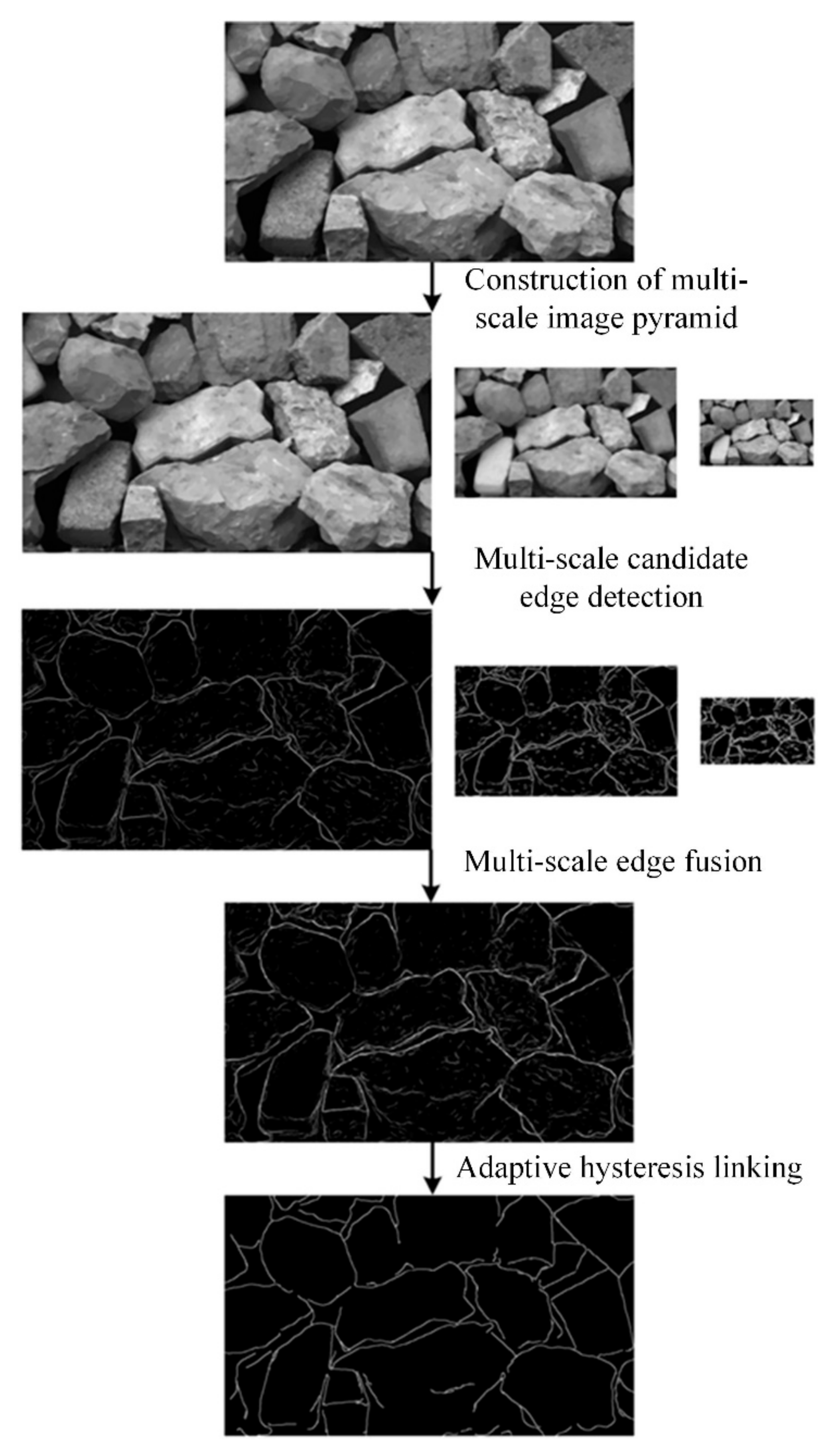
3.3. Multiscale Adaptive Edge Detection Based on SDM

The precise extraction of rock edges can be achieved through a multiscale adaptive image edge detection algorithm based on SDM [23], which is proposed in our previous research. The main steps of this algorithm are depicted in Figure 3.

The construction of a multiscale image pyramid enhances the utilization of multiscale information, thereby improving the robustness of edge detection against variations in image scale. At each scale, candidate edge detection is performed using the gradient map and SDM. This approach effectively discriminates between weak edges and noise, leading to improved accuracy in edge detection. The algorithm conducts multiscale edge fusion based on a voting mechanism. This method utilizes multiscale edge features to maximize noise resistance and ensure the continuity of the fused edge images. An adaptive hysteresis connection is applied to the fused edge map using the 2D Otsu method and the 2D maximum entropy method. This process ultimately generates the edge maps E of the rock images.

3.4. Edge-Ehanced SDM Calculation

In mineral rock images, when there is a small grayscale difference between catchment basins and watershed regions, the watershed algorithm is prone to flooding, resulting in under-segmentation issues. This, in turn, reduces the accuracy of rock mass calculation. To address this issue, an edge-enhancement technique is applied to the SDM based on the mineral rock edge map E. This enhances the distinction between the watershed and catchment basins, thus preventing the submersion of critical edges if, and only if, the pixels $E(i,j)$ on the edge map E and the corresponding pixels $S(i,j)$ on the standard deviation map S satisfy the following conditions:

$$\left\{\begin{array}{c}E\left(i,j\right)=255\\ S\left(i,j\right)\ge s_m\end{array}\right.,$$

(11)

where $s_m$ is the median value of all pixels on the standard deviation map S; the pixel value $S\left(i,j\right)$ on the standard deviation map is set as:

$$S\left(i,j\right)=255.$$

(12)

If the condition is not satisfied, the pixel value on the standard deviation map S remains unchanged.

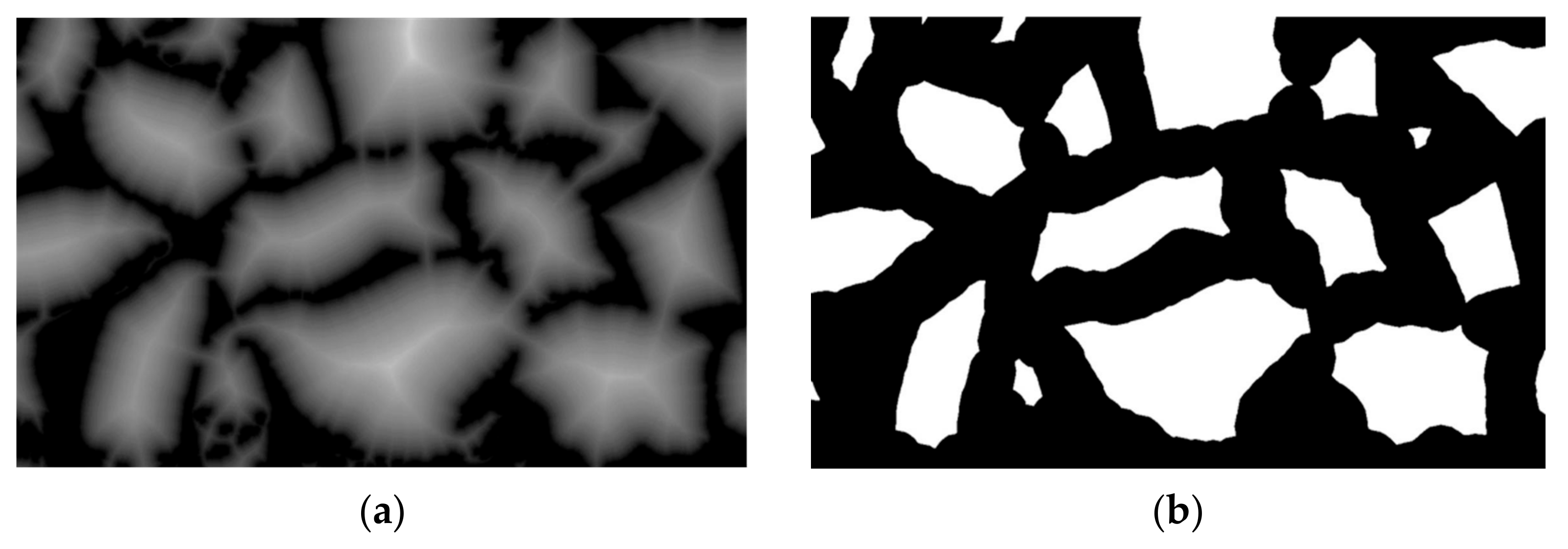
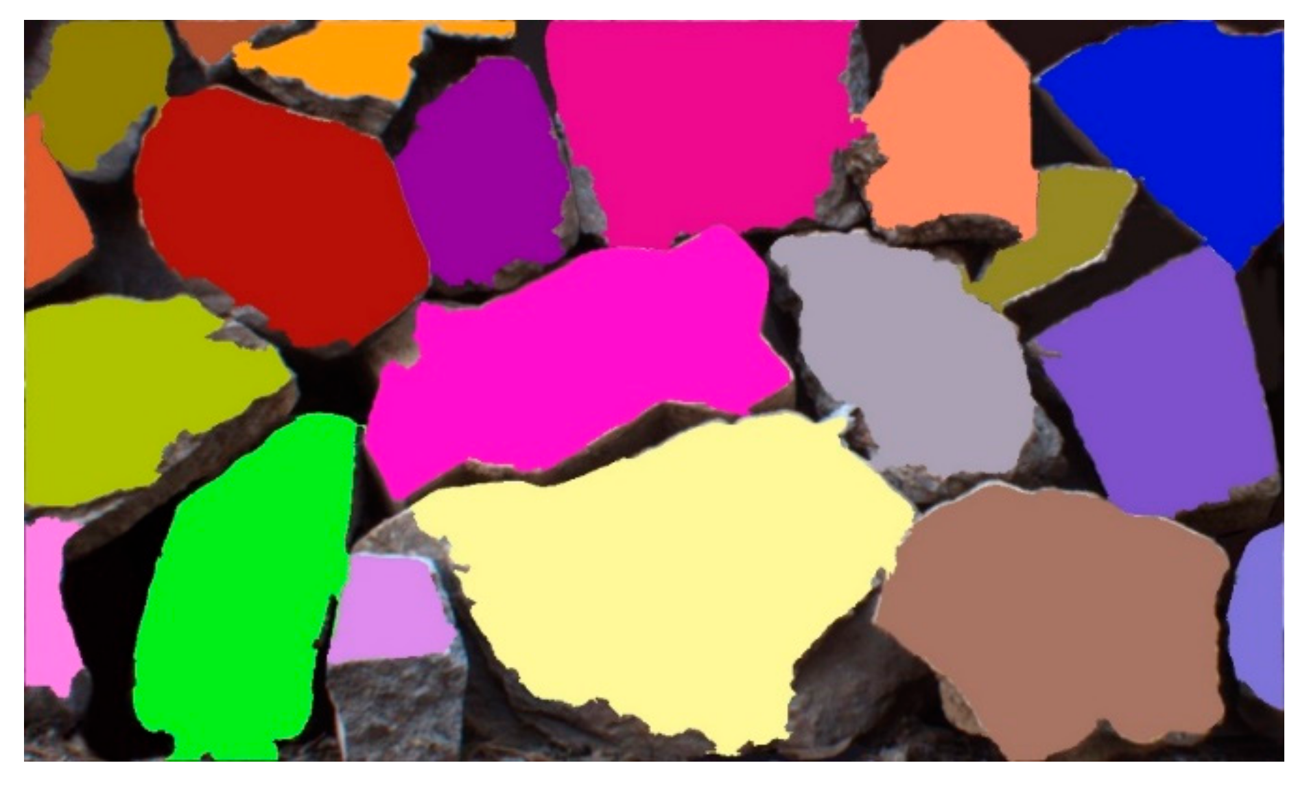
3.5. Watershed Segmentation

First, the 2D Otsu method is utilized to compute the threshold value for the preprocessed image.

$$T_{\mathrm{B}}=\lambda \times Otsu\left(I_0\right)$$

(13)

where $Otsu$ represents the 2D Otsu method, with $\lambda =0.5$ being the selected parameter. And then we employ $T_{\mathrm{B}}$ to threshold the image $I_0$ according to the following procedure:

$$\left\{\begin{array}{c}{I}_0\left(i,j\right)=255 if I_0\left(i,j\right)\ge T_{\mathrm{B}}\\ I_0\left(i,j\right)=0 if I_0\left(i,j\right)<T_{\mathrm{B}}\end{array}\right.$$

(14)

Thresholding is performed to remove a substantial portion of the background while minimizing its impact on the foreground rock blocks. Following this, small holes in the binary image are filled to mitigate their influence on the distance transformation. By extracting closed contours within the binary image and setting an area threshold, holes with enclosed contour areas smaller than the threshold are filled.

Second, the binary ore rock image undergoes a morphological opening operation to reduce the level of adhesion between different rock blocks in the ore rock image. This operation involves applying the erosion operation to the binary image A using the structural element B, followed by a dilation operation. The calculation method can be described as follows:

$$A\circ B=\left(A\mathrm{\Theta }B\right)\oplus B$$

(15)

Third, the distance transformation is conducted to compute the distance between foreground objects in a binary image and the closest background point. This operation transforms the binary image into a grayscale image that represents the corresponding distance values. Let us assume that the binary image contains a connected region with a target set $O$ and a background set $B$. The distance transformation formula for the distance map $D$ can be expressed as follows:

$$D\left(p\right)=\min \left(dis\left(p,q\right)\right), p\in O, q\in B,$$

(16)

where $dis$ represents the distance function. In this study, the fast Euclidean distance transformation algorithm utilizing a 5 × 5 template is employed. The distance transformation image $I_d$ of the ore rock binary image is depicted in Figure 4a. After thresholding, the foreground marker image is shown in Figure 4b.

Finally, the Marker Watershed algorithm is used to segment different ore rock fragments. The watershed algorithm treats the gradient image as a topographic landscape, with pixel values representing terrain heights. Local minima in the gradient image correspond to catchment basins, while the pixel maxima surrounding the minima form the watershed boundary. The watershed algorithm can generate closed contours with a single-pixel width, which greatly facilitates the computation of rock fragment sizes.

To address the issue of over-segmentation, the Marker Watershed algorithm incorporates marker control to eliminate spurious catchment basins. In this study, we refine the Marker Watershed algorithm by replacing the gradient image with the edge-enhanced SDM. The segmentation effectiveness of rock fragments using this modified Marker Watershed approach is depicted in Figure 5.

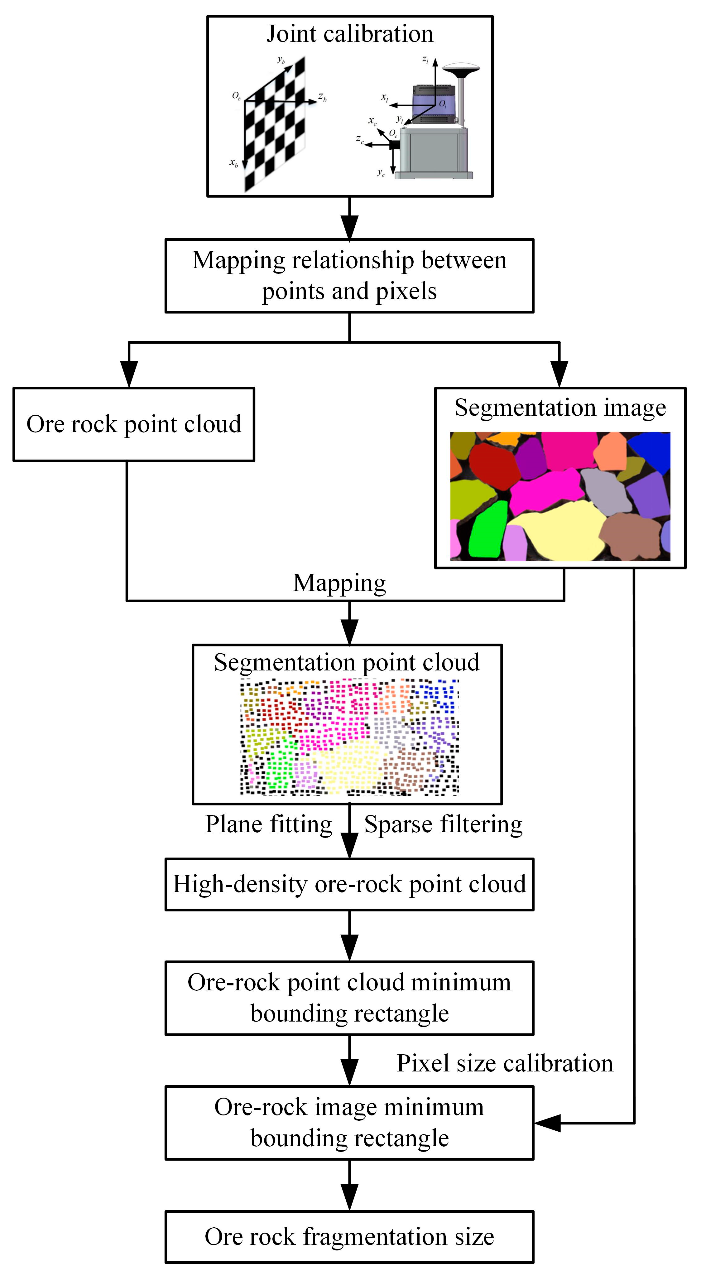
3.6. Ore Rock Fragmentation Calculation Based on Multi-Modal Calibration Mapping

The computation method for calculating the size of ore rock blocks is illustrated in Figure 6. This approach is established on the basis of a calibration mapping relationship between the point cloud and various image modalities. Initially, the rock point cloud is segmented using the information obtained from the rock segmentation image. Subsequently, the pixel size of the segmented rock image is calibrated using the characteristic size of the high-density rock block point cloud as a reference.

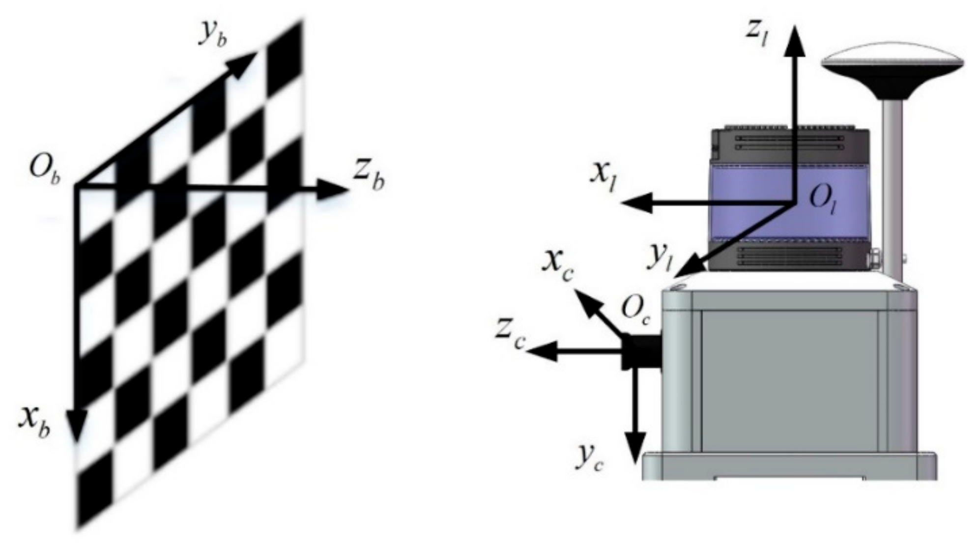
3.6.1. Calibration Mapping

The calibration mapping process between the point cloud and image is depicted in Figure 7.

The camera is internally calibrated with the use of a chessboard calibration board to obtain the camera’s intrinsic calibration matrix, denoted as $A$. Furthermore, a joint calibration is performed between the camera and the LiDAR to acquire the extrinsic calibration matrix, denoted as $[R|\mathit{t}]$. Assuming $\mathit{p}={\left[x,y,z\right]}^T$ represents an arbitrary point in the LiDAR coordinate system, $\mathit{q}={\left[u,v\right]}^T$ represents the corresponding mapped pixel in the image coordinate system, and the homogeneous coordinates of point $\mathit{p}$ and the mapped pixel $\mathit{q}$ are expressed as $\tilde{\mathit{p}}={\left[x,y,z,1\right]}^T$ and $\tilde{\mathit{q}}={\left[u,v,1\right]}^T$, respectively. Based on the pinhole camera model, the mapping relationship between $\tilde{\mathit{p}}$ and $\tilde{\mathit{q}}$ can be computed as follows:

$$s\tilde{\mathit{q}}=A\left[R|\mathit{t}\right]\tilde{\mathit{p}},$$

(17)

where $\mathit{s}$ is an arbitrary scaling factor.

The main steps involved in the joint calibration between the 3D LiDAR and the camera are outlined as follows:

(1)

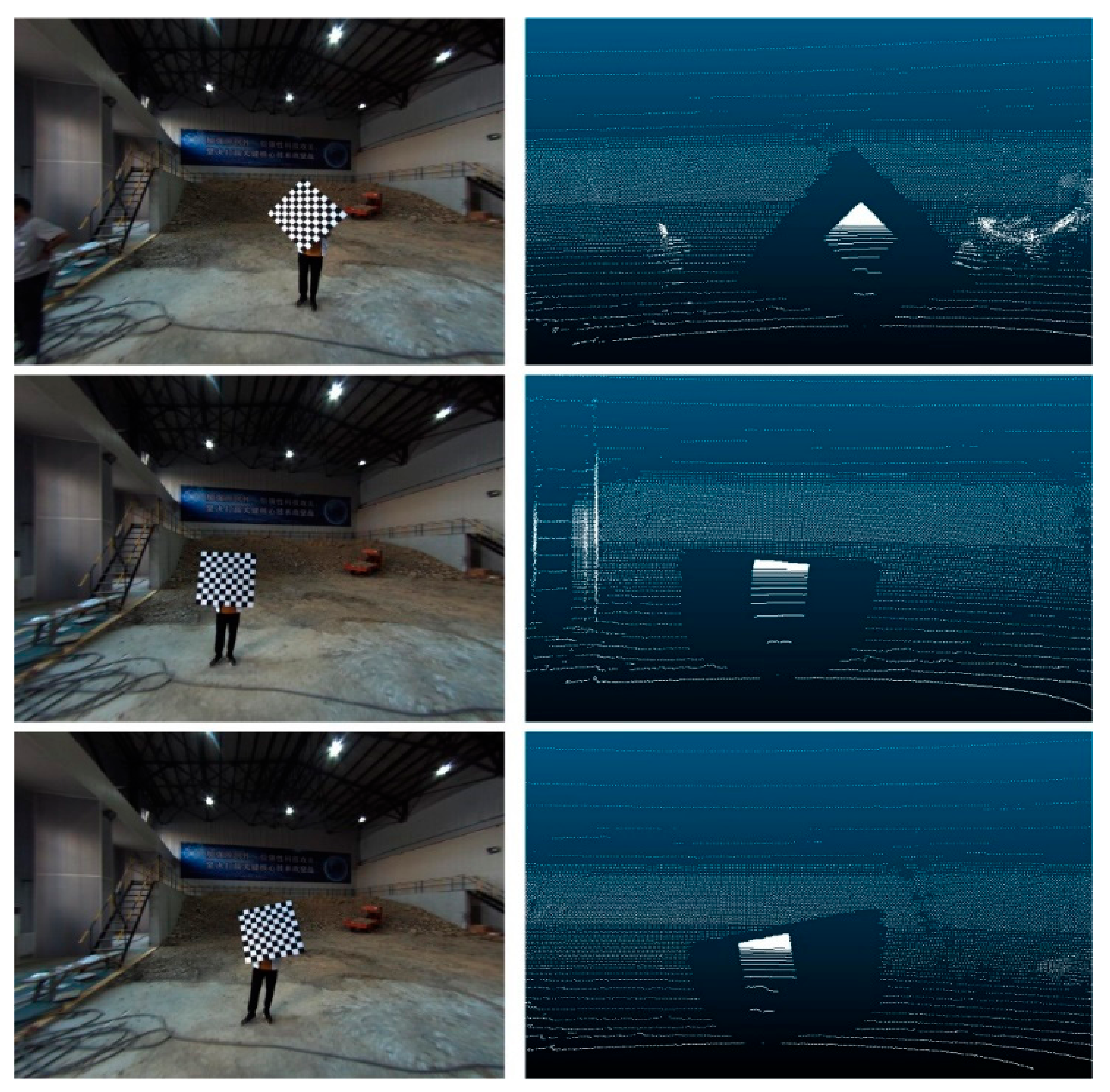
Point cloud and image data acquisition. Multiple sets of 3D LiDAR point clouds and 2D images, featuring a black and white chessboard calibration board, are captured in various poses using the 3D LiDAR and camera from a multimodal 3D environmental perception system. Figure 8 showcases the simultaneous collection results of each set of point clouds and images;

(2)

Camera intrinsic calibration. We utilize multiple sets of images, featuring a calibration board with chessboard patterns captured in different poses, to compute the camera’s intrinsic matrix using Zhang’s calibration method [24]. Simultaneously, through intrinsic calibration, we determine the positional relationship between the calibration board coordinate system and the camera coordinate system for various poses;

(3)

The extrinsic calibration of the 3D LiDAR and camera involves determining the geometric mapping relationship between the 3D point cloud and image pixels. Our research group has developed a method for calibrating the extrinsic parameters [25]. This method incorporates both line–plane and plane–plane geometric constraints to create a set of linear equations. The initial extrinsic matrix is obtained using the least squares method. Subsequently, a global error is formed by combining the pixel projection error from the camera’s intrinsic calibration and the vertical distance error of laser points resulting from the initial extrinsic calibration. To refine the calibration, this global error undergoes nonlinear global optimization based on the Levenberg–Marquardt method. Through this optimization process, the final extrinsic calibration is achieved, establishing the desired geometric mapping relationship between the 3D point cloud and image pixels.

Figure 8. Synchronization data of point clouds and images of the calibration board.

Figure 8. Synchronization data of point clouds and images of the calibration board.

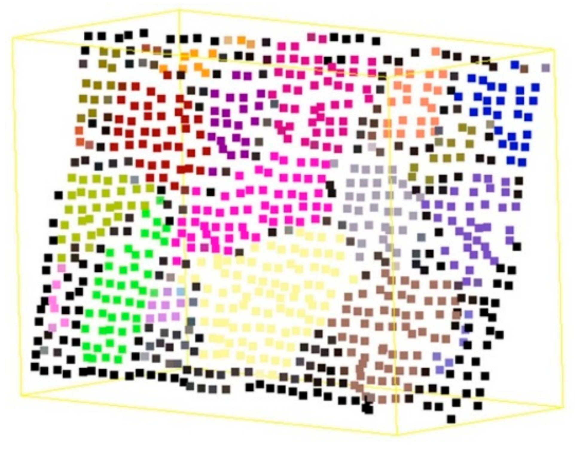
3.6.2. Point Cloud Segmentation and High-Density Ore Rock Fragments Screening

Once the calibration establishes the mapping relationship between point clouds and images, the 3D rock point clouds can be projected onto the segmented ore and rock images. This projection creates a direct correspondence between individual points and their respective pixels. Following the watershed image segmentation, different minerals in the ore image are distinguished by unique colors. By assigning the RGB values of the corresponding mineral pixels to the mapped points, the segmentation of mineral blocks in the ore point cloud can be obtained.

In the subsequent step, the Random Sample Consensus (RANSAC) algorithm is employed to fit planes to the segmented point cloud of mineral blocks. The point cloud is then projected onto these fitted planes, as depicted in Figure 9. The black points represent the background, while points of different colors correspond to different rock formations.

In order to mitigate the impact of point cloud sparsity on rock block volume calculations, it is essential to establish a suitable metric for evaluating point cloud sparsity. Furthermore, high-density rock block point clouds are filtered as reference objects for size measurements. This study evaluates the sparsity of rock block point clouds by comparing the number of points in the point cloud modality with the number of pixels in the image modality. The ratio between the point cloud point count and the image pixel count serves as an indicator for assessing the sparsity of the rock block point cloud. Sparsity analysis is conducted on all rock blocks, and they are sorted based on their sparsity levels. Finally, the three rock block point clouds with the lowest sparsity are selected as the reference objects for size measurements.

3.6.3. Pixel Size Calibration and Ore Rock Fragment Calculation

On the plane projection of the point cloud for the mining and rock segmentation, the minimum bounding rectangle is drawn around the selected high-density rock point cloud $P=\left\{P_i\right|1\le i\le 3\}$. The length $l_{p_i}$ and width $w_{p_i}$ of the rectangle are calculated based on the three-dimensional coordinates of the points. The rock block image $C=\left\{C_i\right|1\le i\le 3\}$, corresponding to the high-density rock point cloud, is identified on the rock segmentation image. The minimum bounding rectangle is drawn around each rock image, and the length $l_{c_i}$ and width $w_{c_i}$ of the rectangle are computed in pixels as the basic unit. Subsequently, the pixel size calibration of the image is performed using the characteristic dimensions of the rock point cloud. The calibration coefficient $\tau$ is determined as follows:

$$\tau =\frac{1}{6}{\displaystyle \sum _{i=1}^3\left(\frac{l_{p_i}}{l_{c_i}}+\frac{w_{p_i}}{w_{c_i}}\right)},$$

(18)

where the unit of $\tau$ is $\mathrm{cm}/\mathrm{pixel}$. Afterward, appropriate evaluation indicators for rock fragmentation are meticulously selected, and the computation and statistical analysis of rock fragmentations are carried out using the rock segmentation image.

The proposed method for pixel size calibration reduces the need for specific markers to be placed within the ore rock, making it more practical for real-world applications. In comparison with existing research methods, this approach better aligns with the requirements of practical applications. Moreover, by selecting multiple high-density rock point clouds as dimension reference objects, the robustness of the pixel calibration coefficient is greatly enhanced, thereby improving the accuracy of rock fragmentation calculations.

4. Experiments

4.1. Evaluation Metrics

We selected the equivalent diameter, the elliptical long diameter, and the elliptical short diameter as metrics to characterize the size of rock fragments. The calculation methods for these parameters are described below:

(1)

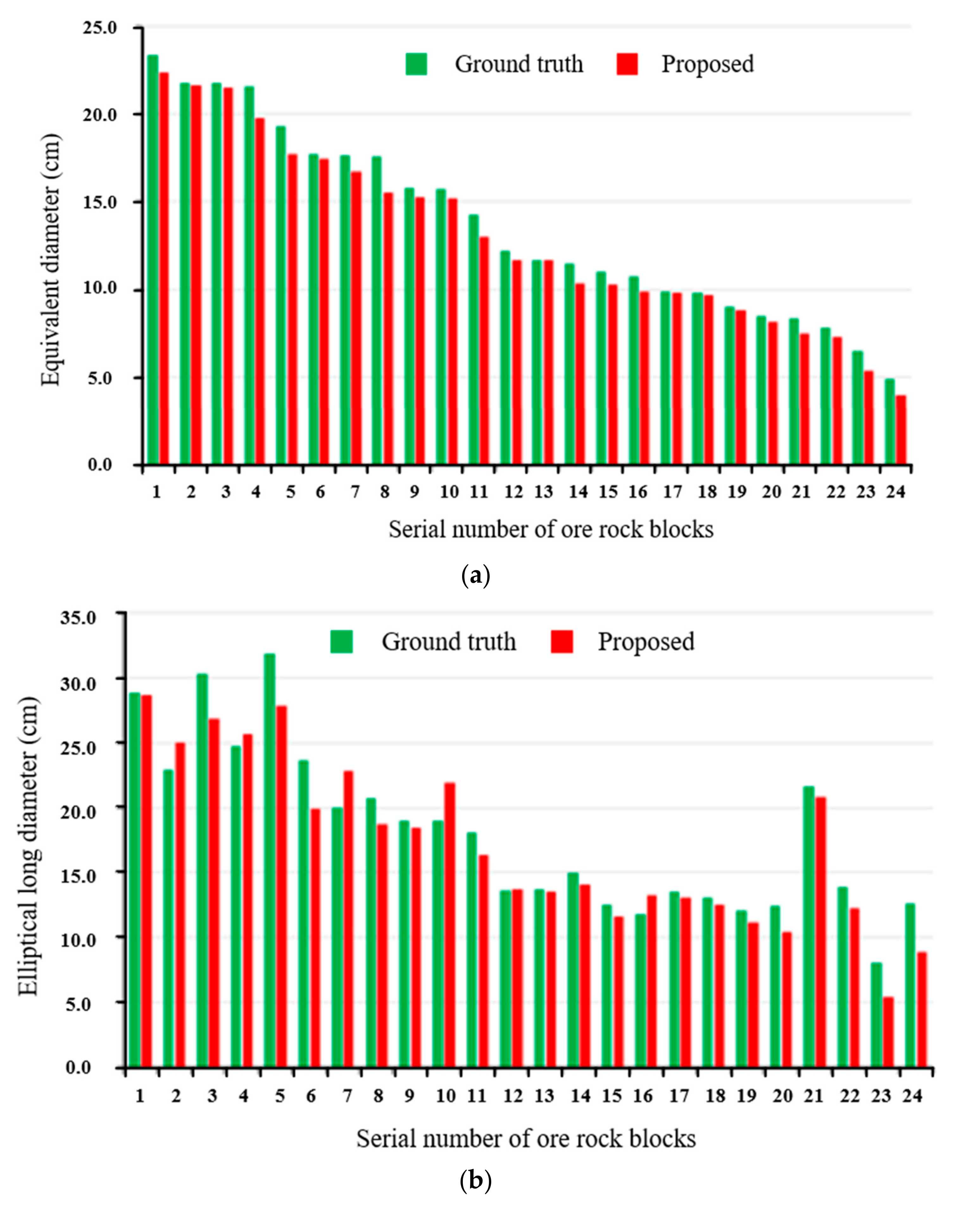
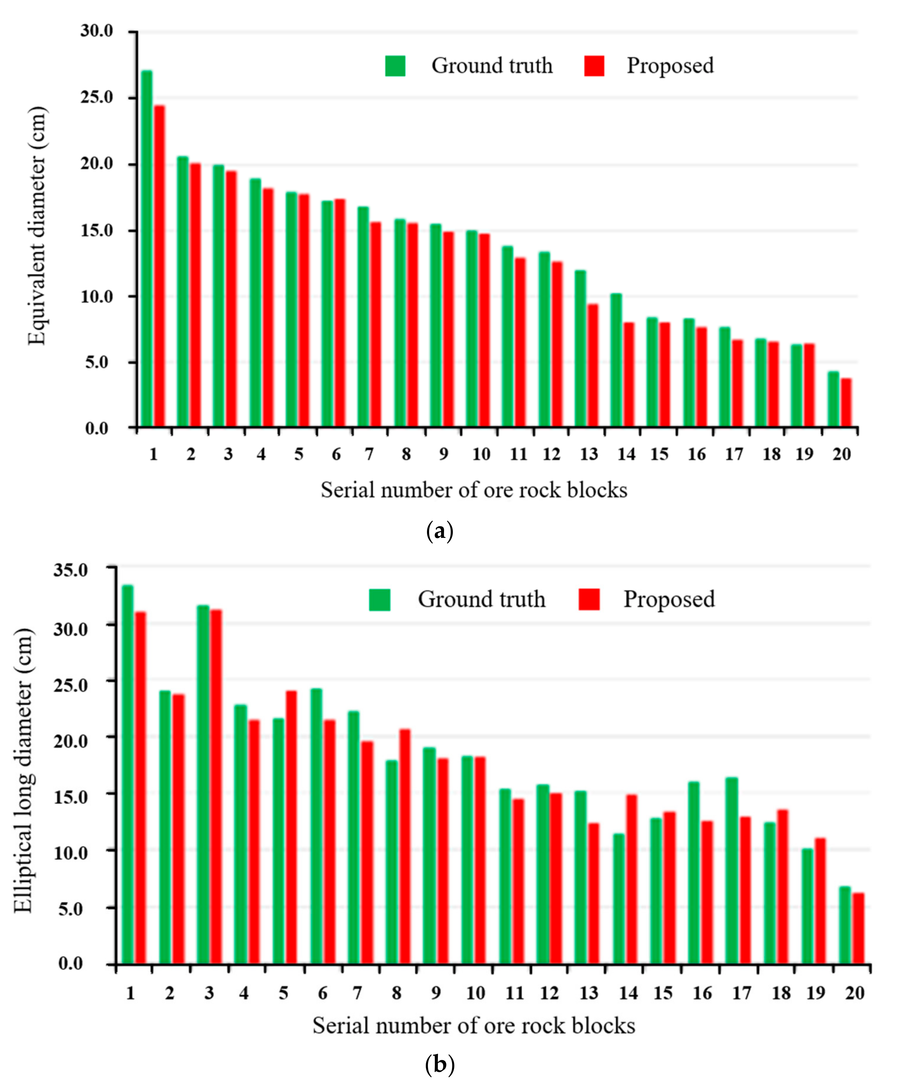
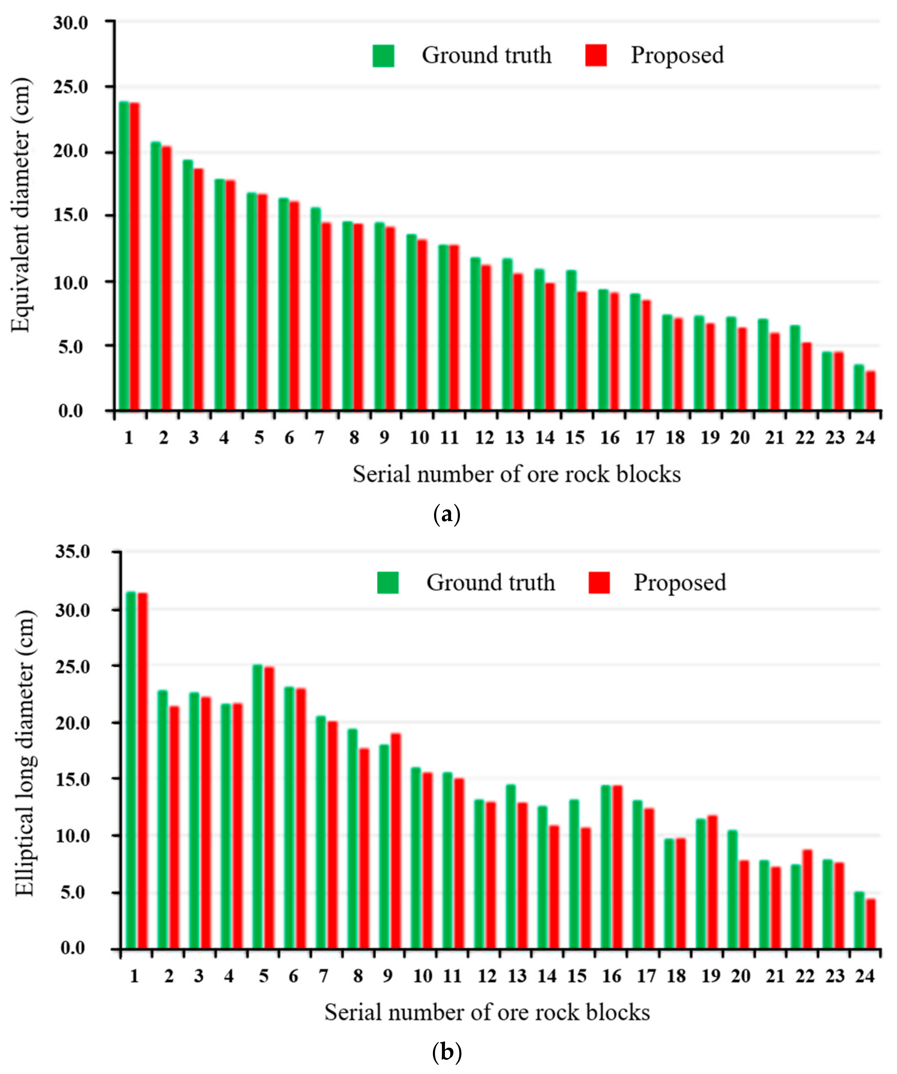
Equivalent diameter $D_E$: It is the diameter of a circle with an area that is identical to the rock block region $A$. The computational approach is as follows:

$$A=n\times \tau ,$$

(19)

$$D_E=2\sqrt{A/\pi },$$

(20)

where $n$ signifies the number of pixels contained in the rock block and $\tau$ denotes the pixel size calibration coefficient.

(2)

Elliptical long diameter $D_L$: The edge contour of the rock block is subjected to elliptical fitting, and the major axis of the fitted ellipse is represented by $D_L$. $D_L$ is the product of the pixel number $n_L$ encompassed within the major axis and the pixel calibration coefficient $\tau$. The calculation method can be summarized as follows:

$$D_L=n_L\times \tau .$$

(21)

(3)

Elliptical short diameter $D_S$: The edge contour of the rock block is subjected to elliptical fitting, and the short axis of the fitted ellipse is represented by $D_S$. $D_S$ is the product of the pixel number $n_S$ encompassed within the short axis and the pixel calibration coefficient $\tau$. The calculation method can be summarized as follows:

$$D_S=n_S\times \tau .$$

(22)

4.2. Experiments and Analysis

To verify the accuracy of the proposed method, this research conducted experimental validations using stones of different shapes and sizes in a designated laboratory. The stones were arranged in carefully designed experimental setups to accurately represent the morphology of ore and rock in the localized excavation area of the bucket. In addition, a dataset was created by simultaneously capturing rock point cloud data and image data using a three-dimensional laser scanner and an industrial camera. For the experimental validation, three sets of actual rock images and corresponding rock point clouds were selected from the dataset.

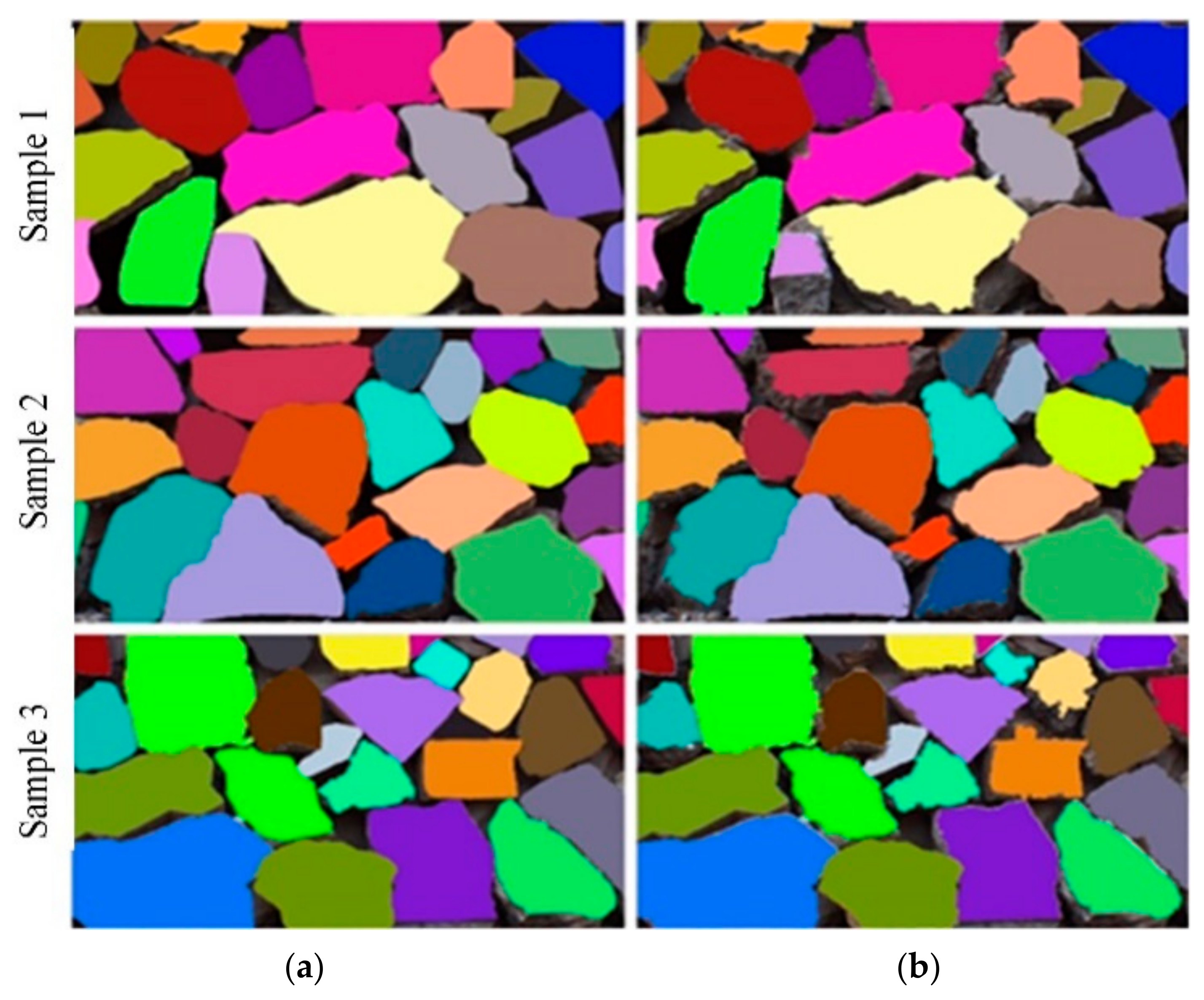
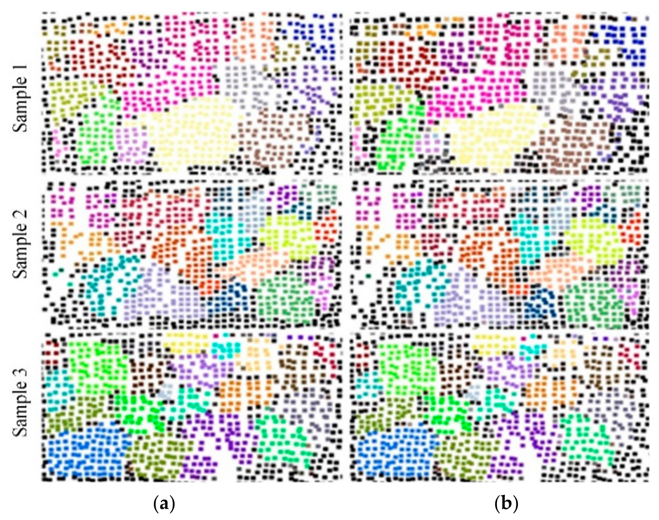
4.2.1. Visualization Segmentation Results for Ore Rock Images and Point Clouds

The rock image segmentation results proposed in this paper are presented in Figure 10a, while the ideal segmentation achieved through manual annotation is shown in Figure 10b. It can be observed that the image segmentation method effectively segmented all rock blocks and closely approximated the manually annotated ideal segmentation. This provides a solid foundation for further analysis and the calculation of rock block sizes.

After obtaining the segmentation image of the ore rocks, the ore point cloud is calibrated and mapped, resulting in the segmentation of the ore point cloud. The segmentation results of the ore point cloud using the proposed approach are depicted in Figure 11a, while the manually annotated ideal segmentation effect is shown in Figure 11b. It is evident that the segmentation results obtained from the point cloud closely resembled the manually annotated ideal segmentation of the ore blocks. This demonstrates the accuracy of the pixel size calibration by utilizing the spatial position information derived from the segmented rock point clouds.

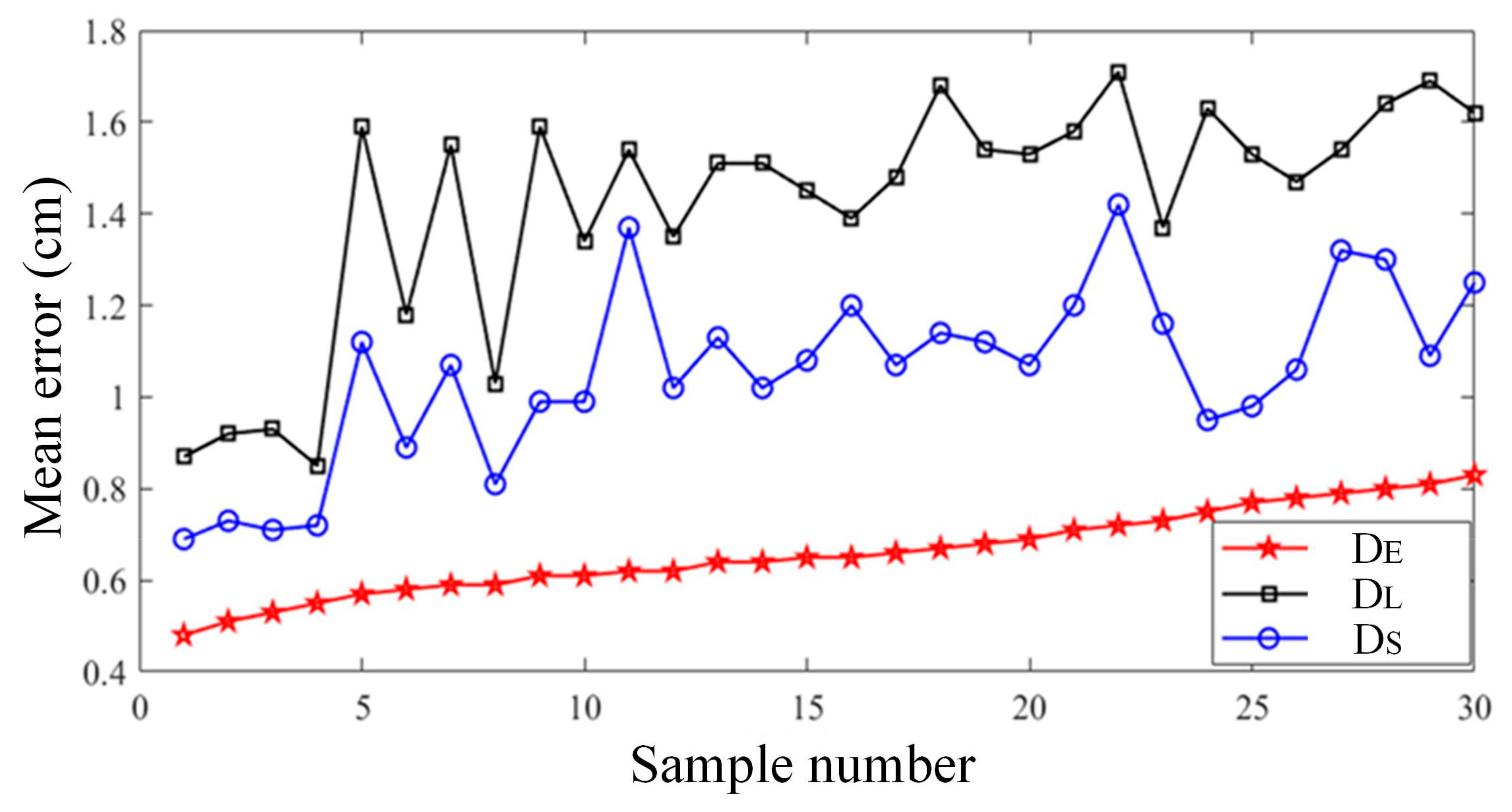
4.2.2. Quantitative Experiments

Figure 12 shows the statistical results of the equivalent diameter, elliptical long diameter, and elliptical short diameter calculation errors of ORFCM on all 30 sets of test samples.

It can be found that the calculation error of the equivalent diameter was the smallest among the three evaluation indicators, with an average error value of 0.66 cm on all test samples; the second was the elliptical short diameter, which had an average error value of 1.06 cm on all test samples; finally, the elliptical long diameter had an average error value of 1.42 cm on all test samples. Experiments demonstrate that the multimodal fusion method for calculating rock fragmentation proposed in this article had relatively small computational errors in all three evaluation indicators and could effectively meet the practical needs of intelligent mining electric shovels for calculating rock fragmentation.

Furthermore, we selected three samples to present the experimental results in more detail by using the equivalent diameter and the elliptical long diameter as the metrics. The computed results for the size of rock blocks in Sample I are presented in Figure 13.

Figure 13a shows the histogram of the equivalent diameters for all rock blocks in Sample I. It can be observed that the difference between the equivalent diameters of rock blocks and the ideal values was minimal, with an average error of 0.7 cm for all rock blocks. Figure 13b displays the histogram of the major axes for all rock blocks in Sample I. Upon close examination of the data, it is evident that the disparity between the major axes of rock blocks and the ideal values was negligible, with an average discrepancy of only 1.7 cm for all rock blocks.

Figure 14 presents the computed results of rock block size for Sample II. Figure 14a displays the histogram of the equivalent diameters for all rock blocks in Sample II. The obtained equivalent diameters of ore rock blocks exhibited minimal disparity with the ideal values, with an average error of 0.8 cm for all rock blocks. The statistical histogram of the major axes for all rock blocks in Sample II is shown in Figure 14b, indicating a slight variation in the elliptical major axis of the rock blocks compared with the ideal values. The average error in the elliptical major axis of all rock blocks is 1.7 cm.

The rock block computation results for Sample III are shown in Figure 15. In Figure 15a, the histogram illustrates the statistical distribution of equivalent diameters for all rock blocks in Sample III. ORFCM accurately determines the rock block equivalent diameters, with an average difference of only 0.5 cm compared with the ideal values across all rock blocks. Figure 15b presents the statistical histogram of major axes for the rock blocks in Sample III. It is evident that ORFCM achieved minimal deviation from the ideal values in terms of rock block major axes, with an average difference of 0.9 cm among all rock blocks.

4.2.3. Comparative Experiments

A comparative experiment was carried out to verify the performance of our method compared with existing works [3,6,21] in terms of the mean errors of D_E, D_L, and D_S. Among them, Refs. [3,6] are based on the image modality for ore rock fragmentation calculation. Ref. [21] is based on the point cloud modality for ore rock fragmentation calculation.

Table 1. Statistics of the calculation errors in the comparative experiments.

Method	Mean Error of DE (cm)	Mean Error of DL (cm)	Mean Error of DS (cm)
Our method	0.66	1.42	1.06
[3]	0.85	1.94	1.87
[6]	0.68	1.52	1.08
[21]	0.93	1.68	1.92

shows the experimental results of different methods.

From Table 1, we can see that our method performed best in terms of the mean errors of D_E, D_L, and D_S. Among all the comparison methods, Ref. [21] performed the worst, mainly due to the low resolution of point clouds obtained by LiDAR, which made it difficult to accurately calculate the block size of fine-grained ore rocks. Compared with our method, Refs. [3,6] did not perform as well in solving the problem of image under-segmentation caused by blurry edges as our method.

4.2.4. Ablation Experiments

The ablation experiment was conducted to verify the important role of the two key technologies, SDM and multi-scale adaptive edge detector, in the proposed method. The experimental control groups were set up as follows: (1) using the gradient map instead of SDM to compare and (2) selecting edge-detection algorithms, such as Canny [26], Edge Drawing [27], and SBED [28], to replace the multi-scale adaptive edge detector.

Table 2. Statistics of the calculation errors in the ablation experiments.

Method	Mean Error of DE (cm)	Mean Error of DL (cm)	Mean Error of DS (cm)
Our method	0.66	1.42	1.06
Gradient map	1.09	2.87	2.31
Canny	0.97	2.53	1.94
Edge drawing	0.84	2.24	1.76
SBED	0.76	1.96	1.61

shows the statistics of the average errors of the equivalent diameter, elliptical major diameter, and elliptical short diameter of our method and the comparison methods for all test samples. Through observation, it can be seen that the mean errors of the equivalent diameter, elliptical major diameter, and elliptical short diameter all increased to varying degrees after replacing SDM with the gradient map. Among them, the mean error of the equivalent diameter increased by 0.43 cm, the mean error of the elliptical long diameter increased by 1.45 cm, and the mean error of the elliptical short diameter increased by 1.25 cm. The experiments demonstrate that SDM can improve the accuracy of ore rock fragmentation calculation.

It also can be seen that the mean errors of the equivalent diameter, elliptical major diameter, and elliptical short diameter increased to varying degrees after replacing the multi-scale adaptive edge detector with Canny, Edge Drawing, and SBED. Among them, Canny had a significant increase in error, with a mean error of 0.31 cm in the equivalent diameter, 1.11 cm in the elliptical long diameter, and 0.88 cm in the elliptical short diameter. The experiments demonstrate that multi-scale adaptive edge detector can improve the accuracy of the ore rock fragmentation calculation.

4.2.5. Discussion

The reasons that our method can achieve good performance in the experiments are mainly due to the following aspects: (1) through multimodal fusion, the size of image pixels is calibrated by using the spatial position information of the point cloud, which effectively solves the problem that a single mode cannot accurately calculate the ore rock fragmentation; and (2) through the construction of the standard deviation map and multi-scale adaptive edge detection, the marked watershed image segmentation algorithm was improved, effectively solving the problem of image under-segmentation.

5. Conclusions

To solve the problem that the single mode of an image or point cloud cannot accurately calculate the ore rock fragmentation, this paper proposes a calculation method for ore rock fragmentation based on the point cloud and image multi-mode fusion. The main contributions are summarized as follows:

(1)

Aiming at the problem that a single mode cannot accurately calculate the ore rock fragmentation, a multi-mode fusion algorithm was proposed, which used the spatial position information of the point cloud to calibrate the size of image pixels, and accurately achieved ore rock fragmentation calculation without relying on external markers to calibrate the pixel size;

(2)

To solve the problem of image under-segmentation caused by weak edges, the construction of the standard deviation map and multi-scale adaptive edge detection had effectively enhanced weak edges. This achieved an improvement in the marked watershed image segmentation algorithm and improved the accuracy of image segmentation;

(3)

Experiments demonstrated that the proposed method could accurately calculate the fragmentation of ore rock blocks with different morphologies in the local excavation area of the bucket. The average error of the equivalent diameter of ore rock blocks was 0.66 cm, the average error of elliptical long diameter was 1.42 cm, and the average error of elliptical short diameter was 1.06 cm, which could effectively meet practical engineering needs.

The ore rock fragmentation calculation method proposed in this paper gives full play to the advantages of point cloud and image multi-mode fusion, effectively overcomes the shortcomings of the ore rock fragmentation calculation method based on a single mode, and improves the accuracy of ore rock fragmentation calculation and the practicability of the algorithm, which is of great significance for improving the reliability of intelligent mining shovel autonomous mining operations and reducing the failure rate of equipment.

References

- Siddiqui, F.; Ali, S.; Behan, M. Measurement of size distribution of blasted rock using digital image processing. Eng. Sci. 2009, 20, 81–93. [Google Scholar] [CrossRef]
- Si, L.; Wang, Z.B.; Liu, P.; Tan, C.; Chen, H.; Wei, D. A Novel Coal-Rock Recognition Method for Coal Mining Working Face Based on Laser Point Cloud Data. IEEE Trans. Instrum. Meas. 2021, 70, 2514118. [Google Scholar] [CrossRef]
- Amankwah, A.; Aldrich, C. Automatic ore image segmentation using mean shift and watershed transform. In Proceedings of the 21st International Conference Radioelektronika 2011, Brno, Czech Republic, 19–20 April 2011; pp. 1–8. [Google Scholar]
- Zhang, G.; Li, M.; Zhan, Y. Ore image thresholding segmentation using double windows with fisher discrimination. In Proceedings of the 2017 13th International Conference on Natural Computation, Fuzzy Systems and Knowledge Discovery (ICNC-FSKD), Guilin, China, 29–31 July 2017; pp. 18–25. [Google Scholar]
- Wang, R.; Zhang, W.; Shao, L. Research of Ore Particle Size Detection Based on Image Processing; Springer: Singapore, 2018; pp. 505–514. [Google Scholar]
- Guo, Q.P.; Wang, Y.C.; Yang, S.J.; Xiang, Z.B. A method of blasted rock image segmentation based on improved watershed algorithm. Sci. Rep. 2022, 12, 7143. [Google Scholar] [CrossRef]
- Ding, X.; Zhou, W.; Lu, X. Distribution characteristics of fragments size and optimization of blasting parameters under blasting impact load in open-pit mine. IEEE Access 2019, 7, 137501–137516. [Google Scholar] [CrossRef]
- Wang, W.; Bergholm, F. Fragment size estimation without image segmentation. Imaging Sci. J. 2007, 56, 91–96. [Google Scholar] [CrossRef]
- Liu, Y.; Sun, J.H.; Yu, H.Y.; Wang, Y.Y.; Zhou, X.K. An Improved Grey Wolf Optimizer Based on Differential Evolution and OTSU Algorithm. Appl. Sci. 2020, 10, 6343. [Google Scholar] [CrossRef]
- Zhang, G.; Liu, G.; Zhu, H. Ore image thresholding using bi-neighbourhood Otsu’s approach. Electron. Lett. 2010, 46, 1–3. [Google Scholar] [CrossRef]
- Hadi, Y.; Hamid, M.; Mohammad, A. Determining the fragmented rock size distribution using textural feature extraction of images. Powder Technol. 2019, 342, 630–641. [Google Scholar]
- Xie, C.; Nguyen, H.; Bui, X.N. Predicting rock size distribution in mine blasting using various novel soft computing models based on meta-heuristics and machine learning algorithms. Geosci. Front. 2021, 12, 35–42. [Google Scholar] [CrossRef]
- Yuan, L.; Duan, Y. A Method of Ore Image Segmentation Based on Deep Learning; Springer: Cham, Switzerland, 2018; pp. 508–519. [Google Scholar]
- Ko, Y.; Shang, H. A neural network-based soft sensor for particle size distribution using image analysis. Powder Technol. 2011, 212, 359–366. [Google Scholar] [CrossRef]
- Shubham, S.; Debasis, D.; Sudipta, B. Prediction of particle size distribution curves of dump materials using convolutional neural networks. Rock Mech. Rock Eng. 2021, 21, 15–24. [Google Scholar]
- He, K.; Gkioxari, G.; Dollár, P. Mask r-cnn. In Proceedings of the IEEE International Conference on Computer Vision, Venice, Italy, 22–29 October 2017. [Google Scholar]
- Xiao, D.; Liu, X.; Le, B. An ore image segmentation method based on RDU-Net model. Sensors 2020, 17, 4979. [Google Scholar] [CrossRef]
- Jin, Q.; Meng, Z.; Pham, T. DUNet: A deformable network for retinal vessel segmentation. Knowl.-Based Syst. 2019, 178, 149–162. [Google Scholar] [CrossRef]
- Matthew, J. Automated image segmentation and analysis of rock piles in an open-pit mine. In Proceedings of the 2013 International Conference on Digital Image Computing: Techniques and Applications (DICTA), Hobart, TAS, Australia, 26–28 November 2013. [Google Scholar]
- Onederra, I.; Thurley, M.; Catalan, A. Measuring blast fragmentation at Esperanza mine using 3D laser scanning. Min. Technol. 2015, 124, 34–46. [Google Scholar] [CrossRef]
- Campbell, A.; Thurley, M. Application of laser scanning to measure fragmentation in underground mines. Min. Technol. 2017, 126, 240–247. [Google Scholar] [CrossRef]
- Engin, I.; Maerz, N.; Boyko, K. Practical measurement of size distribution of blasted rocks using LiDAR scan data. Rock Mech. Rock Eng. 2020, 53, 4653–4671. [Google Scholar] [CrossRef]
- Cui, Y.H.; An, Y.; Sun, W.; Hu, H.S.; Song, X.G. Multiscale adaptive edge detector for images based on a novel standard deviation map. IEEE Trans. Instrum. Meas. 2021, 70, 5010913. [Google Scholar] [CrossRef]
- Zhang, Z. A flexible new technique for camera calibration. IEEE Trans. Pattern Anal. Mach. Intell. 2000, 22, 1330–1334. [Google Scholar] [CrossRef]
- An, Y.; Li, B.; Wang, L. Calibration of a 3D laser rangefinder and a camera based on optimization solution. J. Ind. Manag. Optim. 2021, 17, 427–445. [Google Scholar] [CrossRef]
- Canny, J. A computational approach to edge detection. IEEE Trans. Pattern Anal. Mach. Intell. 1986, 8, 679–698. [Google Scholar] [CrossRef]
- Topal, C.; Akinlar, C. Edge drawing: A combined real-time edge and segment detector. J. Vis. Commun. Image Represent. 2012, 23, 862–872. [Google Scholar] [CrossRef]
- Zhang, H.; Wu, C.; Zhang, L. A novel centroid update approach for clustering-based superpixel methods and superpixel-based edge detection. In Proceedings of the 2020 IEEE International Conference on Image Processing (ICIP), Abu Dhabi, United Arab Emirates, 25–28 October 2020. [Google Scholar]