Proactive Service Caching in a MEC System by Using Spatio-Temporal Correlation among MEC Servers

Abstract

Optimizingthe cache hit rate in a multi-access edge computing (MEC) system is essential in increasing the utility of a system. A pivotal challenge within this context lies in predicting the popularity of a service. However, accurately predicting popular services for each MEC server (MECS) is hindered by the dynamic nature of user preferences in both time and space, coupled with the necessity for real-time adaptability. In this paper, we address this challenge by employing the Convolutional Long Short-Term Memory (ConvLSTM) model, which can capture both temporal and spatial correlations inherent in service request patterns. Our proposed methodology leverages ConvLSTM for service popularity prediction by modeling the distribution of service popularity in a MEC system as a heatmap image. Additionally, we propose a procedure that predicts service popularity in each MECS through a sequence of heatmap images. Through simulation studies using real-world datasets, we compare the performance of our method with that of the LSTM-based method. In the LSTM-based method, each MECS predicts the service popularity independently. On the contrary, our method takes a holistic approach by considering spatio-temporal correlations among MECSs during prediction. As a result, our method increases the average cache hit rate by more than $6.97\%$ compared to the LSTM-based method. From an implementation standpoint, our method requires only one ConvLSTM model while the LSTM-based method requires at least one LSTM model for each MECS. Thus, compared to the LSTM-based method, our method reduces the deep learning model parameters by 32.15%.

1. Introduction

Online mobile services are evolving from traditional information searching and retrieval towards innovative artificial intelligence (AI)-based services. This transformative shift encompasses a spectrum of functionalities, including language translation, image recognition, autonomous driving, artificial intelligence of things (AIoT), and augmented reality/virtual reality [1,2]. The advent of these advanced services not only necessitates substantial computing power and data but also demands the swift delivery of results to end users. The prevalent cloud computing service paradigm has been instrumental in supporting computationally intensive services [3,4]. However, a common challenge arises due to the considerable distance between end users and cloud servers. Furthermore, the escalating volume of service requests contributes to heightened congestion levels in the backhaul network. Consequently, while the cloud computing service paradigm provides significant computing power and extensive storage to end users, it encounters challenges in meeting the service delay requirements of AI-based services [5,6]. In response to this challenge, the Multi-Access Edge Computing (MEC) system has emerged [7,8]. In the MEC system, a cluster of MEC servers (MECSs) strategically positions itself in proximity to end users. This strategic placement enables users to offload computing-intensive and delay-sensitive tasks to the nearest MECS. Subsequently, the MECS processes these tasks and transmits the results back to the users. By bringing servers into close proximity to users, the MEC system effectively mitigates service delays and alleviates the strain on the backhaul network.

In the realm of MEC system design, a pivotal challenge lies in the task offloading decision problem. Various task offloading methods have been proposed [9,10], generally falling into two primary categories. The first group involves users making intelligent offloading decisions, aiming to optimize service delay and the energy required for service completion [11,12]. Conversely, another research strand focuses on MEC system operators striving to optimize the utilization of computing and communication resources while ensuring users experience reasonable service delays [13,14]. However, these approaches often overlook the crucial aspect of service availability for the offloaded tasks. Essentially, they assume that services requested by tasks offloaded from users to the MECS are always available at the MECS. However, due to the inherent limitations of MECS in terms of computing power and storage compared to cloud servers, it can only accommodate a subset of the services available on cloud servers. Consequently, if MECS lacks the service requested by the offloaded task, it must fetch the service from the cloud server. Given that the installation and loading of services on MECS entail time, the effective management of service caching emerges as a critical factor in mitigating service delays within the MEC system.

Ensuring the inclusion of the most popular services in each MECS cache is important in achieving a higher cache hit rate. The popularity of services within MECS is intricately linked to the service preferences of users in the respective MECS service area. The dynamic nature of user mobility causes changes in the set of users within the MECS service area over time. Moreover, user service preferences evolve over time as well. Consequently, determining the optimal service set to be cached in a specific MECS within the MEC system presents a significant challenge. To address this challenge, popularity prediction methods have been proposed [15,16]. These methods delve into diverse metrics for each service, scrutinize their changing patterns, and extrapolate the future popularity of each service. By leveraging these identified patterns, they make estimates about the future popularity of each service. However, these methods primarily rely on the temporal relationships among services within individual MECS to forecast service popularity. Since users change locations over time, not only the users currently residing in the service area of a MECS but also the users served by the neighboring MECSs affect the future service popularity in the MECS. Consequently, integrating the spatial–temporal correlations between MECS enhances the accuracy of service popularity predictions. From an implementation standpoint, the number of predictors required in these popularity prediction methods escalates with the expansion of services and MECSs. Thus, concerns about scalability may surface as the MEC system grows.

In response to the identified challenges, we propose a proactive service caching methodology inspired by the Convolutional Long Short-Term Memory (ConvLSTM) model, recognized for its efficacy in video frame prediction [17,18]. Our approach seeks to exploit the inherent spatio-temporal relationships among service popularity within a MEC system. To operationalize the ConvLSTM model for this purpose, we discretize time into time slots and construct a heatmap that collectively depicts the distribution of service popularity in each MECS during a given time slot. Treating each heatmap in a time slot as a frame, we conceptualize the sequence of heatmaps as a video. Subsequently, we train a ConvLSTM model to predict the upcoming heatmap based on a few recent heatmaps. At the beginning of each time slot, we leverage the trained model to identify the most popular services from the predicted heatmap. These services are then selected to be cached on each MECS for the ensuing time slot. Utilizing a heatmap containing the popularity of each service across MECS as input enables us to comprehensively predict the popularity of all services in all MECS simultaneously. This holistic approach contributes to an enhanced service cache hit rate in each MECS. In addition, our methodology stands out by requiring only a single predictor model, as opposed to conventional methods necessitating separate prediction models for each service and MECS. This consolidation not only streamlines the predictive process but also significantly improves the scalability of a MEC system. Our main contributions can be summarized as follows.

• We propose a framework for proactive service caching by taking a deep learning approach. Inspired by the ConvLSTM model that successfully predicts video frames by exploiting the hidden spatio-temporal relationships in the frames, we incorporate the ConvLSTM model as a fundamental element in our proactive service caching methodology.
• We propose a procedure that utilizes ConvLSTM model for accurately predicting service popularity for each MECS over time. We construct heatmaps collectively representing the distribution of service popularity in a MEC system during each time slot. Treating each heatmap in a time slot as a frame, we conceptualize the sequence of heatmaps as a video. We predict the next heatmap by using the ConvLSTM model and identify the most popular services for the upcoming time slot from the predicted heatmap.
• Through simulation studies using real-world datasets, we verify that our method outperforms conventional LSTM-based method in terms of the cache hit rate and the amount of model parameters required to predict service popularity in a MEC system.

The rest of the paper is organized as follows. In Section 2, we discuss the related works. We explain the system model and formalize the problem in Section 3. In Section 4, we present our proactive caching strategy. In Section 5, we verify the proposed method by comparing its performance with that of the conventional method through simulation studies using real-world datasets. We conclude the paper with future research directions in Section 6. Before we proceed, in

Table 1. Notations used.

Notation	Meaning
$\mathcal{M}=\{1,\dots M\}$	A set of MECS in a MEC system
$\mathcal{K}=\{1,\dots K\}$	A set of services provided by a MEC system
${\eta }_m$	Service cache size of MECS m
$a_{m,k}\left(t\right)$	1: a service k is cached at MECS m during a time slot t, 0: otherwise.
$A_{M\times K}\left(t\right)$	Service cache state of a MEC system during a time slot t
$S_m\left(t\right)$	A set of services cached at MECS m during a time slot t
$U_m\left(t\right)$	A set of users in the service area of MECS m during a time slot t
$b_{m,u,k}\left(t\right)$	1: a service k requested by user u is at MECS m during a time slot t. 0: otherwise
$f_{m,k}\left(t\right)$	popularity of a service k in MECS m during a time slot t
$F_{M\times K}\left(t\right)$	service popularity matrix of a MEC system during a time slot t
$w_a$	the number of recent past heatmap images used for prediction
$b_{m,k}\left(t\right)$	the number of times MECS m receives the request of service k during a time slot t
$Z_m\left(t\right)$	the set of $b_{m,k}\left(t\right)$s at a MECS m ($\forall k\in \mathcal{K}$)
${\nu }_{m,k}\left(t\right)$	$f_{m,k}\left(t\right)$ normalized by $f_m^M\left(t\right)=ma{x}_{k\in \mathcal{K}}\left(f_{m,k}\left(t\right)\right)$
$\mathsf{\Omega }\left(t\right)$	a heatmap image of a MEC system at the end of a time slot t
$\widehat{\mathsf{\Omega }}\left(t\right)$	predicted heatmap image of a MEC system at the start of a time slot t
${\delta }_{m,k}\left(t\right)$	popularity prediction error for a service k at MECS m during a time slot t
$a_m\left(t\right)$	service cache similarity degree at MECS m during a time slot t
${\rho }_m\left(t\right)$	relative service cache hit rate at MECS m during a time slot t

, we present the notations used in this paper.

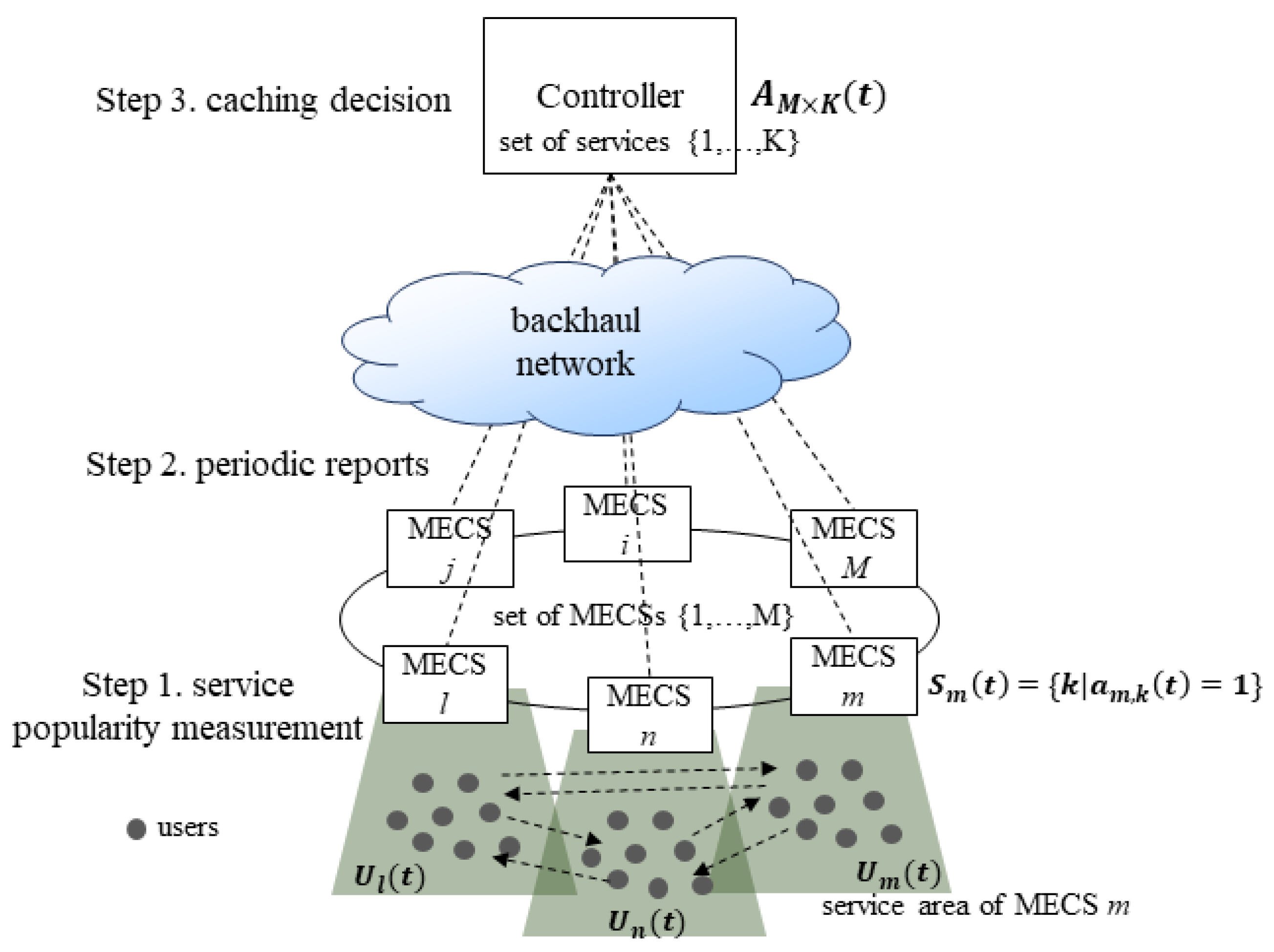
2. Related Works

2.1. Caching in a MEC System

Various cache management methods have been proposed for a MEC system. In [19,20], a game-theoretic approach is taken for making a caching decision. After modeling the interaction between a MECS and wireless devices as a two-stage Stackelberg game under incomplete information, the authors in [19] devise two strategies for the game. The first strategy is used for a MECS to make the caching and the price decision. The second strategy is used for a wireless device to make a task offloading decision. A stochastic differential game is used in [20] to formulate a dynamic cache control problem. Since the computational complexity of the problem is huge, both the mean-field game theory and the stochastic-geometry are used to transform the original problem into a more tractable form. Then, authors propose an iterative algorithm for optimal caching control. However, these game-theoretic methods require information exchange among the players. Thus, the control overhead increases in proportion to the number of devices and the number of MECSs. In addition, they require an iterative process to reach an equilibrium state. Therefore, they cannot make a decision until the iterative process converges nor adapt quickly to topology changes.

In [21], a service cache placement problem and a task offloading problem are jointly investigated. The joint problem is formulated as an average service response time minimization problem with a long-term energy consumption constraint. To resolve the problem without unknown future information, an online algorithm is devised by using the Lyapunov optimization framework and deep reinforcement learning (DRL). DRL-based methods are also proposed in [22,23]. The authors in [22] propose a cooperative video caching method for a MEC system by combining the knowledge graph (KG) and DRL. The KG is used to determine a set of candidate videos by inferrinIn [23], a model-free reinforcement learning algorithm called RL-Cache is proposed to decide whether or not to accept a requested object into the content distribution network’s cache. RL-Cache uses the size, frequency, and request recency of an object as an input feature for a feed-forward neural network that determines the admission probability of an object. However, these DRL-based methods do not exploit the spatio-temporal relation among the cached services in each MECS. In addition, they are reactive in that they make a caching decision in an on-demand manner. In [24], the authors analyze the road side unit (RSU) historical content request data and calculate the spatial–temporal correlation among the RSUs in terms of the request number, which is used to predict the service popularity in each RSU. They also employ multi-agent RL (MARL) to cope with the diversity of the popularity. However, unlike the method in [24] that uses a traditional statistical tool to directly calculate the correlation, we adopt a deep learning model to use the hidden features in the spatio-temporal relationships.

To make a caching decision in a proactive manner, the dynamics of service popularity is often considered as a time series, and a deep learning model that can handle sequential data is adopted to predict the future service popularity. An LSTM encoder and decoder model is used in [25] to map a sequence of objects requested so far to the top-k objects most likely to be requested in the future. In [26], a two-step model is proposed. In the first step, the popularity of a video genre in a future time slot is predicted. Then, the popularity of a video belonging to the prevalent genre in the same time slot is further predicted in the second step. An LSTM model is also used in [27]. The authors predict the number of content requests by the seq2seq LSTM model. Using the priority of the content and predicted popularity, they solve the cache placement problem with the binary particle swarm optimization (BPSO) technique. However, since BPSO is an iterative process, it takes time to find a solution.

Attention-based methods have been proposed for a caching problem in a MEC system. In [15], the authors propose a multi-head attention-based popularity prediction model (MAPP). After proposing an architecture that integrates MEC in social content-centric network, they use MAPP to predict content popularity by considering the history of content popularity, social relationships, and geographic location. However, they mainly use temporal correlations in the data when predicting the popularity. A transformer-based edge (TEDGE) caching scheme based on the attention-based vision transformer (ViT) is proposed in [28]. At the end of each time window, they aim to determine the top-k popular contents in the future by directly mapping the request patterns of all contents during the current time window to their future request patterns. In [29], authors improve the TEDGE by proposing a self-supervised caching scheme called CoPo. CoPo distinguishes the input samples by utilizing the contrastive learning paradigm. Since CoPo does not need all the input request patterns of all the contents at the same time, it can reduce the algorithm complexity, and even the number of contents increases. In addition, CoPo does not require manual labeling for model training. In [30], a parallel ViT with cross attention (ViT-CAT) fusion is proposed, which is composed of two ViT networks. The first ViT network collects the temporal correlation of a content, while the second ViT network captures the spatial correlation between different contents.

In [31], the authors focus on the popularity prediction problem while preserving the privacy of users. They propose an efficient content popularity prediction of a privacy-preserving (CPPPP) scheme based on federated learning and the Wasserstein generative adversarial network (WGAN). The goal of CPPPP is to predict future content popularity by generating fake samples that can represent the overall trend of content popularity. However, since they use federated learning, it is inevitable to exchange model parameters between users and MECSs multiple times. Thus, there is a high possibility that learning will be delayed due to the increased load on the access network.

Our method differs from these methods mainly in two ways. The popularity of a service within a MECS is determined by the set of users within its service region and the service preference of the users, both of which change over time due to users mobility and changes in their service request patterns. Therefore, during a time interval, the popularity of a service within a single MECS is influenced not only by the users that it serves but also by the users moving from its neighboring MECSs. However, previous methods consider only the temporal correlation among the service popularity within a single MECS when they predict the popularity of services. On the contrary, we consider not only the temporal correlation in a single MECS but also the spatial correlation among MECSs to predict the service popularity distribution in a MEC system. In other words, we comprehensively consider the service popularity distribution over a MEC system and predict the popularity of each service in each MECS at the same time. In terms of implementation, our method reduces the amount of storage required to predict the service popularity. Since previous methods independently predict the service popularity in each MECS, the number of predictors required in a MEC system increases as the number of services and the number of MECSs increases. However, since our method simultaneously predicts the future popularity of all services in all MECSs by utilizing the spatio-temporal correlation structure, it needs only one predictor. We summarize the related works in

Table 2. Cross-comparison of caching methods in a MEC system (DRL: Deep Reinforcement Learning, LSTM: Long Short-Term Memory, ConvLSTM: Convolutional LSTM, ViT: Vision Transformer, BPSO: Binary Particle Swarm Optimization, CL: Contrastive Learning, FL: Federated Learning, GAN: Generative Adversarial Network).

Ref.	Control	Objective	Algorithm
[19]	pricing	maximize MECS Profit	Stakelberg game, knapsack
[20]	cost function	optimize distributed caching	Mean-Field Game
[21]	virtual queue	minimize completed task delay	Lyapunov Opt. with DRL
[22]	graph among contents	minimize service delay	Knowledge graph with DRL
[23]	admission probability	maximize cache hit rate	Model-free RL
[24]	spatio-temporal correlation	maximize cache hit rate	Multi-Agent RL
[25]	temporal correlation	boost cache hit rate	LSTM model
[26]	temporal correlation	improve cache hit rate	LSTM model
[27]	temporal correlation	maximize cache hit rate	LSTM model with BPSO
[28]	temporal attention	predict top-K popular contents	ViT model
[29]	temporal attention	predict content popularity	LSTM with CL
[30]	spatio-temporal correlation	predict content popularity	ViT with cross attention
[31]	fake data	high cache hit rate	FL with GAN
proposed	spatio-temporal correlation	predict top-K popular services	ConvLSTM

.

2.2. Time Series Prediction Methods

Time series data analysis and prediction have been extensively researched for a long time and have found applications in various industries, including finance, climate, healthcare, transportation, and more. Research endeavors to analyze or predict time series data through traditional statistical models have been actively conducted. The drawback of the traditional statistical models lies in their application of regression to certain fixed factors using the most recent historical data. Therefore, the prediction performance tends to decrease when they are applied to volatile time series.

Time series analysis techniques employing deep learning technologies demonstrate superior performance by overcoming these challenges. These methods are categorized into RNN-based, Transformer-based, and MLP-based techniques. The RNN-based approaches [32,33,34] enable effective representation of the dynamic characteristics inherent in time series data. However, the RNN-based approach requires the computation and management of hidden states at every time step, leading to an increased computational cost and prolonged training times, particularly when dealing with extensive datasets.

The Transformer-based method improves the performance by addressing the structural limitations of the RNN-based method. Unlike RNN-based techniques that utilize recurrent networks, the Transformer-based technique employs positional encoding to indicate the temporal sequence of the data [35,36]. Through selectively assigning weights to crucial information from the past, the Transformer-based method learns to focus on significant features and past trends. However, since the Transformer-based model is characterized by its intricate architecture, it presents challenges in terms of configuration complexity and result interpretation.

MLP-based models, such as N-BEATS [37] and NHITS [38], revolve around the challenges faced by the Transformer-based method. Since they use a simple MLP architecture, they are simple, flexible, and make it easy to interpret the learned time series features. These methods exhibit excellent performance in a single variate and a multi-variate time series data prediction. However, they predict solely based on the temporal correlations within the given time series data. In our service popularity prediction problem, the time series data in each MECS have a relationship not only in the time domain but also in the space domain. If these spatio-temporal relationships can be utilized, the service popularity prediction accuracy will increase. Therefore, we adopt the ConvLSTM model to utilize the spatio-temporal correlation inherent within the service popularity time series data among the MECSs.

2.3. ConvLSTM Model

The ConvLSTM model is proposed to solve a spatio-temporal sequence forecasting problem by combining the fundamental principles of the LSTM model and the CNN model [17]. The LSTM model has a memory cell storing state information. The information flow through a memory cell is controlled by three gates, named as an input gate, a forget gate, and an output gate. By efficiently handling temporal correlations in the sequence data, the LSTM model has effectively solved real-life sequence modeling problems. However, since the LSTM model uses 1D tensor, it is not adequate for spatial data.

The ConvLSTM model resolves the issue by encoding the spatial information and incorporating a convolutional structure into the LSTM model. The ConvLSTM model resolves the issue by encoding the spatial information and incorporating a convolutional structure into the LSTM model. In Figure 1, we show the operation of a ConvLSTM cell at time step t. The notations used in this figure are summarized in

Table 3. Notations used in the inner structure of a ConvLSTM cell at time step t.

Notation	Meaning
$X_t$	Input at time step t.
$i_t$	Output of an input gate at time step t.
$f_t$	Output of a forget gate at time step t.
$o_t$	Output of an output gate at time step t.
$c_t$	Cell state at time step t.
$h_t$	Hidden state of a cell at time step t.
$W_{xi}$	Model parameters used for convolution of $X_t$ in an input gate.
$W_{hi}$	Model parameters used for convolution of $h_{t-1}$ in an input gate.
$b_i$	Bias in an input gate.
$W_{ci}$	Model parameters used for element-wise product with $c_{t-1}$ in an input gate.
$W_{xf}$	Model parameters used for convolution of $X_t$ in a forget gate.
$W_{hf}$	Model parameters used for convolution of $h_{t-1}$ in a forget gate.
$b_f$	Bias in a forget gate.
$W_{cf}$	Model parameters used for element-wise product with $c_{t-1}$ in a forget gate.
$W_{xc}$	Model parameters used for convolution of $X_t$ when making $c_t$.
$W_{hc}$	Model parameters used for convolution of $h_{t-1}$ when making $c_t$.
$b_c$	Bias used when making $c_t$.
$W_{xo}$	Model parameters used for convolution of $X_t$ in an output gate.
$W_{ho}$	Model parameters used for convolution of $h_{t-1}$ in an output gate.
$b_i$	Bias in an output gate.
$W_{ci}$	Model parameters used for element-wise product with $c_t$ in an output gate.

.

In the ConvLSTM model, all inputs $X_t$, cell outputs $c_t$, hidden states $h_t$, and the outputs of all gates ($i_t$, $f_t$, $o_t$) are 3D tensors. The main process in a ConvLSTM cell is described as

$$\begin{array}{cc}\hfill i_t& =\sigma (W_{xi}\ast X_t+W_{hi}\ast h_{t-1}+W_{ci}\circ c_{t-1}+b_i)\hfill \\ \hfill f_t& =\sigma (W_{xf}\ast X_t+W_{hf}\ast h_{t-1}+W_{cf}\circ c_{t-1}+b_f)\hfill \\ \hfill c_t& =f_t\circ c_{t-1}+i_t\circ \tan \mathrm{h}(W_{xc}\ast X_t+W_{hc}\ast h_{t-1}+b_c)\hfill \\ \hfill o_t& =\sigma (W_{xo}\ast X_t+W_{ho}\ast h_{t-1}+W_{co}\circ c_t+b_o)\hfill \\ \hfill h_t& =o_t\circ \tan \mathrm{h}\left(c_t\right),\hfill \end{array}$$

(1)

where the operator ∗ represents the convolutional operation, and ∘ denotes the Hardmard product. The ConvLSTM model has been used to predict the next frame in a video [18,39].

3. System Model

We consider a MEC system composed of M MECSs and a remote server hosting a controller. We denote the set of MECSs in the system as $\mathcal{M}=\{1,\dots ,M\}$. We depict the system model in Figure 2, which also shows the overall process flow. We assume that each MECS $m\in \mathcal{M}$ is colocated with a base station, and a server is connected to all the MECSs through a backhaul network. Periodically, the controller collects the service popularity information from each MECS and makes a caching decision for all $m\in \mathcal{M}$. We denote the set of services that a MEC system provides as $\mathcal{K}$ and $K=\left|\mathcal{K}\right|$, where $\left|\mathcal{K}\right|$ is the cardinarity of a set $\mathcal{K}$. Each user asks for a service by offloading its tasks to the nearest MECS by using a wireless link between the user and the base station colocated with the MECS. If an user u offloads its task to a MECS m and the task is processed by m, the MECS m is called the serving MECS of a user u. We consider a discrete time controller by dividing time into slots of length $\tau$.

A server can provide all the services in $\mathcal{K}$ while a MECS m can serve a subset of $\mathcal{K}$ depending on its service cache size ${\eta }_m$ and a caching decision made by a controller. We introduce a variable $a_{m,k}\left(t\right)$ to represent the service cache state of a MECS m during a time slot t. Specifically, $a_{m,k}\left(t\right)=1$ indicates that a MECS m contains the service k in its service cache during a time slot t. Otherwise, $a_{m,k}\left(t\right)=0$. Then, the service cache state of a MECS m during a time slot t is represented by the following service cache vector.

$$a_m\left(t\right)=\left\{a_{m,k}\left(t\right)\right|k\in \mathcal{K}\}.$$

(2)

Accordingly, the service cache state of a MEC system during a time slot t is represented by a $M\times K$ matrix

$$A_{M\times K}=\left[\begin{array}{c}{a}_1\left(t\right)\\ \cdots \\ a_m\left(t\right)\\ \cdots \\ a_M\left(t\right)\end{array}\right]=\left[\begin{array}{ccc}{a}_{1,1}\left(t\right)& \cdots & a_{1,K}\left(t\right)\\ \cdots & \cdots & \cdots \\ a_{m,1}\left(t\right)& \cdots & a_{m,K}\left(t\right)\\ \cdots & \cdots & \cdots \\ a_{M,1}\left(t\right)& \cdots & a_{M,K}\left(t\right)\end{array}\right].$$

(3)

We denote the set of services in the service cache of a MECS m during a time slot t as

$$S_m\left(t\right)=\left\{k\right|a_{m,k}\left(t\right)=1,\forall k\in \mathcal{K}\}.$$

(4)

Our goal is to devise a controller that determines an optimal $S_m\left(t\right),\forall m\in \mathcal{M}$ (i.e., an optimal $A_{M\times K}\left(t\right)$) at the beginning of a time slot t, so that the cache hit rate in a MEC system during the time slot is maximized. We denote the set of users in the service area of a MECS m during a time slot t as $U_m\left(t\right)$. We introduce an indicator function $b_{m,u,k}\left(t\right)$. When $b_{m,u,k}\left(t\right)=1$, it represents the situation where a task offloaded from a user u to a MECS m during a time slot t requests for a service k. Otherwise, $b_{m,u,k}\left(t\right)=0$. Then, our problem is formally stated as follows.

$$\begin{array}{ccc}\hfill & A_{M\times K}^{*}\left(t\right)={arg}_{A_{M\times K}\left(t\right)}max\sum _{m\in \mathcal{M}}\sum _{u\in U_m\left(t\right)}\sum _{k\in \mathcal{K}}{a}_{m,k}\left(t\right)b_{m,u,k}\left(t\right),\hfill & \\ \hfill & s.t.\sum _{k\in \mathcal{K}}{a}_{m,k}\left(t\right)\le {\eta }_m,\forall m\in \mathcal{M}.\hfill \end{array}$$

(5)

An optimal $A_{M\times K}\left(t\right)$ is determined by the popularity of each service in each MECS during a time slot t. In other words, if we know the popularity of each service within the service area of each MECS during a time slot, the optimal $S_m\left(t\right)$, which we denote as $S_m^{*}\left(t\right)$, can be determined by selecting the top ${\eta }_m$ services with the highest popularity in each MECS m. Then, the element $a_{m,k}^{*}\left(t\right)$ in the optimal $a_m\left(t\right)$ denoted by $a_m^{*}\left(t\right)$ is determined as

$$a_{m,k}^{*}\left(t\right)=\left\{\begin{array}{cc}1\hfill & \mathrm{if} k\in S_m^{*}\left(t\right)\hfill \\ 0\hfill & \mathrm{otherwise},\hfill \end{array}\right.$$

(6)

and the optimal $A_{M\times K}\left(t\right)$ becomes $A_{M\times K}^{*}\left(t\right)={\{a_m^{*}\left(t\right):m\in \mathcal{M}\}}^T$. If we denote the popularity of a service k in a MECS m during a time slot t as $f_{m,k}\left(t\right)$, it is determined by the service preference of the users in $U_m\left(t\right)$, which is quantified as ${\sum }_{u\in U_m}{b}_{m,u,k}\left(t\right)$. However, in terms of implementation, a controller cannot know $b_{m,u,k}\left(t\right)$ at the beginning of a time slot t, which makes it difficult to find an optimal $A_{M\times K}\left(t\right)$ at the beginning of each time slot.

To resolve these issues, we take a measurement-based approach inspired by a deep learning model for a sequence forecasting problem. The popularity of a service k in a MECS m is affected by ${\sum }_{u\in U_m\left(t\right)}{b}_{m,u,k}\left(t\right)$. User service preferences ($b_{m,u,k}\left(t\right)$) vary in space and time because both $U_m\left(t\right)$ and the service preferences in $U_m\left(t\right)$ change in time and space. For example, the services used by users during daytime at the workplace differ from those utilized in the evening at home. Specifically, since a user can move from a MECS n to its neighboring MECS m during a time slot and vice versa, $U_m\left(t\right)$ is influenced not only by $U_m(t-1)$, $U_m(t-2)$, ..., but also by $U_n(t-1)$, $U_n(t-2)$, ..., where $n\in \mathcal{M}-\left\{m\right\}$. Therefore, the service popularity distribution in a MECS m and that in MECS n during a time slot exert mutual influence on each other. In other words, $f_{m,k}\left(t\right)$ is affected by the spatio-temporal correlation among the MECSs in terms of the set of users ($U_m\left(t\right)$ and $U_n\left(t\right)$) and their service preferences ($b_{m,u,k}\left(t\right)$ and ($b_{n,u,k}\left(t\right)$)). Therefore, we transform the problem in Equation (5) into a spatio-temporal sequence forecasting problem as follows. We denote the service popularity matrix of a MEC system during a time slot t as $M\times K$ matrix $F_{M\times K}\left(t\right)={\left\{f_m\left(t\right)\right|m\in \mathcal{M}\}}^T$, where $f_m\left(t\right)=\left\{f_{m,k}\left(t\right)\right|k\in \mathcal{K}\}$. Then, we convert the problem in Equation (5) into finding an optimal $F_{M\times K}\left(t\right)$ at the end of each time slot as follows.

$$\begin{array}{ccc}\hfill & F_{M\times K}^{*}\left(t\right)={arg}_{F_{M\times K}\left(t\right)}maxPr\left(F_{M\times K}\left(t\right)\right|F_{M\times K}(t-1),\dots ,F_{M\times K}(t-w_a+1)),\hfill & \\ \hfill & s.t.\sum _{k\in \mathcal{K}}{a}_{m,k}\left(t\right)\le {\eta }_m,\forall m\in \mathcal{M},\hfill \end{array}$$

(7)

where $w_a$ is the number of the most recent service popularity matrix used for predicting $F_{M\times K}^{*}\left(t\right)$, and the notation $Pr\left(X\right)$ represents the probability of X. Hereafter, we will call $w_a$ as a window size. Once $F_{M\times K}^{*}\left(t\right)=\{f_1^{*}\left(t\right),\dots ,f_M^{*}\left(t\right)\}$ is determined, the optimal service cache in each MECS m is constructed by selecting the top ${\eta }_m$ services with the highest popularity in $f_m^{*}\left(t\right)$. To fast resolve the popularity prediction problem in Equation (7) at the beginning of each time slot, we propose a deep learning approach, which will be detailed in Section 4.

4. Proactive Service Caching Method

In Figure 3, we show the overall procedure of our proactive service caching scheme. Our method is composed of two main modules. The first module is responsible for collectively representing the popularity distribution of each service within the MEC system. A controller periodically collects ${\sum }_{u\in U_m\left(t\right)}{b}_{m,u,k}\left(t\right)$ from each MECS $m\in \mathcal{M}$ and builds a $M\times K$ heatmap image to collectively represent the service popularity of each service in each MECS. The second module collectively determines the services to be cached by each MECS for the next time slot with the ConvLSTM model. In the second module, a controller takes the recent $w_a$ consecutive heatmap images and predicts the next heatmap image. By using the estimated service popularity of each service in each MECS contained in the predicted heatmap image, a controller simultaneously determines the services to be cached by each MECS for the next time slot. We will detail the operation of each module in Section 4.1 and Section 4.2.

4.1. Collective Service Popularity Representation

When a sequence of video frames is given, the ConvLSTM model can predict the next frame. Specifically, the ConvLSTM model predicts the value of each pixel in the next frame by considering the spatio-temporal correlation in a set of past video frames. To take advantage of this feature of the ConvLSTM model, we construct a heatmap representing the service popularity distribution over a MEC system during a time slot and use it as an input to the ConvLSTM model. Specifically, each MECS m maintains a set $Z_m\left(t\right)=\{b_{m,1}\left(t\right),\dots ,b_{m,K}\left(t\right)\}$ during a time slot, where $b_{m,k}\left(t\right)={\sum }_{u\in U_m\left(t\right)}{b}_{m,u,k}\left(t\right)$. At the end of each time slot, a controller collects $Z_m\left(t\right)$ from each MECS $m\in \mathcal{M}$. Then, a controller calculates $f_{m,k}\left(t\right)$s for all $m\in \mathcal{M}$ and $k\in \mathcal{K}$ at the end of each time slot as follows.

$$f_{m,k}\left(t\right)=\frac{b_{m,k}\left(t\right)}{{\sum }_{k\in \mathcal{K}}{b}_{m,k}\left(t\right)}.$$

(8)

By considering each $f_{m,k}\left(t\right)$ as the $(m,k)$-th pixel in the heatmap image, a controller constructs a $M\times K$ grayscale heatmap image with the set of $f_{m,k}\left(t\right)$s.

Since each $f_{m,k}\left(t\right)<<1$ in general, it is not suitable to directly use $f_{m,k}\left(t\right)$s for training a ConvLSTM model. To enhance the model training performance, we normalize $f_{m,k}\left(t\right)$s in each MECS m as follows. At the end of each time slot, a controller derives the popularity of the most popular service in each MECS m, $f_m^M\left(t\right)={max}_{k\in \mathcal{K}}\left\{f_{m,k}\left(t\right)\right\}$. Then, the controller normalizes $f_{m,k}\left(t\right)$ with $f_m^M\left(t\right)$ as

$${\nu }_{m,k}\left(t\right)=\frac{f_{m,k}\left(t\right)}{f_m^M\left(t\right)}.$$

(9)

Then, a controller obtains a normalized service popularity vector for a MECS m during a time slot t as follows.

$${\nu }_m\left(t\right)=\{{\nu }_{m,1}\left(t\right),\dots ,{\nu }_{m,K}\left(t\right)\}.$$

(10)

Therefore, at the end of a time slot t, a controller constructs a heatmap image for a MEC system as follows.

$$\mathsf{\Omega }\left(t\right)=\left[\begin{array}{c}{\nu }_1\left(t\right)\\ \cdots \\ {\nu }_m\left(t\right)\\ \cdots \\ {\nu }_M\left(t\right)\end{array}\right]=\left[\begin{array}{ccc}{\nu }_{1,1}\left(t\right)& \cdots & {\nu }_{1,K}\left(t\right)\\ \cdots & \cdots & \cdots \\ {\nu }_{m,1}\left(t\right)& \cdots & {\nu }_{m,K}\left(t\right)\\ \cdots & \cdots & \cdots \\ {\nu }_{M,1}\left(t\right)& \cdots & {\nu }_{M,K}\left(t\right)\end{array}\right]$$

(11)

4.2. Service Cache Decision

Given a sequence of $\mathsf{\Omega }\left(t\right)$s, we construct a training set and a validation set. We group a set of consecutive images $X\left(t\right)=\{\mathsf{\Omega }\left(t\right),\mathsf{\Omega }(t-1),\dots ,\mathsf{\Omega }(t-w_a+1)\}$ as an input to the ConvLSTM model and use $Y\left(t\right)=\mathsf{\Omega }(t+1)$ as a label for $X\left(t\right)$. Once a ConvLSTM model is trained, it predicts $\mathsf{\Omega }(t+1)$ when $X\left(t\right)$ is given. We denote the predicted $\mathsf{\Omega }(t+1)$ as $\widehat{\mathsf{\Omega }}(t+1)={\{{\widehat{\nu }}_1(t+1),\dots ,{\widehat{\nu }}_M(t+1)\}}^T$. For each MECS $m\in \mathcal{M}$, a controller sorts the elements in ${\widehat{\nu }}_m(t+1)$ in a descending order and makes a sorted set ${\tilde{\nu }}_m(t+1)$. We denote the sorted $\widehat{\mathsf{\Omega }}(t+1)$ as $\tilde{\mathsf{\Omega }}(t+1)={\{{\tilde{\nu }}_1(t+1),\dots ,{\tilde{\nu }}_M(t+1)\}}^T$, where ${\tilde{\nu }}_m(t+1)=\{{\tilde{\nu }}_{m,1}(t+1),\dots ,{\tilde{\nu }}_{m,K}(t+1)\}$.

Since the cache size of a MECS m is ${\eta }_m$, a controller determines the services for $S_m(t+1)$ by selecting the most popular ${\eta }_m$ services according to ${\tilde{\nu }}_m(t+1)$. In other words, $S_m(t+1)$ is composed of the services whose predicted popularity is larger than or equal to ${\tilde{\nu }}_{m,{\eta }_m}(t+1)$. We summarize the service cache decision algorithm in Algorithm 1.

Algorithm 1 Service Cache Decision Algorithm

1: Initial State: $X\left(t\right)=\{\mathsf{\Omega }(t-1),\mathsf{\Omega }(t-2),\dots ,\mathsf{\Omega }(t-w_a)\}$   2: At the end of a time slot t:   3:     Collect $Z_m\left(t\right)$s from all $m\in \mathcal{M}$.   4:     Calculate $f_{m,k}\left(t\right)$ in Equation (8), $\forall m\in \mathcal{M}$ and $\forall k\in \mathcal{K}$.   5:     Normalize $f_{m,k}\left(t\right)$s to make ${\nu }_m\left(t\right)$ in Equation (10).   6:     Construct a heatmap $\mathsf{\Omega }\left(t\right)$ in Equation (11).   7:     Build an input sequence $X\left(t\right)=\{\mathsf{\Omega }\left(t\right),\mathsf{\Omega }(t-1),\dots ,\mathsf{\Omega }(t-w_a+1)\}$.   8:     Predict $\mathsf{\Omega }(t+1)$: $\widehat{\mathsf{\Omega }}(t+1)$ = ConvLSTM ($X\left(t\right)$).   9: for $m\in \mathcal{M}$ do 10:       Build ${\tilde{\nu }}_m(t+1)$ by sorting ${\widehat{\nu }}_m(t+1)$ in a descending order 11:       $S_m(t+1)=\varnothing$ 12:       $i=1$ 13:       while $i\le {\eta }_m$ do 14:             Get service id k corresponding to the i-th element of ${\tilde{\nu }}_m(t+1)$ 15:             $S_m(t+1)=S_m(t+1)\cup \left\{k\right\}$ 16:             $i++$

5. Performance Evaluation

In this section, we evaluate the performance of our method through simulation studies using real-world datasets. We compare our method with an LSTM method in terms of the service popularity prediction behavior and the cache hit rate. In the LSTM method, each MECS has an LSTM predictor that estimates the popularity of each service during the next time slot. After predicting the popularity of all services, the LSTM method determines $S_m\left(t\right)$ by choosing the top ${\eta }_m$ services with the highest predicted popularity. We use the publicly known default values of the ConvLSM model and LSTM model for configuring their hyperparameters. Specifically, we use the hyperparameters in [40] to configure the hyperparameters of the ConvLSTM model and employ the hyperparameters in [41] to configure the LSTM model. We summarize the parameters used for each model in

Table 4. Parameters used to train each model.

	ConvLSTM	LSTM
# hidden layers	3	3
# units	(64, 64, 64)	(100, 1, 100)
# total params	746,689	121,301
# epochs	20	20
Input	$\{\mathsf{\Omega }\left(t\right),\dots ,\mathsf{\Omega }(t-w_a+1)\}$	$\{{\nu }_m\left(t\right),\dots ,{\nu }_m(t-w_a+1)\},\forall m\in \mathcal{M}$
Output	$\widehat{\mathsf{\Omega }}(t+1)$	${\widehat{\nu }}_m(t+1),\forall m\in \mathcal{M}$

. For our simulation study, we use a computer equipped with an Intel i9-10980XE CPU and four Nvidia GeForce RTX 3080. The size of the random access memory is 128 GB, and its operating system is Window 10. When we run the ConvLSTM model, we use Python version 3.8.3, TensorFlow 2.5.0, and TensorFlow-gpu 2.5.0. To run the LSTM model, we use Python 3.8.3, TensorFlow 2.10.0, and Tensorflow-gpu 2.10.0.

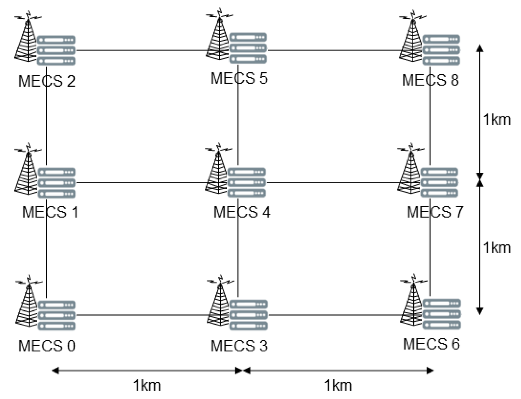
5.1. Simulation Setup

In Figure 4, we show the topology of a MEC system we configured for simulation studies. We evenly deploy $M=9$ MECSs in a $3\times 3$ grid, which ranges from (0, 0) to (2 km, 2 km). We locate each MECS at each grid point. We set the number of services that a MEC system provides to 64 ($K=64$) and the cache size of each MECS to $\eta$.

To configure the popularity of each service in each MECS, we use the MovieLens 25 M dataset $\mathcal{D}$ measured from 1 January 2019 to 21 November 2019 by GroupLens Research [42]. The dataset contains 1,202,602 ratings for 41,440 movies by 10,619 users. Assuming the patterns that the users rate the movies are similar to the patterns that they request for the MEC services, we configure the popularity of each service according to the popularity of movies in the dataset. Specifically, we define the popularity of a movie i in $\mathcal{D}$ as $g_i=n_i/{\sum }_{j\in \mathcal{D}}{n}_j$, where $n_i$ is the number of times that a movie i is rated in the dataset. We sort $g_i$ in a descending order and investigate its distribution. We find that the popularity distribution follows the Pareto principle in that the top $20\%$ popular movies take $84.36\%$ of the total movies. Assuming that the popularity of a service in a MEC system will also follow the Pareto principle, we configure the popularity of a service $k\in \mathcal{K}$ in a MECS m by setting its popularity to that of the set of movies as follows. We denote the set of movies belonging to the top $20\%$ popular movies as $\mathcal{P}$. Without loss of generality, we assume that both the elements in $\mathcal{P}$ and those in $\mathcal{D}-\mathcal{P}$ are sorted in a descending order according to $g_i$. We set $p_m=\lfloor 0.2K\rfloor$ and divide the elements in $\mathcal{P}$ evenly into $p_m$ subsets $P_0,\dots ,P_{p_m-1}$. We also divide the elements in $\mathcal{D}-\mathcal{P}$ evenly into $K-p_m$ subsets $P_{p_m},\dots ,P_{K-1}$. To determine the popularity of each service in each MECS, we randomly assign a service identification number $k\in [0,K-1]$ to each subset $P_0,\dots ,P_{K-1}$ without duplication. Therefore, if a number k is assigned to $P_j$, the popularity of the service k in a MECS m becomes ${\alpha }_{m,k}={\sum }_{i\in P_j}{g}_i$.

We denote the service popularity distribution in a MECS m during a time slot t as ${\mathsf{\Psi }}_m\left(t\right)=\left\{{\alpha }_{m,k}\left(t\right)\right|k\in \mathcal{K}\}$. For each MECS $m\in \mathcal{M}$, we set ${\mathsf{\Psi }}_m\left(0\right)$ by randomly assigning a number $k\in [0,K-1]$ to each subset $P_0,\dots ,P_{K-1}$ without duplication. In other words, we set ${\mathsf{\Psi }}_m\left(0\right)\ne {\mathsf{\Psi }}_n\left(0\right)$ if $m\ne n\in \mathcal{M}$. In the beginning of the simulation, we randomly deploy U = 1000 users in the grid according to the Poisson point process and number them from 0 to 999. As time elapses, ${\mathsf{\Psi }}_m\left(t\right)$ changes because of the mobility of users in the MEC system. We set the mobility pattern of each user by using a real-world dataset. Specifically, we use the Divvy historical trip dataset, which records the trip start day and time, trip end day and time, trip start station, and trip end station [43]. Among the historical trip data, we use the dataset $\mathcal{T}$ containing 767,650 trip history in Chicago during July 2023. We set the x-th record in the dataset as the mobility pattern of the user x $\mathtt{mod}$ U in the MEC system. Therefore, the service popularity distribution in the MEC system changes in time and space.

To configure the service request of each user in the MEC system, we use the records in $\mathcal{D}$. For instance, let us consider the a-th record in $\mathcal{D}$, which says that a movie $b\in P_j$ is rated at time c. If a MECS m is the nearest MECS of a user $u=a$ $\mathtt{mod}$ U and k is assigned to $P_j$ in the MECS m, we set that the user u requests the MECS m for a service k at time c. Since there are average U ratings during six hours in $\mathcal{D}$, we set the duration of a time slot $\tau$ to 6 h so that the average number of service requests by each user in the MEC system is one during a time slot. We set the window size $w_a=12$ for both our method and the LSTM method. By using the datasets $\mathcal{D}$ and $\mathcal{T}$, we measure $\mathsf{\Omega }\left(t\right)=\{{\nu }_1\left(t\right),\dots ,{\nu }_m\left(t\right)\}$ at the end of each time slot. We shuffle all $\mathsf{\Omega }\left(t\right)$s and randomly select 90% of them as a training dataset and use the rest as a validation dataset. We use the last 10% of the total $\mathsf{\Omega }\left(t\right)$s as a test dataset. We summarize the parameters used for the simulation study in

Table 5. Parameters used for the simulation study.

Parameter	Value
M	9
K	64
${\eta }_m$	8, 16
$w_a$	12
Service popularity dataset	MovieLens [42]
User mobility dataset	Divvy trip dataset [43]

.

5.2. Prediction Accuracy

We denote the error involved in predicting the popularity of each service k in a MECS m during a time slot t as ${\delta }_{m,k}\left(t\right)={\nu }_{m,k}\left(t\right)-{\widehat{\nu }}_{m,k}\left(t\right)$ and compare the distribution of ${\delta }_{m,k}\left(t\right)$ for all $k\in \mathcal{K}$ in different MECSs in Figure 5. In this figure, we illustrate the results for four different cases based on the applied methods and MECSs. In each subfigure, the x-axis is the service index $k\in [0,K-1]$ and the y-axis is the prediction error. Thus, for each service k, each subfigure shows the distribution of ${\delta }_{m,k}\left(t\right)$ in a MECS m as a box plot. We observe in the figure that regardless of the true popularity of a service, the 75th percentile of ${\delta }_{m,k}$ obtained by our method is smaller than that resulting from the LSTM method. For example, in MECS 4, the 75th percentile of ${\delta }_{m,k}$ is 0.054 when our method is used, while it is 0.11 when the LSTM method is used. In addition, when the LSTM method is used, there are services whose median ${\delta }_{m,k}$s are much higher than those obtained by our method. For example, the ${\delta }_{m,k}$ of the service k = 33 in MECS 4 obtained by our method is 0.080, while it is 0.90 when the LSTM method is used. We also observe that the interquartile range (IQR), which is the difference between the 75th percentile and the 25th percentile, is smaller when our method is applied compared to when the LSTM method is used. For example, in MECS 4, the average IQR acquired by our method is 0.034, while it is 0.046 when the LSTM method is applied. The results are attributed to the manner that each method predicts the service popularity. When the LSTM method is used, each MECS predicts the popularity of each service within its service range, regardless of the service popularity distributions in the other MECSs. On the contrary, our method predicts the popularity of each service in each MECS at the same time by comprehensively considering the service popularity distributions all over the MECSs. Therefore, our method reduces the amount of error in predicting the popularity of each service in each MECS. We obtain the same results in all the other MECSs.

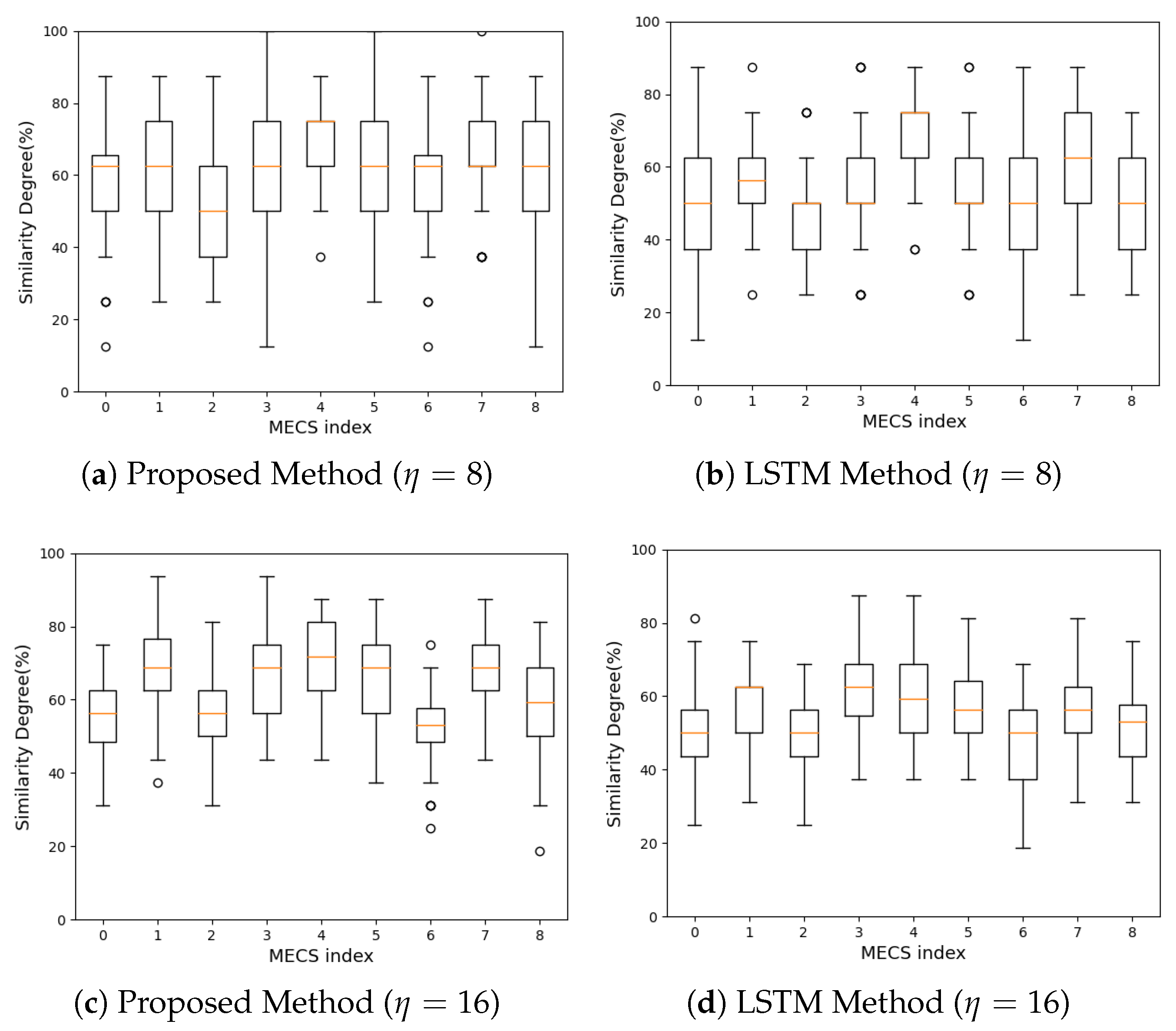
To investigate the influence of the service popularity prediction error on the service caching decision, we inspect the difference between the true $S_m\left(t\right)$ and the predicted $S_m\left(t\right)$ in each MECS m. We note that the true $S_m\left(t\right)$ is composed of the top $\eta$ popular services during a time slot t, which can be known at the end of a time slot t. On the contrary, the predicted $S_m\left(t\right)$ comprises the top $\eta$ popular services whose popularities are estimated by a predictor at the beginning of a time slot t. We denote the true $S_m\left(t\right)$ as $S_m^T\left(t\right)$ and the predicted $S_m\left(t\right)$ as $S_m^P\left(t\right)$. To quantify the similarity between $S_m^T\left(t\right)$ and $S_m^P\left(t\right)$, we calculate $a_m\left(t\right)=|S_m^T\left(t\right)\cap S_m^P\left(t\right)|/\eta$ and show the results in Figure 6 with different $\eta$s. In the figure, we draw the ranges of the y-axis to be the same on purpose to make comparison easier. This figure has four subfigures. In each subfigure, the x-axis is a MECS index m and the y-axis is $a_m$. Each subfigure shows the distribution of $a_m\left(t\right)$ in each MECS as a box plot.

In Figure 6, we observe that our method improves the similarity of the service cache regardless of the MECS position in the grid and the cache size. When $\eta =8$, compared with the LSTM model, our method achieves an $11.26\%$ increase in the cache similarity. Specifically, the average $a_m\left(t\right)$ is $54.71\%$ when the LSTM method is used. The average $a_m\left(t\right)$ increases to $60.87\%$ when our method replaces the LSTM method. The standard deviation of $a_m\left(t\right)$ is $5.99\%$ when our method is used, while it is $5.74\%$ when the LSTM method is used. When $\eta =16$, the proposed method improves the average service cache similarity by $13.52\%$. When the LSTM method is used, the average $a_m\left(t\right)$ is $54.45$%. Our method increases the average $a_m\left(t\right)$ to $61.81\%$. The standard deviation of $a_m\left(t\right)$ is $6.56\%$ when our method is used, and it is $5.09\%$ when the LSTM method is used.

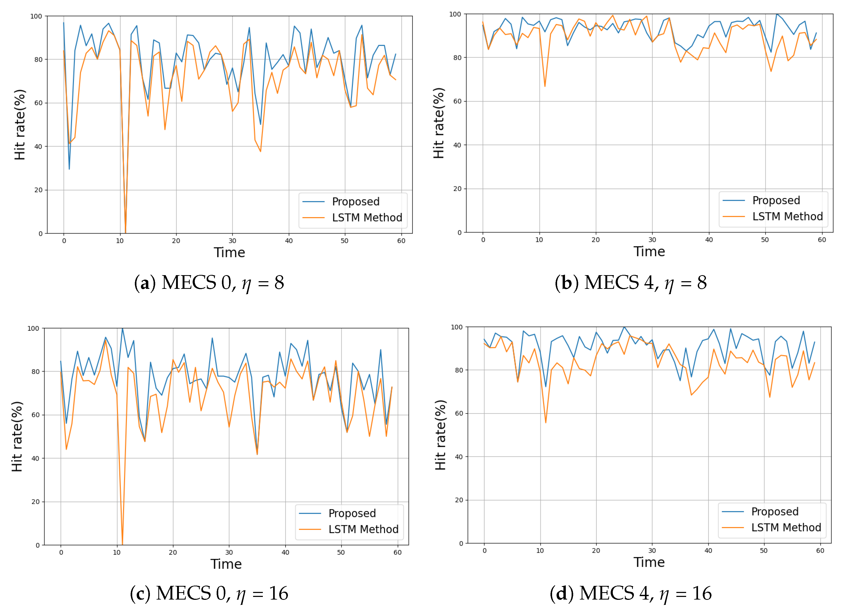
5.3. Hit Rate Comparison

In Figure 7, we show the variations of a cache hit rate in different MECSs with different cache sizes over time. To facilitate the comparison, the ranges of the y-axis in all subfigures are shown to be the same. We observe that the hit rates obtained by our method are higher than those acquired by the LSTM method, regardless of the MECS locations and $\eta$.

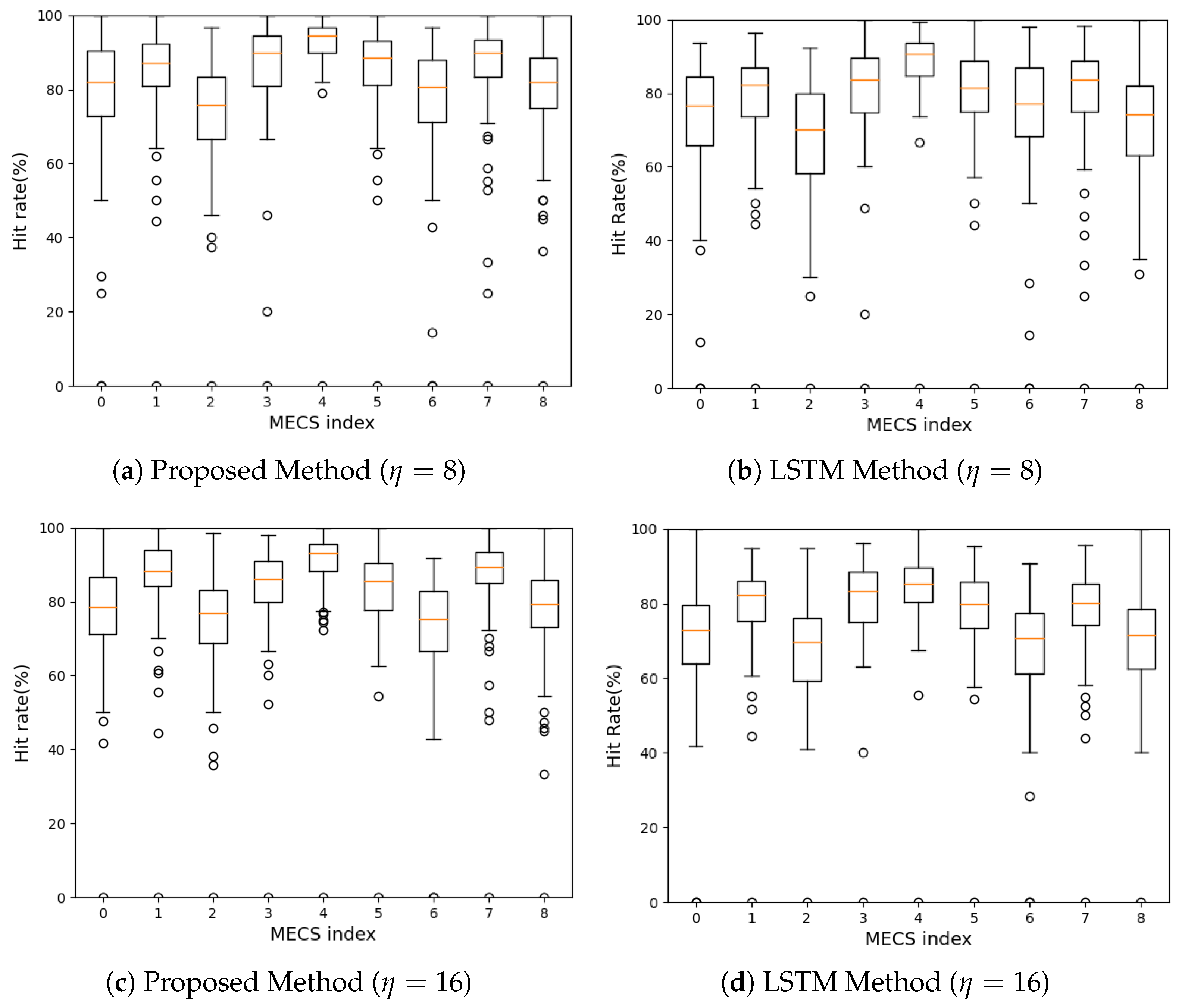
To further verify our method, we compare the distribution of a cache hit rate in each MECS. Specifically, for each MECS, we investigate the difference between the maximum cache hit rate that can be obtained when $S_m^T\left(t\right)$ is used and that acquired when $S_m^P\left(t\right)$ is used. We denote the cache hit rate when $S_m^T\left(t\right)$ is used as $h_m^T\left(t\right)$. We also denote the cache hit rate obtained by a popularity prediction method as $h_m^P\left(t\right)$. For each time slot, we calculate the relative hit rate ${\rho }_m\left(t\right)=h_m^P\left(t\right)/h_m^T\left(t\right)$ and show its distribution in Figure 8. This figure has four subfigures. In each subfigure, the x-axis is a MECS index m and the y-axis is ${\rho }_m\left(t\right)$. Each subfigure shows the distribution of ${\rho }_m\left(t\right)$ in each MECS as a box plot.

In this figure, we observe that the proposed method outperforms the LSTM method in terms of ${\rho }_m$ in all MECSs and $\eta$s. When $\eta =8$, the average ${\rho }_m\left(t\right)$ is 82.13% when our method is used, while it is 76.78% when the LSTM method is used. In other words, our method improves the average cache hit rate by 6.97%. In the case of $\eta =16$, the proposed method enhances the average cache hit rate by 8.48%. The average ${\rho }_m\left(t\right)$ is 81.08% when our method is used, while the average ${\rho }_m\left(t\right)$ obtained by the LSTM method is 74.74%. We also observe that our method decreases the variance in the cache hit rate. When $\eta =8$, the average IQR resulted by the proposed method is 14.19%, while the LSTM method produces an average IQR of 15.88%. In the case of $\eta =16$, the proposed method achieves an average IQR of 11.76%, while it is 13.55% when the LSTM method is used. By decreasing the average IQR by more than 10%, our method makes the cache hit rate in a MEC system stabler than the LSTM method.

We also note that the proposed method needs only one ConvLSTM model to predict the popularity of each service in each MECS. On the contrary, since each MECS needs at least one LSTM model to predict the popularity of each service within only its service area, the LSTM method needs the M LSTM model to predict the service popularity in a MEC system. As we show in Table 4, we use a total of 746,689 parameters for the ConvLSTM model and 121,301 parameters for a single LSTM model. Since the LSTM method uses a total of $M\times \mathrm{121,301}$ model parameters, the proposed method reduces the total model parameters by $32.15\%$. Therefore, when we consider these facts along with the results observed in Figure 8 in an integrated manner, our method can achieve a higher cache hit rate with a smaller amount of model parameters compared to the LSTM method.

5.4. Caching Behavior

We also scrutinize the caching behavior of each method. Instead of predicting the exact order of the service popularity in each MECS, we aim to predict a set of $\eta$ services whose popularity is relatively higher than those of the rest of the services. To quantify the service caching behavior, for each time slot, we calculate $b_m\left(t\right)=|S_m^T\left(t\right)-S_m^T(t+1)|/\eta$ and ${\tilde{b}}_m\left(t\right)=|S_m^P\left(t\right)-S_m^P(t+1)|/\eta$ and plot them in Figure 9 for different m and $\eta$.

We observe that both our method and the LSTM method are conservative in that they do not change the elements in the service cache abruptly. In addition, we observe that the changing pattern of ${\tilde{b}}_m\left(t\right)$ is more similar to that of $b_m\left(t\right)$ when the LSTM method is used compared to when our method is used. This difference in the caching behavior comes from the manner that each method predicts the service popularity. The LSTM method uses only the history of ${\nu }_{m,k}\left(t\right)$ when it predicts ${\widehat{\nu }}_{m,k}(t+1)$ without considering the history of ${\nu }_{n,j}\left(t\right)$s $(n\in \mathcal{M}-\{m\},k\in \mathcal{K}-\{k\left\}\right)$. On the contrary, when our method predicts the service popularity, our method collectively considers not only the temporal correlation but also the spatial correlation. Consequently, compared with the LSTM method, our method responds less sensitively to the instant changes in the service popularity at a single MECS.

5.5. Effect of User Mobility

To inspect the effect of user mobility on the service cache performance, we conducted the same simulation but with a change in the user mobility model from the previous one to a random mobility model, while maintaining the same experimental environment. In a random mobility model, a user changes its moving direction from $(0,{360}^{\circ })$ and speed from $[0,\varsigma ]$ at each time slot according to the Uniform random distribution. Considering the size of the simulation topology, we conduct simulations for the cases where the $\varsigma$ is 0.2 km and 0.5 km.

In Figure 10, we show the distribution of the relative cache hit rate ${\rho }_m\left(t\right)$ with different $\varsigma$ when the cache size is $\eta =8$. In this figure, we observe that the cache hit rate decreases as $\varsigma$ increases. This is attributed to the fact that the increased mobility speed leads to a larger change in the service popularity distribution across each MECS. As a result, the popularity prediction accuracy decreases. In this figure, we also observe that for all the moving speeds, the median ${\rho }_m\left(t\right)$ at all MECS is higher when using the proposed method compared to using the LSTM method. When $\varsigma =0.2$ km, the average cache hit rate rate across all MECS ($\rho \left(t\right)=\frac{1}{M}{\sum }_{i\in \mathcal{M}}{\rho }_m\left(t\right)$) is 85.32% when using the proposed method, while it is 80.88% when using the LSTM method. When $\varsigma =0.5$ km, the average $\rho \left(t\right)$ obtained through the proposed method is 80.92%, while the average $\rho \left(t\right)$ is 74.79% when the LSTM method is used.

5.6. Effect of Service Popularity Variation

To assess the impact of the degree of service popularity change at each MECS on the caching performance, we conduct the following simulations. We extend the topology by deploying $M=16$ MECSs in a $4\times 4$ grid, which ranges from (0,0) to (3 km,3 km). We locate each MECS at each grid point. We also increase the number of services from 64 to 128 and set $\eta$ to 16. For each service k and each MECS m, we randomly change the popularity of a service k at a MECS m at each time slot. To control the degree of service popularity change at each MECS, at the beginning of each time slot, we randomly configure $v_{m,k}(t+1)=v_{m,k}\left(t\right)+x\left(t\right)y\left(t\right)$ ($\forall m\in \mathcal{M},k\in \mathcal{K}$), where $x\left(t\right)$ is determined with a probability of $1/2$ to be either 1 or −1. We randomly select $y\left(t\right)$ from $[0,\xi ]$ according to the Uniform distribution.

In Figure 11, we show the distribution of the cache similarity degree ($a_m\left(t\right)$) with different $\xi$. We oberve that as the degree of service popularity change at each MECS (i.e., $\xi$) increases, the cache similarity degree decreases. In the case of the proposed method, the average $a_m\left(t\right)$ is 98.47% when $\xi =0.05$, while is is 96.19% when $\xi =0.15$. We also observe in this figure that the proposed method outperforms the LSTM method. For all MECSs and $\xi$s, the cache similarity degree is higher when using the proposed method than when using the LSTM method.

6. Conclusions and Future Works

In this paper, we address the service caching problem in a multi-access edge computing system. To increase the cache hit rate, we comprehensively exploit the spatio-temporal correlation structure in the service popularity distribution among the MECSs by using the ConvLSTM model. To achieve the goal, we construct a heatmap to collectively represent the service popularity distribution in a MEC system during a time slot. Using a sequence of heatmaps as an input to the ConvLSTM model, we simultaneously predict the popularity of each service in each MECS. We evaluate the performance of the proposed method through trace-driven simulations. The results verify that compared with a conventional method based on the LSTM model, the proposed method increases the cache hit rate by more than $6.97\%$. In addition, our method reduces the amount of storage required for predicting the popularity of each service in each MECS by $32.15\%$.

Our future works are as follows. Firstly, we will continue our research to further enhance the prediction accuracy. To verify our method, we used the MovieLens dataset and Divvy mobility dataset. We will use other datasets on the user mobility and the service request patterns and show the generality of the proposed method. We will also investigate the explainability of our cache decision algorithm.

References

1. Wang, F.; Cai, S.; Lau, V.K.N. Decentralized DNN Task Partitioning and Offloading Control in MEC Systems With Energy Harvesting Devices. IEEE J. Sel. Top. Signal Process. 2023, 17, 173–188. [Google Scholar] [CrossRef]
2. Siriwardhana, Y.; Porambage, P.; Liyanage, M.; Ylianttila, M. A Survey on Mobile Augmented Reality With 5G Mobile Edge Computing: Architectures, Applications, and Technical Aspects. IEEE Commun. Surv. Tutor. 2021, 23, 1160–1192. [Google Scholar] [CrossRef]
3. Khan, A.u.R.; Othman, M.; Madani, S.A.; Khan, S.U. A Survey of Mobile Cloud Computing Application Models. IEEE Commun. Surv. Tutor. 2013, 16, 393–413. [Google Scholar] [CrossRef]
4. Xu, F.; Liu, F.; Jin, H.; Vasilakos, A.V. Managing Performance Overhead of Virtual Machines in Cloud Computing: A Survey, State of the Art, and Future Directions. Proc. IEEE 2014, 101, 11–31. [Google Scholar] [CrossRef]
5. Ren, D.; Gui, X.; Zhang, K. Adaptive Request Scheduling and Service Caching for MEC-Assisted IoT Networks: An Online Learning Approach. IEEE Internet Things J. 2022, 9, 17372–17386. [Google Scholar] [CrossRef]
6. Liu, H.; Eldarrat, F.; Alqahtani, H.; Reznik, A.; de Foy, X.; Zhang, Y. Mobile Edge Cloud System: Architectures, Challenges, and Approaches. IEEE Syst. J. 2018, 12, 2495–2508. [Google Scholar] [CrossRef]
7. Taleb, T.; Samdanis, K.; Mada, B.; Flinck, H.; Dutta, S.; Sabella, D. On Multi-Access Edge Computing: A Survey of the Emerging 5G Network Edge Cloud Architecture and Orchestration. IEEE Commun. Surv. Tutor. 2017, 19, 1657–1681. [Google Scholar] [CrossRef]
8. Abbas, N.; Zhang, Y.; Taherkordi, A.; Skeie, T. Mobile Edge Computing: A Survey. IEEE Internet Things J. 2018, 5, 450–465. [Google Scholar] [CrossRef]
9. Mach, P.; Becvar, Z. Mobile Edge Computing: A Survey on Architecture and Computation Offloading. IEEE Commun. Surv. Tutor. 2017, 19, 1628–1656. [Google Scholar] [CrossRef]
10. Fan, W.; Yao, L.; Han, J.; Wu, F.; Liu, Y. Game-Based Multitype Task Offloading Among Mobile-Edge-Computing-Enabled Base Stations. IEEE Internet Things J. 2021, 8, 17691–17704. [Google Scholar] [CrossRef]
11. Anajemba, J.H.; Yue, T.; Iwendi, C.; Alenezi, M.; Mittal, M. Optimal Cooperative Offloading Scheme for Energy Efficient Multi-Access Edge Computation. IEEE Access 2020, 8, 53931–53941. [Google Scholar] [CrossRef]
12. Wu, H.; Chen, J.; Nguyen, T.N.; Tang, H. Lyapunov-Guided Delay-Aware Energy Efficient Offloading in IIoT-MEC Systems. IEEE Trans. Ind. Inform. 2023, 19, 2117–2128. [Google Scholar] [CrossRef]
13. Spinelli, F.; Mancuso, V. Toward Enabled Industrial Verticals in 5G: A Survey on MEC-Based Approaches to Provisioning and Flexibility. IEEE Commun. Surv. Tutor. 2021, 23, 596–630. [Google Scholar] [CrossRef]
14. Djigal, H.; Xu, J.; Liu, L.; Zhang, Y. Machine and Deep Learning for Resource Allocation in Multi-Access Edge Computing: A Survey. IEEE Commun. Surv. Tutor. 2022, 24, 2449–2494. [Google Scholar] [CrossRef]
15. Liang, J.; Zhu, D.; Liu, H.; Ping, H.; Li, T.; Zhang, H.; Geng, L.; Liu, Y. Multi-Head Attention Based Popularity Prediction Caching in Social Content-Centric Networking With Mobile Edge Computing. IEEE Commun. Lett. 2021, 25, 508–512. [Google Scholar] [CrossRef]
16. Ale, L.; Zhang, N.; Wu, H.; Chen, D.; Han, T. Online Proactive Caching in Mobile Edge Computing Using Bidirectional Deep Recurrent Neural Network. IEEE Internet Things J. 2019, 6, 5520–5530. [Google Scholar] [CrossRef]
17. Shi, X.; Chen, Z.; Wang, H.; Yeung, D.-Y. Convolutional LSTM Network: A Machine Learning Approach for Precipitation Nowcasting. In Proceedings of the 28th International Conference on Neural Information Processing Systems (NIPS’15), Montreal, QU, Canada, 7–12 December 2015. [Google Scholar]
18. Zhang, H.; Li, X.; Ren, K.; Ren, X.; Penglun, L.; Wang, L. ConvLSTM-CRF: Sea Ice Concentration Prediction with ConvLSTM and Conditional Random Fields. In Proceedings of the 2022 IEEE International Conference on Systems, Man, and Cybernetics (SMC), Prague, Czech Republic, 9–12 October 2022. [Google Scholar]
19. Yan, J.; Bi, S.; Duan, L.; Zhang, Y.-A. Pricing-Driven Service Caching and Task Offloading in Mobile Edge Computing. IEEE Trans. Wirel. Commun. 2021, 20, 4495–4512. [Google Scholar] [CrossRef]
20. Feng, H.; Guo, S.; Liu, D.; Yang, Y. Mean-Field Game Theory Based Optimal Caching Control in Mobile Edge Computing. IEEE Trans. Mob. Comput. 2022, 22, 6585–6598. [Google Scholar] [CrossRef]
21. Liy, N.; Zhuy, X.; Liy, Y.; Wangy, L.; Zhai, L. Service Caching and Task Offloading of Internet of Things Devices Guided by Lyapunov Optimization. In Proceedings of the 2022 IEEE ISPA/BDCloud/SocialCom/SustainCom, Melbourne, VIC, Australia, 17–19 December 2022. [Google Scholar]
22. Bai, Y.; Wang, D.; Song, B. A Knowledge Graph-based Cooperative Caching Scheme in MEC-enabled Heterogeneous Networks. In Proceedings of the 2022 IEEE Global Communications Conference (GLOBECOM), Rio de Janeiro, Brazil, 4–8 December 2022. [Google Scholar]
23. Kirilin, V.; Sundarrajan, A.; Gorinsky, S.; Sitaraman, R.K. RLCache: Learning-Based Cache Admission for Content Delivery. In Proceedings of the 2019 Workshop on Network Meets AI & ML (NetAI’19), Beijing, China, 23 August 2019. [Google Scholar]
24. He, P.; Cao, L.; Cui, Y.; Wang, R.; Wu, D. Multi-Agent Caching Strategy for Spatial-Temporal Popularity in IoV. IEEE Trans. Veh. Technol. 2023, 72, 13536–13546. [Google Scholar] [CrossRef]
25. Narayanan, A.; Verma, S.; Ramadan, E.; Babaie, P.; Zhang, Z.-L. Deepcache: A Deep Learning Based Framework for Content Caching. In Proceedings of the 2018 Workshop on Network Meets AI & ML (NetAI’18), Budapest, Hungary, 24 August 2018. [Google Scholar]
26. Lekharu, A.; Jain, M.; Sur, A.; Sarkar, A. Deep Learning Model for Content Aware Caching at MEC Servers. IEee Trans. Netw. Serv. Manag. 2022, 19, 1413–1425. [Google Scholar] [CrossRef]
27. Kang, M.W.; Chung, Y.W. Content Caching Based on Popularity and Priority of Content Using seq2seq LSTM in ICN. IEEE Access 2023, 11, 16831–16842. [Google Scholar] [CrossRef]
28. Meybodi, Z.H.; Mohammadi, A.; Rahimian, E.; Heidarian, S.; Abouei, J.; Plataniotis, K.N. TEDGE-Caching: Transformer-based Edge Caching Towards 6G Networks. In Proceedings of the IEEE International Conference on Communications (ICC 2022), Seoul, Republic of Korea, 16–20 May 2022. [Google Scholar]
29. Meybodi, Z.H.; Mohammadi, A.; Abouei, J.; Plataniotis, K.N. CoPo: Self-supervised Contrastive Learning for Popularity Prediction in MEC Networks. In Proceedings of the 2023 IEEE 24th International Conference on Digital Signal Processing (DSP), Rhodes, Greece, 11–13 June 2023. [Google Scholar]
30. HajiAkhondi-Meybodi, Z.; Mohammadi, A.; Hou, M.; Abouei, J.; Plataniotis, K.N. ViT-Cat: Parallel Vision Transformers With Cross Attention Fusion for Popularity Prediction in MEC Networks. In Proceedings of the 2023 IEEE International Conference on Acoustics, Speech and Signal Processing (ICASSP), Rhodes Island, Greece, 4–10 June 2023. [Google Scholar]
31. Wang, K.; Deng, N.; Li, X. An Efficient Content Popularity Prediction of Privacy Preserving Based on Federated Learning and Wasserstein GAN. IEEE Internet Things J. 2022, 10, 3786–3798. [Google Scholar] [CrossRef]
32. Xiao, K.; Zhao, J.; He, Y.; Yu, S. Trajectory Prediction of UAV in Smart City using Recurrent Neural Networks. In Proceedings of the 2019 IEEE International Conference on Communications (ICC), Shanghai, China, 20–24 May 2019. [Google Scholar]
33. Sahoo, B.B.; Jha, R.; Singh, A.; Kumar, D. Long Short-Term Memory (LSTM) Recurrent Neural Network for Low-Flow Hydrological Time Series Forecasting. Springer Acta Geophys. 2019, 67, 1471–1481. [Google Scholar] [CrossRef]
34. Liu, Y.; Wang, Z.; Zheng, B. Application of Regularized GRU-LSTM Model in Stock Price Prediction. In Proceedings of the 2019 IEEE 5th International Conference on Computer and Communications (ICCC), Chengdu, China, 6–9 December 2019. [Google Scholar]
35. Shih, S.-Y.; Sun, F.-K.; Lee, H.-y. Temporal Pattern Attention for Multivariate Time Series Forecasting. Springer Mach. Learn. 2019, 108, 1421–1441. [Google Scholar] [CrossRef]
36. Fan, C.; Zhang, Y.; Pan, Y.; Li, X.; Zhang, C.; Yuan, R.; Wu, D.; Wang, W.; Pei, J.; Huang, H. Multi-Horizon Time Series Forecasting with Temporal Attention Learning. In Proceedings of the 25th ACM SIGKDD International Conference on Knowledge Discovery & Data Mining (KDD ’19), Anchorage, AK, USA, 4–8 August 2019. [Google Scholar]
37. Oreshkin, B.N.; Carpov, D.; Chapados, N.; Bengio, Y. N-BEATS: Neural Basis Expansion Analysis for Interpretable Time Series Forecasting. In Proceedings of the eighth International Conference on Learning Representations, Virtual Conference, 26 April–1 May 2020. [Google Scholar]
38. Challu, C.; Olivares, K.G.; Oreshkin, B.N.; Garza, F.; Mergenthaler-Canseco, M.; Dubrawski, A. N-HiTS: Neural Hierarchical Interpolation for Time Series Forecasting. In Proceedings of the Thirty-Seventh AAAI Conference on Artificial Intelligence, Washington, DC, USA, 7–14 February 2023. [Google Scholar]
39. Zhou, Y.; Dong, H.; Saddik, A.E. Deep Learning in Next-Frame Prediction: A Benchmark Review. IEEE Access 2020, 8, 69273–69283. [Google Scholar] [CrossRef]
40. Joshi, A. Next-Frame Video Prediction with Convolutional LSTMs. Available online: https://keras.io/examples/vision/conv_lstm (accessed on 5 June 2021).
41. Brownlee, J. A Gentle Introduction to LSTM Autoencoders. Available online: https://machinelearningmastery.com/lstm-autoencoders (accessed on 27 August 2020).
42. Harper, F.M.; Konstan, J.A. The Movielens Datasets: History and Context. ACM Trans. Interact. Intell. Syst. 2015, 5, 1–19. Available online: https://grouplens.org/datasets/movielens (accessed on 1 January 2019). [CrossRef]
43. Divvy Historical Trip Data. Available online: https://divvybikes.com/system-data (accessed on 14 August 2023).
Figure 1. The inner structure of a ConvLSTM cell at time step t. The operator ∗ represents the convolutional operation, and ∘ denotes the Hardmard product. In addition, σ represents the sigmoid function, and tanh represents the hyperbolic tangent function.
Applsci 13 12509 g001
Figure 2. System model.
Applsci 13 12509 g002
Figure 3. Service cache decision procedure.
Applsci 13 12509 g003
Figure 4. Topology of a MEC system.
Applsci 13 12509 g004
Figure 5. Distribution of the prediction error for each service k K in different MECSs. MECS 4 is located at the center of the grid, and MECS 0 is located at the bottom left corner of the grid. Each subfigure shows the distribution of δ m , k ( t ) in each MECS as a box plot.
Applsci 13 12509 g005aApplsci 13 12509 g005b
Figure 6. Service cache similarity at each MECS with different η s. Each subfigure shows the distribution of the service cache similarity in each MECS as a box plot.
Applsci 13 12509 g006
Figure 7. Comparison of a cache hit rate over time in different MECSs.
Applsci 13 12509 g007
Figure 8. Comparison of the distribution of the relative cache hit rate in each MECS. Each subfigure shows the distribution of ρ m ( t ) in each MECS as a box plot.
Applsci 13 12509 g008
Figure 9. Comparison of caching behavior.
Applsci 13 12509 g009
Figure 10. Distribution of the relative cache hit rate at each MECS when a cache size is η = 8 .
Applsci 13 12509 g010
Figure 11. Distribution of the cache similarity degree when η = 16 , K = 128 , and M = 16 .
Applsci 13 12509 g011