Harnessing Energy Balance and Genetic Algorithms for Efficient Building Demolition

Abstract

In the realm of building demolition, ensuring the uniform distribution of energy from multiple sources is of paramount significance for the systematic deconstruction of large structures. This study presents an integrated methodology that combines genetic optimization and potential energy balance to determine the most suitable locations for multiple energy release points, thereby enhancing the efficiency and reliability of the demolition process. We initiate our approach by randomly selecting energy release points within a building model and subsequently simulate energy dispersion utilizing a potential function until reaching stable boundaries. In instances where the discrepancy in the area between the regions with maximum and minimum energy dispersion exceeds a predefined threshold, we instigate an optimization process employing genetic algorithms. This optimization process involves genetic crossover and mutation operations, followed by subsequent energy balance calculations. The result is not only an improvement in demolition efficiency but also an assurance of even energy coverage throughout the target area.

1. Introduction

The debate surrounding whether aging buildings should be renovated or demolished to make way for new construction has been long-standing and intense. Research indicates that, influenced by factors such as investment costs and the future market value of the building, demolition and new construction may be the more advantageous choice in certain circumstances [1]. In the field of modern architecture, when faced with the task of demolishing large structures, obtaining useful data and guiding information about building demolition can aid in achieving more efficient and safe demolition work [2]. Among this useful information, the precise positioning of energy release points is crucial. This precision is vital not only to ensure that each energy release point fully covers the target area but also to prevent overlap, which could reduce the efficiency of the demolition process. Modern building demolition often requires operating multiple energy release points simultaneously on large structures; thus, the focus has shifted to how to achieve precise energy coverage and methods for reducing overlap when multiple energy release points are involved. In the demolition process, how to conserve resources consumed in demolition is key to making the end-of-life stage of buildings more sustainable [3].

Michaloudis G proposed that when buildings are no longer in use, they need to be demolished in a controlled manner, and the use of controlled explosives is a highly efficient method. To ensure the safety of surrounding buildings and traffic, it is necessary to reliably predict the specific collapse dynamics caused by the explosion, which requires a reliable simulation of the entire collapse process [4]. Pourasil and others discussed the demolition methods at the end of a building’s life cycle, especially the use of controlled blasting, emphasizing the importance of mixed demolition methods, including controlled blasting, for achieving the sustainability and resource recovery of construction projects [5]. Zahedi, M.’s research provides a reliable method of controlled blasting construction by systematically selecting the columns to be demolished. The results show that better blasting effects can be achieved in multi-stage blasting plans by removing columns that contribute more to key structural elements, especially in lower structural parts [6]. Although this research has achieved better demolition effects, it only targets the internal structure of the building and does not consider how to demolish under multi-point energy release. Ibrahim and others developed a detailed 3-D finite element model using the Abaques 2020 software package to study the response of an existing six-story reinforced concrete frame structure in Saudi Arabia under explosive loads. The research also considered the use of external columns with a composite section design of steel shells surrounding concrete sections, which achieved better results in mitigating the effects of explosive loads [7]. This research still focuses more on the internal structure of the building and only targets one building, without discussing various types of buildings. Jayasooriya, R. used dynamic computer simulation technology to explore the response, damage mechanism, and residual bearing capacity of concrete–steel composite (CSC) columns under explosion. The results show that compared with reinforced concrete (RC) columns of the same size and steel ratio, CSC columns perform well in terms of residual bearing capacity and have the potential to become key elements in a structural system [8]. Zhou, X. studied the blasting demolition of high-rise steel structure buildings through a computer video image simulation and used the LS-DYNA R13.0 software updated with the core algorithm for a specific blasting demolition work simulation. The experimental results show that the updated algorithm improves the accuracy of the simulation results, with a similarity of up to 97% with the actual demolition work, and the risk comparison probability also increased by nearly 31% [9]. However, this research only improves the simulation software algorithm and does not provide guidance for actual demolition work.

Although the aforementioned research proposes some simulation methods for building demolition, it is more concerned with the internal structure of the building and does not categorize the shape of the demolished building into multiple categories. Instead, it discusses single-structure buildings more often, which limits the generalizability of the research results in real life. In reality, it is more common for multiple energy release points to act on different buildings. This requires not only that multiple energy release points achieve boundary energy balance but also that attention be paid to the uniformity of the energy diffusion area. When demolishing a building, the diffusion function (potential function) of the energy release point often adopts the point release shock wave overpressure formula, which can better express the diffusion situation when each source point releases energy, and has practical significance [10].

After determining the calculation of multi-source point energy diffusion, we need to consider how to make the diffusion area as uniform as possible, which is essentially an optimization problem. The core of the optimization problem is to find the maximum or minimum value of the objective function under given constraints. This usually involves determining the optimal value of one or more variables to make the objective function reach its optimal (maximum or minimum) value, while satisfying all constraints. Common optimization strategies include genetic algorithms [11], simulated annealing algorithms [12], etc. The scholar Yong, Z. proposed a new multi-objective evolutionary method for optimizing the energy performance of buildings in China, with the main goal of minimizing energy consumption and maximizing comfort. The paper introduces an improved bare-bones particle swarm optimization algorithm, which outperforms other comparative algorithms in obtaining good non-dominated solutions, reducing the number of uncomfortable hours by 11.82%, while energy consumption only increased by 1.74%, making it a powerful tool for optimizing building energy performance. This research is aimed at energy consumption and does not consider the field of building demolition [13]. In addition, scholars have optimized the layout of building structures to meet environmental performance standards based on the simulated annealing algorithm [14]. In terms of genetic algorithms, many scholars have carried out the multi-objective optimization of building design based on genetic algorithms [15], and some research has improved this, using genetic algorithms and artificial neural networks for the multi-objective optimization of building design [16]. Some scholars have also proposed a method for generating the layout of modular high-rise residential buildings (MHRB) based on genetic algorithms [17]. Turrin used parametric modeling and genetic algorithms to design buildings, taking the example of solar energy transmission to the roof. This research involves fewer types of buildings and does not consider the process and results of multiple energy actions [18]. Luo, X. proposed an adaptive deep neural network for building energy consumption prediction based on reaction and genetic algorithms [19]. In addition to the field of building resource allocation, optimization strategies also play many roles in energy release. Tsuga, T, combined multi-objective genetic algorithms (MOGAs), surrogate models, and Kriging techniques to evaluate the worst-case scenario of explosive destruction. However, this research still only considers the worst-case scenario and does not discuss multiple scenarios [20]. Babanouri used a simulated annealing search algorithm to estimate the coupled method of unknown characteristics when studying the propagation of explosion waves in fractured rock masses [21].

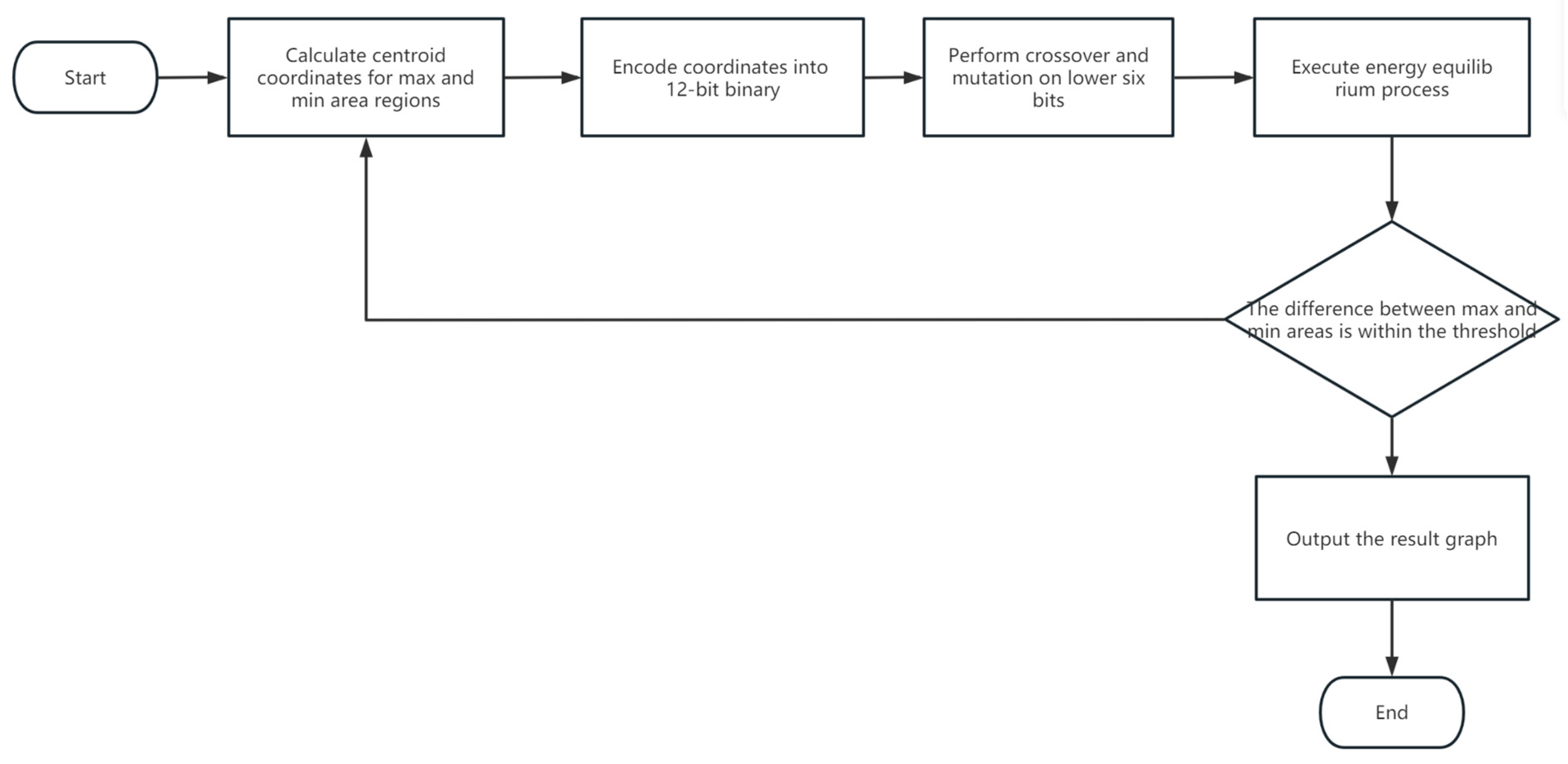
Although the aforementioned research involves building demolition and energy release, it only considers the internal structure of the building, neglecting the energy release on the surface, and it does not take into account the diversity of building structures. Moreover, it does not consider the process and results of multi-point energy release. In optimization strategies, genetic algorithms and simulated annealing algorithms are more often used to study house energy distributions and house structure layouts and have not been combined with building demolition and multi-point energy release on the building surface. In order to achieve a balance at the boundary during energy release from multiple energy release points and to make the area of each energy release coverage area as uniform as possible, this study presents an optimization strategy that combines genetic algorithms with a potential function to achieve an energy equilibrium. Initially, each release point is viewed as a source of energy diffusion. The energy spread is then modeled using a potential function until the boundary energy of each diffusion area stabilizes. Subsequently, the center of the diffusion range is used as a new reference point for further energy diffusion calculations. This iterative process continues until the difference between two consecutive calculations is within a predefined error margin, ensuring a balanced energy distribution. If the difference between the largest and smallest diffusion areas surpasses a set threshold, a secondary optimization using the genetic algorithm is triggered. During this phase, the effective energy coverage area for each release is identified, and its center coordinates (i.e., release points) are encoded into a 12-bit binary format. By selecting the encodings corresponding to the largest and smallest energy coverage areas, two random bits from the lower six bits are subjected to crossover and mutation operations. The resulting new encoding then becomes the new release point for the next round of energy balance calculations. This optimization cycle repeats until the difference between the largest and smallest energy coverage areas meets the acceptable error range.

The primary contributions of this study can be summarized in the following areas: First, we propose a unique optimization strategy that addresses the challenges of overlapping coverage and uneven energy distribution at diffusion points, leading to improved precision and efficiency in energy dissemination. Second, by merging an enhanced genetic algorithm with potential function energy equalization, our research presents a practical method for refining energy dissemination strategies. Finally, through empirical testing, we demonstrate that our proposed optimization approach performs well in terms of the precision and effectiveness of energy dissemination across diverse architectural structures and initial diffusion point placements, providing a valuable perspective in the technical domain.

The organization of this paper is as follows: Section 2 thoroughly introduces our dataset, research methodology, and the algorithms employed, accompanied by mathematical models and an analysis of algorithmic complexity. Section 3 exhibits the experimental outcomes, encompassing iterative graphs and the computational results of numerous experiments. Lastly, Section 4 encapsulates the research and underscores potential avenues for future exploration.

2. Materials and Methods

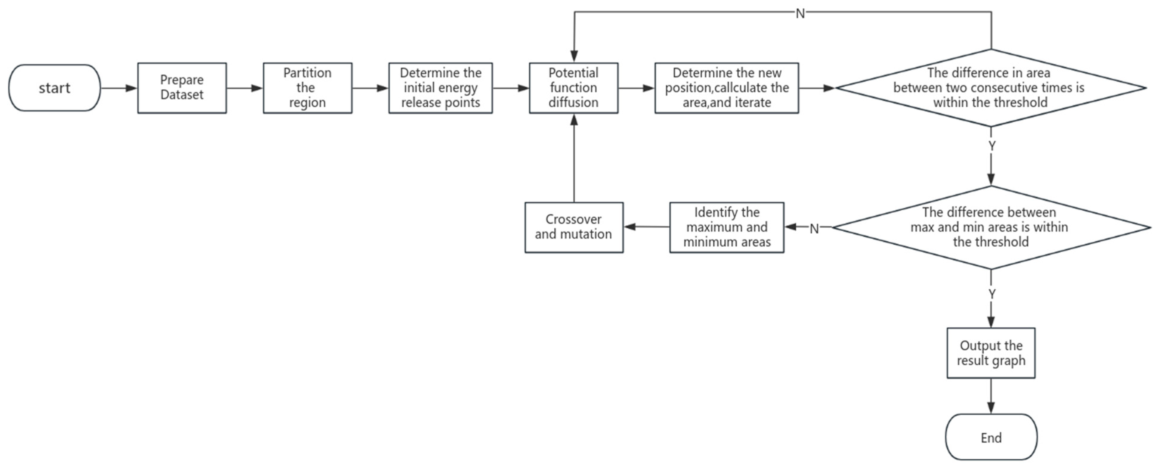
In this section, we offer an in-depth explanation of our method for pinpointing energy dissemination points by merging genetic optimization with potential function energy balancing. Initially, given the distinct features of various buildings, we generated multiple datasets that cover a range of potential energy dissemination scenarios and target characteristics. When identifying energy dissemination points, we utilized an iterative calculation method centered on multi-source energy balancing. Specifically, each dissemination point is viewed as a source of energy diffusion, and its energy spread is modeled using a potential function until the boundary energy of each diffusion area reaches equilibrium. This approach greatly enhances computational speed and swiftly ensures a uniform distribution of energy throughout the designated area.

In practical scenarios, we noted that for some datasets, after multi-source energy diffusion, a significant disparity arises between the largest and smallest coverage areas. To address the challenges of energy dispersion from multiple source points, we employed an optimized genetic algorithm. Initially, after the aforementioned algorithm concludes, we can obtain the area of all current regions, identifying the largest and smallest area. Subsequently, we conduct crossover and mutation operations on the coordinates (genes) of the centers of these maximum and minimum areas, generating new coordinates. We then execute the energy balancing algorithm operations on these new coordinates once again. We consistently iterate the entire procedure until the difference between the maximum and minimum values of the current energy dissemination range meets an acceptable threshold, ensuring all boundaries comply with energy balance standards. Through empirical testing on various datasets, we have validated the effectiveness and versatility of this approach, achieving significant performance improvements. The brief overview of our algorithmic process is as shown in Figure 1.

2.1. Dataset Preparation and Division

In our research, we utilized custom-developed three-dimensional simulation software to construct a series of 3D architectural models, each representing various building types in the real world. To facilitate the simulation process, we selected the top-down views of buildings as input data. Notably, although we displayed the 3D architectural models and their corresponding top-down views, this was solely to illustrate the close relationship between our models and actual buildings. The actual dataset does not include the 3D models.

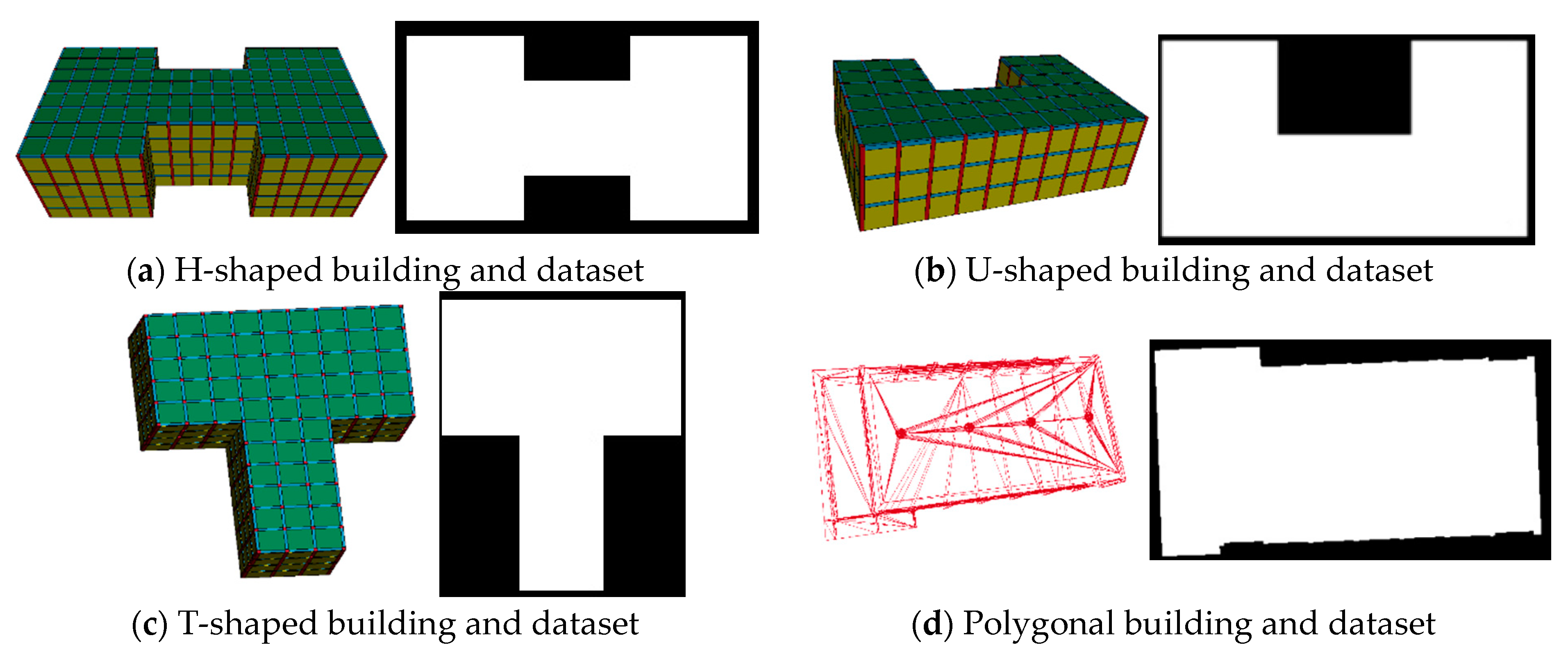
Within our software, we have multiple grids, and we delineate these grid boundaries based on the required data shapes. By specifying the number and size of pixels within the software, it can generate the corresponding experimental input data. In the experimental phase of Section 3, we will provide the dimensions for each set of input data. You can use other image processing software to generate corresponding data based on the provided dimensions and shapes to replicate our results. In actual calculations, the software is used to generate pixel points, which we then represent with a two-dimensional array for the pixel coordinates. After the iterative process, we render the pixels represented by the two-dimensional array and visualize them. Alternatively, you can directly use the two-dimensional array to represent pixel positions and execute the iterative process of our algorithm. Our software is specifically designed to facilitate the visualization process and results. We assure you that our meticulously designed software, created for the convenient generation of input data, employs existing public technologies and will not influence the results in any way. To guarantee the dataset’s diversity and universality, we undertook a comprehensive classification of building forms. In order to enhance our relevance, we selected four different common building types in life; in real life, there are many types of buildings, and the top view of the H, U, T, and polygonal building types tends to be more common. By analyzing data on them, the effect tends to be close to the actual situation and more satisfactory. We categorized the dataset into four major groups—T-shaped, U-shaped, H-shaped, and polygonal—based on the characteristics of the buildings’ top views. These categories not only encompass a wide variety of conventional building structures but also hold practical significance.

To more accurately represent the diversity of energy release point locations, we devised two dataset division strategies for each building form: equal division and random division. Assuming there are n energy release points, the dataset for each building form is divided into n subsets. Under the equal division strategy, the dataset is segmented into n subsets at equal intervals to ensure each subset is balanced in terms of the area and characteristics. Conversely, the random division strategy involves a random segmentation of the dataset, a process that mirrors the uncertainty and complexity encountered in real-world scenarios. The specific building models and datasets are illustrated in Figure 2 as shown.

In summary, this study, through the precise classification of architectural models and meticulous dataset division strategies, lays a robust and diverse data foundation for optimizing energy release points. The aforementioned rigorous classification and division enable our dataset not only to simulate various architectural forms but also to model the initial locations of multiple energy release points accurately. This alignment with actual conditions significantly enhances the accuracy and reliability of the model.

2.2. Multi-Source Energy Balance

The multi-source energy balance is a method designed to ensure that, within a designated area, multiple iterations of energy diffusion and relocation lead to an equilibrium in the energy boundaries of each source point. The core of this method is to determine the optimal influence range for each energy release point through meticulous energy distribution and adjustments. Initially, energy release points are established. Whether these points are located within or outside the target range, they can be fine-tuned to their optimal positions using iterative algorithms. The specific steps for implementing the multi-source energy balance are detailed below:

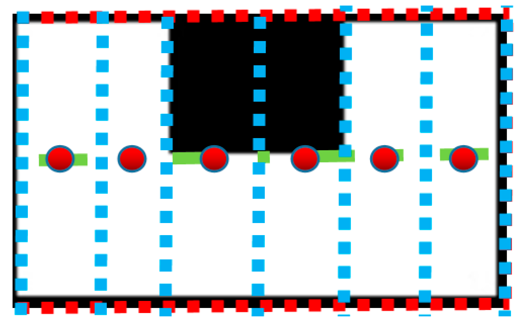
Step 1. The initial step is to determine the energy release points. We first expand our dataset to cover a rectangular area. Using an equal division strategy, we select the midpoint on the median line within each divided area as the initial energy release points. It is important to note that these initial points may be located within or outside the target range. However, through our iterative algorithm, these points can be adjusted to their ideal energy release locations. This method provides an effective way to determine the initial energy release points, laying the groundwork for subsequent optimization processes. For instance, the schematic diagram of equal division for a U-shaped dataset is as shown in Figure 3. The blue, red, and green lines represent the strategies for dividing areas, and the red circles represent the chosen initial positions.

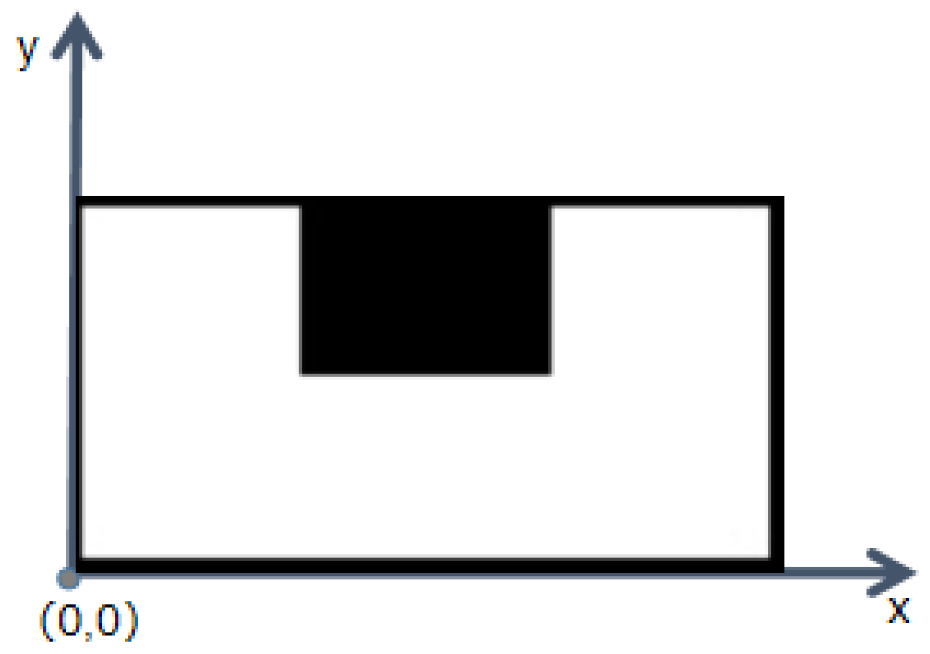
Step 2. In our methodology, we constructed a Cartesian coordinate system based on the dimensions of the rectangular region, designating its vertex as the origin, with both x and y axes scaled in meters. As depicted in Figure 4, using the U-shaped data as a representative example, our dataset encompasses numerous pixel points, which were predefined during the dataset formulation. All subsequent computations are anchored in this coordinate framework. The data are delineated by pixels, with each pixel equating to a physical span of 0.25 m in real-world dimensions. This coordinate system facilitates a meaningful connection between our model and actual architectural structures, thereby bolstering its practical relevance.

Furthermore, for each energy release point within the region, we employ a potential function to model energy diffusion. In our study, the energy transfer process from energy release points constitutes a vital component. To accurately depict this process, we have chosen to utilize the fundamental calculation formula for shock wave overpressure resulting from point energy release. This formula is widely acknowledged as an effective tool for universally characterizing the phenomenon of shock wave overpressure, particularly when energy release points are involved [10]. The formula’s precise depiction of the energy transfer process allows us to delve deeply into the dynamic behavior. The potential function is defined as follows:

$$\mathrm{P}=\frac{0.082}{R}+\frac{0.0265}{R^2}+\frac{0.686}{R^3}$$

(1)

where R represents the proportional distance:

$$\mathrm{R}=\frac{r}{W^{\frac{1}{3}}}$$

(2)

In this context, $r$ represents the distance from the current position to the energy release center (m), while $W$ is the equivalent value of the release amount (kg). The unit of the potential function is given in Mpa.

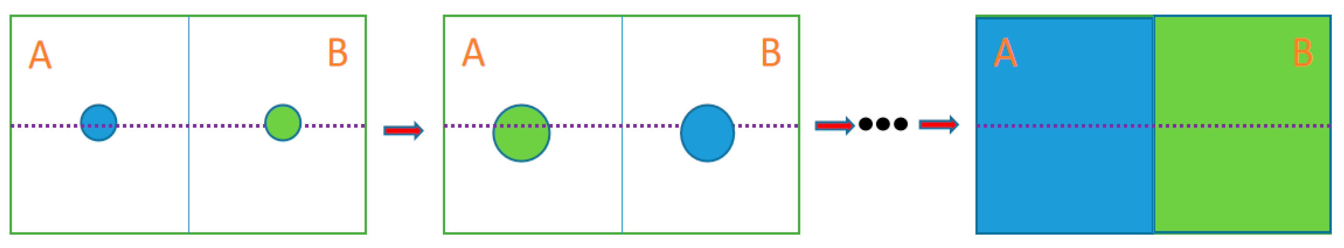
In our algorithm, the initial value of R is set to 0.25 m and is increased by 0.25 m with each iteration. As illustrated in Figure 5, during the first iteration, we first compute the energy diffusion value for Region A, followed by that for Region B. In the subsequent iteration, we reverse the order, starting with Region B and then moving to Region A. Throughout the iterations, we first compute the area where the blue circle is located, followed by the area of the green circle. The iterative calculation will continue until an energy equilibrium is achieved between adjacent boundaries. In each iteration, the initial coordinate values of the energy release points are set to K (where k = 1, 2, …, N), with N denoting the number of energy release points. The values of pixel coordinates passed during the diffusion process are modified to the corresponding K based on the coordinate values of the energy release points. By assessing whether these traversed pixel coordinate values have been preemptively changed, we can ascertain if we have reached the boundary of the adjacent region. In other words, this signifies whether the current iteration has realized the energy balance between adjacent boundaries.

Step 3. After reaching an equilibrium between adjacent boundary regions, we scan through all pixel values. Depending on the distinct K values, we tally the pixels within different regions. With each pixel representing an area of 0.25 m × 0.25 m, we can compute the total area of all regions. Assuming the current region is labeled as $i$, its diffusion area is denoted as $S_i$. We then take the centroid of this diffusion range as the new energy release point and commence the next round of iterative processing.

Steps 2 and 3 are executed repeatedly. The iteration concludes once the condition defined by Equation (3) is satisfied, signaling that the final equilibrium state has been attained. Additionally, $P_1$ represents the error ratio of the difference in area between two iterations. This ratio will be provided in the subsequent experimental setup.

$$\frac{S_c-S_l}{S_l}\le P_1$$

(3)

In Equation (3), $S_c$ represents the area of the region calculated in the current iteration, while $S_l$ represents the area of the region calculated in the previous iteration. When the difference between the two is within $P_1$, we consider that the iteration has reached equilibrium.

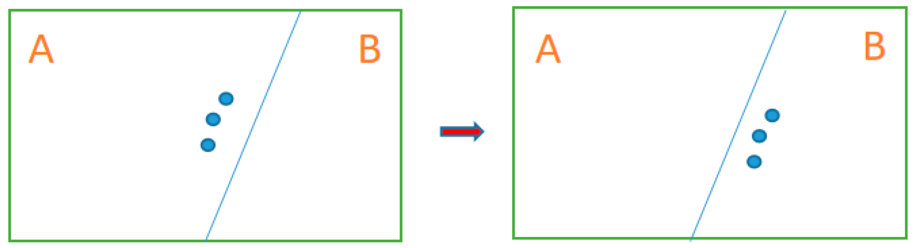
Step 4. Upon the completion of the iterations, we observed a phenomenon termed the “oscillation effect”. According to the potential function formula, pixel oscillations occur at the boundary between two adjacent areas. For instance, as shown in Figure 6, during the initial computation, the energy diffusion value for Area A is calculated first, followed by that for Area B. Consequently, the boundary pixels(blue circles) are attributed to Area A. In the subsequent computation, the order is reversed, with Area B being computed before Area A, resulting in the boundary pixels(blue circles) being attributed to Area B. This variation in pixel attribution due to the change in the computation sequence is what we define as the “oscillation effect”. We further designate the region experiencing this oscillation as the “oscillatory region”. The schematic diagram is as follows:

In each computational process, we consistently record the pixel coordinates of the boundary and keep a record of the traversed pixel blocks, each measuring 0.25 m by 0.25 m. This information is utilized to calculate the diffusion area of the energy release point. Given that the pixels within the “oscillation region” align with the recorded boundary coordinates, we choose to dynamically allocate these oscillating pixel blocks to the region currently being computed, based on the direction of the calculation process. For example, as illustrated in Figure 5, when the boundary oscillation condition is met, and the computation has progressed to the blue-shaded Area A, we assign this oscillation region to Area A. As our algorithm undergoes multiple iterations, each with a very small area error threshold, dynamic allocation continues to yield satisfactory results.

This multi-source point energy balancing method takes into account the even distribution of energy and can achieve the convergence of energy diffusion from multiple sources in a relatively short time. However, after multiple iterations, a small portion of datasets still exhibit significant disparities in the diffusion area of different sources, not meeting the criteria set by the following equation:

$$\frac{S_{max}-S_{min}}{S_{min}}\le P_2$$

(4)

Here, $S_{max}$ represents the maximum area extent, while $S_{min}$ denotes the minimum area extent. $P_2$ signifies the ratio of the difference between the maximum and minimum areas. This ratio will be specified in forthcoming experimental configurations. When the difference between them is within $P_2$, we consider the areas to be essentially balanced.

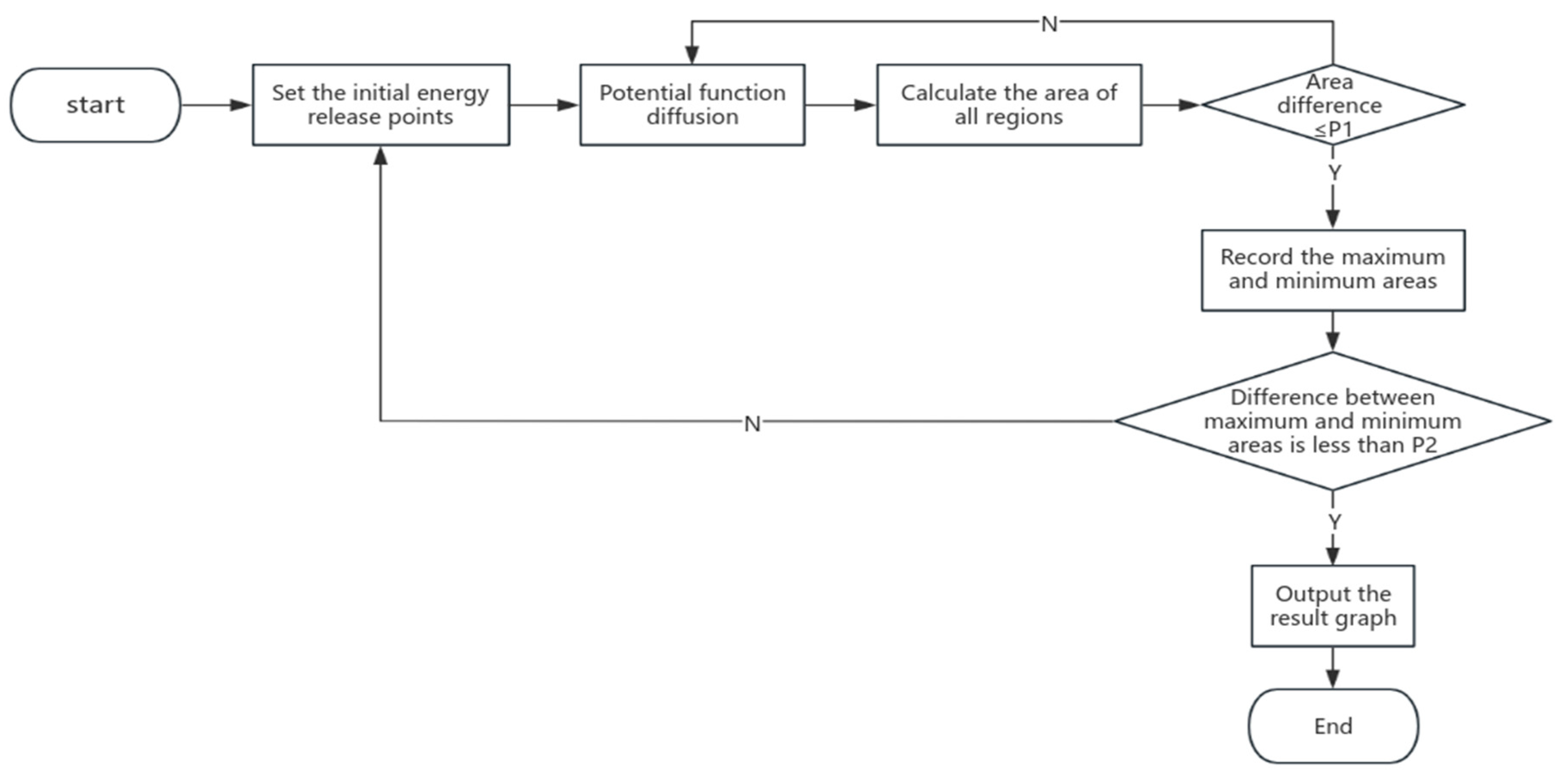
Consequently, we introduced an improved genetic algorithm for optimization. This ensures that while maintaining energy balance, the area differences between regions are minimized, guaranteeing the accuracy of the results. The flowchart of our algorithm for this part is as shown in Figure 7:

2.3. Optimization with an Enhanced Genetic Algorithm

The Genetic Algorithm is an optimization algorithm grounded in Darwin’s Theory of Evolution that is especially apt for tackling complex optimization problems. This algorithm exhibits significant self-learning, self-adaptation, and self-optimization characteristics, as validated in the studies by Meng, X., Bradley, J., Yavuz, B., and others [22]. The fundamental principle of the Genetic Algorithm is encoding each potential solution as a “chromosome,” with each chromosome representing a specific solution. Subsequently, each chromosome is evaluated based on predetermined criteria and ranked according to its fitness. Chromosomes with a higher fitness are more likely to be selected to generate the next generation. Through operations like selection, crossover, and mutation, a new population is generated and used for the next round of evaluation and selection. This process continues until the fitness of a chromosome meets the preset requirements, at which point the solution represented by this chromosome is deemed optimal.

Building on the framework of the traditional Genetic Algorithm, we have made specific algorithmic improvements for the optimization problem of energy release points. In our proposed improved algorithm, genes are represented using binary encoding—specifically, each gene represents a regional center, i.e., the coordinates of the energy release point. To achieve precise localization, we assigned 12-bit binary encoding to each coordinate, with each bit representing 0 or 1, thereby representing 4095 different positions. In this encoding scheme, each pixel value corresponds to an actual distance of 0.25 m; thus, the 12-bit binary encoding represents a physical distance range of 1000 m. A straight-line distance of 1000 m is substantial, encompassing the scale of most architectural structures one might encounter in real-world scenarios. Therefore, this setting is not just about precision; it significantly enhances the algorithm’s applicability and relevance to real-world architectural scenarios.

To ensure that both large and small areas are as close in size as possible, we have devised a specific crossover strategy. After numerous iterations of energy balance adjustments, the positions of the energy release points within each area have been essentially determined, negating the need for major modifications. Consequently, we selected the regions with the largest and smallest coverage areas and executed a crossover operation on the lower six bits of their central coordinate’s binary encoding (gene). The physical distance represented by these six bits is 16 m, a level of precision that is adequate for fine-tuning requirements. Through this crossover operation, we can identify more accurate positions for energy release.

Our algorithm retains the foundational structure of genetic algorithms. By employing innovative encoding schemes and crossover strategies, we have pinpointed more accurate coordinates for the energy release source points. The specific steps are as follows:

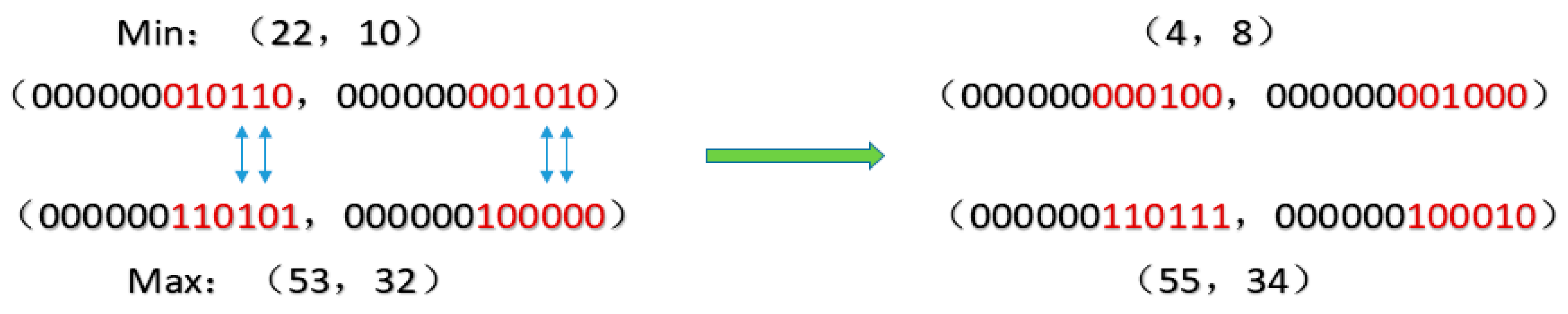
Step 1. Crossover Operation: After several rounds of energy balance adjustments, we have determined the coordinates of energy diffusion source points for each region, as well as the coordinates of the surrounding boundary pixels. Furthermore, we have calculated the area size associated with each source point. We then select the regions with the largest and smallest coverage areas for gene crossover operations, producing new coordinates for energy release source points. This operation specifically alters only two random bits within the lower six bits, with a crossover probability of 0.96. This means there is a 96% likelihood of executing random two-bit crossovers in each iteration. The objective of this operation is to introduce slight modifications while preserving the overall region, aiming for enhanced precision in optimization. For instance, in a specific iteration, if the coordinates for the center of the smallest area are (20, 10), and those for the largest coverage area are (100, 32), the crossover is performed as shown in Figure 8, where the red part represents the coordinate conversion to 6-digit binary numbers.

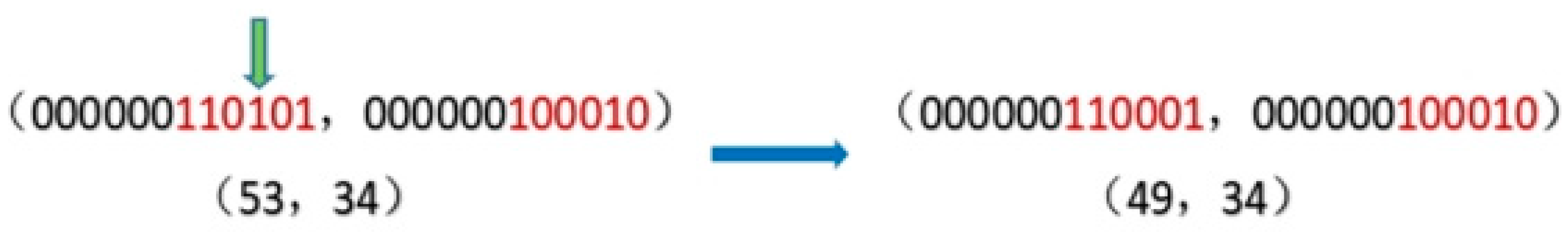
Step 2. Mutation Operation: To preserve population diversity and circumvent local optimum solutions, we introduced a mutation procedure subsequent to the crossover operation. This mutation process is carried out by randomly selecting specific bits and toggling their values. In particular, we randomly choose one bit from the lower six bits of the energy release source point coordinates and modify its value. The mutation probability is set at 0.04, indicating a 0.04 likelihood of undergoing a mutation procedure in each iteration. Through this approach, we can investigate new potential solutions while ensuring the stability of the overall region, leading to more refined optimization.

During the mutation process, we utilize a standard binary mutation strategy, that is, one bit is randomly selected from the lower six bits and toggled; if the bit is 0, it is changed to 1, and if it is 1, it is changed to 0. For example, assume that in a particular iteration, the new coordinates for the energy release source point obtained through the crossover operation are (55, 34). We randomly select the third bit of the x-coordinate (counting from the right) and change it from 1 to 0, resulting in new energy release source point coordinates of (49, 34). As shown in Figure 9, where the red part is the corresponding binary representation of the coordinates.

Through the integration of crossover and mutation operations, we can progressively converging to the global optimum solution. Furthermore, this optimization approach rooted in genetic algorithms showcases notable robustness and adaptability, rendering it apt for a variety of real-world applications.

Step 3. Energy Balancing Process: We incorporate the new coordinates for energy release points derived from the crossover and mutation operations and then initiate the energy balancing process. The specific steps of this process are delineated in Section 2.2.

Step 4. Iterative Optimization: We continuously execute the aforementioned steps to refine the positioning of the energy release points. This process continues until the current energy release area satisfies Equation (4) and all boundaries meet the energy balance criteria. The specific process is shown in Figure 10.

This section outlines the distinct steps of the genetic algorithm optimization, including gene selection, crossover, mutation, and iteration, to ensure the logical flow and uniformity of the entire optimization procedure. Each phase of the process is meticulously executed, adhering to established rules and guidelines to uphold the scientific integrity and precision of the optimization.

2.4. Mathematical Model and Time Complexity Analysis

In the previous introduction, we elaborated on our algorithm steps. Now, we will present the mathematical model and algorithm complexity:

Building Model Representation: The architectural model can be visualized as an image, where each pixel represents an image unit. This image is represented by the matrix M, where M[i][j] represents a certain pixel. Initially, all points (M[i][j]) are set to 0.

Region Division: The image is divided into N regions; each region ${\mathbf{R}}_{\mathbf{i}}$ (i = 1, 2, …, N) has an energy release point ${\mathbf{E}}_{\mathbf{i}}$. The function f(i,j) is used to determine the region to which each pixel belongs; f(i,j) = k (k = 1, 2, …, N) means that the energy release point ${\mathbf{E}}_{\mathbf{i}}$ belongs to the region ${\mathbf{R}}_{\mathbf{k}}$.

Energy Release: The potential function V(${\mathbf{E}}_{\mathbf{i}}$,$\mathbf{R}$) describes the energy state of each energy release point, where $\mathbf{R}$ is the diffusion distance. In each iteration, each energy release point Ei releases energy according to V(${\mathbf{E}}_{\mathbf{i}}$, R). With each iteration, R increases by 0.25 m, corresponding to a pixel size, spreading in a ring shape affecting surrounding pixels, and setting the passed pixel M[i][j] = k, until the energy balance is reached at the adjacent region boundary.

Area Calculation: After each regional boundary energy balance, calculate the area of each region. The function A(${\mathbf{R}}_{\mathbf{k}}$) represents the area of region ${\mathbf{R}}_{\mathbf{k}}$, A(${\mathbf{R}}_{\mathbf{k}}$) = sum(f(i,j) = k).

Energy Balance Iteration Process: The function D(A_ current, A_ previous) represents the area difference in each iteration. If D(A_current, A_previous) satisfies Equation (3), the energy balance process concludes. Otherwise, the centroid coordinates of all the current regions are identified, all of the pixel points are set to M[i][j] = 0, they are used as new energy release points, and the energy release process is continued until the difference meets the criteria.

Maximum and Minimum Area Difference: By comparing the areas of all regions, the maximum and minimum areas are identified. Amax and Amin represent the maximum and minimum areas, respectively. If their difference satisfies Equation (4), the results are output and the algorithm is exited. Otherwise, the genetic algorithm is proceeded to. Genetic Algorithm: The regions with the maximum and minimum areas are found, and the coordinates of their center points are encoded into 12-bit binary numbers, each bit representing a distance of 0.25 m. Crossing and mutating are carried out at the lower six bits (representing a distance of 16 m) to obtain new center point coordinates.

Genetic Algorithm Iteration Process: The energy release and balance process is repeated until the area difference of all regions is within an acceptable range. Multiple iterations may be needed until the termination condition is met.

We proceed to analyze the algorithmic complexity, where M represents the total number of pixel points in a provided image. The initial step involves dividing the image into N regions. This operation, although involving N divisions, is contingent upon traversing all M pixel points, leading to a complexity of O(M). In the subsequent energy release phase, the complexity remains O(M), as each energy release point diffuses energy throughout the image, necessitating another complete traversal of pixel points. When energy levels at the borders of adjacent regions equalize, the energy balance iteration commences. With k iterations, the complexity escalates to O(kM). The process of area calculation, involving another round of pixel point traversal to identify and record coordinates of points with identical values, retains the O(M) complexity. Comparing preceding and succeeding area differences, alongside the maximum and minimum disparities across N regions, incurs a complexity of O(N). Calculating the central coordinates of each region during the energy balance phase sums to a complexity of O(M) + O(N). Given that M vastly outnumbers N, the prevailing complexity is O(M).

In the genetic algorithm stage, identifying central points in regions with maximum and minimum areas mirrors the earlier method, maintaining the O(M) complexity. The ensuing steps of encoding coordinates and performing crossover and mutation operations are executed at a constant O(1) complexity. Invoking the multi-source point energy balance for several iterations and assuming a genetic algorithm iteration count of P culminates in a complexity of O(P(M + 1+M)) = O(M).

Our algorithm, comprising an energy balance procedure and a genetic algorithm, yields a total time complexity of O(M). Please be aware that the iteration counts in both the energy balance procedure and the genetic algorithm are influenced by various factors, such as the initial position and the number of energy source points, among others. Often, this count serves as a constant. This detail will be further clarified in the upcoming experimental section. This chapter delves deeply into the sources and divisions of the dataset and unveils the processes involved in multi-source energy balancing and the improvements made to the enhanced genetic algorithm, along with the presentation of mathematical models and the algorithm complexity. In the following chapter, we will utilize different types of datasets to thoroughly disclose the experimental results after algorithm iterations.

3. Results

In the experiments, we set p1 in Equation (3) to 0.1 and p2 in Equation (4) to 0.15. Based on extensive experimentation and engineering experience, we believe that within this error margin, the algorithm can converge rapidly. Furthermore, the pronounced changes during the iterative process are observable, facilitating the demonstration of the algorithm’s stability and reliability.

Our experimental variables fall into three categories:

Shape and Size of Input Datasets: In real-world scenarios, different buildings often have distinct top-down shapes and sizes. We selected representative top-down views of buildings as our datasets. These include regular shapes such as U-shaped, T-shaped, and H-shaped shapes, as well as irregular shapes like polygons. Each shape is provided with varying areas, ensuring our experiments align closely with real-world applications and possess broad applicability.

Number of Energy Release Points: In practical applications, buildings with larger areas typically have more energy release points, while those with smaller areas have fewer. In our experiments, we designated varying numbers of energy release points based on the area of the different datasets, mirroring real-world scenarios.

Partitioning Strategy: We employed both uniform and random partitioning. The latter aligns more closely with real-world applications, where energy release points are randomly distributed across areas. Through algorithmic simulation, we aim to achieve a satisfactory final position, ensuring a balanced distribution of the area and energy diffusion. In our experiments, the number of partitioned regions matches the number of energy release points, meaning each region is assigned an initial energy release point.

Table 1. Experimental Initial Value Setup.

Dataset	Point Number	Total Area (k)	Total Area (m2)
H-shape	10	244	15,252
U-shape	6	104	6506
T-shape	9	134	8398
polygonal	46	1249	78,072

presents the initial number of energy release points for each dataset, the number of pixels in each dataset (in units of ‘k’), and their corresponding total areas (in square meters).

After determining the shape, the size of the dataset, and the number of energy release points, we divided them into two groups based on a specific strategy. One group calculated the initial energy release points after evenly dividing the area, while the other group determined the energy source points after randomly dividing the area and calculated the energy balance boundaries and areas. These procedures have been detailed in previous sections. To ensure the accuracy of the results, we used the same dataset for both random and uniform divisions.

Upon dividing the area and determining the initial energy release points, we commenced the execution of the algorithm. The steps were identical for both uniformly and randomly divided datasets. After achieving multi-source energy balance, some data already met our error range. However, for some areas, despite reaching an energy balance, there was a significant discrepancy in the sizes of different regions. In such cases, we initiated our improved genetic algorithm for optimization. The process concluded upon meeting the set conditions, outputting the results.

We will showcase our experimental results in the following sections. In Section 3.1, we will showcase the iterative processes for the U-shaped, H-shaped, T-shaped, and polygonal datasets using both uniform and random segmentation strategies. In Section 3.2, we conducted ten experiments, tallying the number of equilibrium iterations and the number of iterations in the genetic algorithm for each experiment. Additionally, we used a line chart to display the ratio of the maximum to minimum area differences in the ten experiments. It is worth noting that our experimental procedure involves multiple iterations, with each iteration producing a corresponding result diagram. We have selected and displayed diagrams from the iterations that depict significant changes and represent the entire process. In the images we presented, the small circles represent the positions of the energy release points determined each time. In the image annotations, all images marked with ‘GA’ indicate that these are result images from iterations within the genetic algorithm.

3.1. The Iterative Process

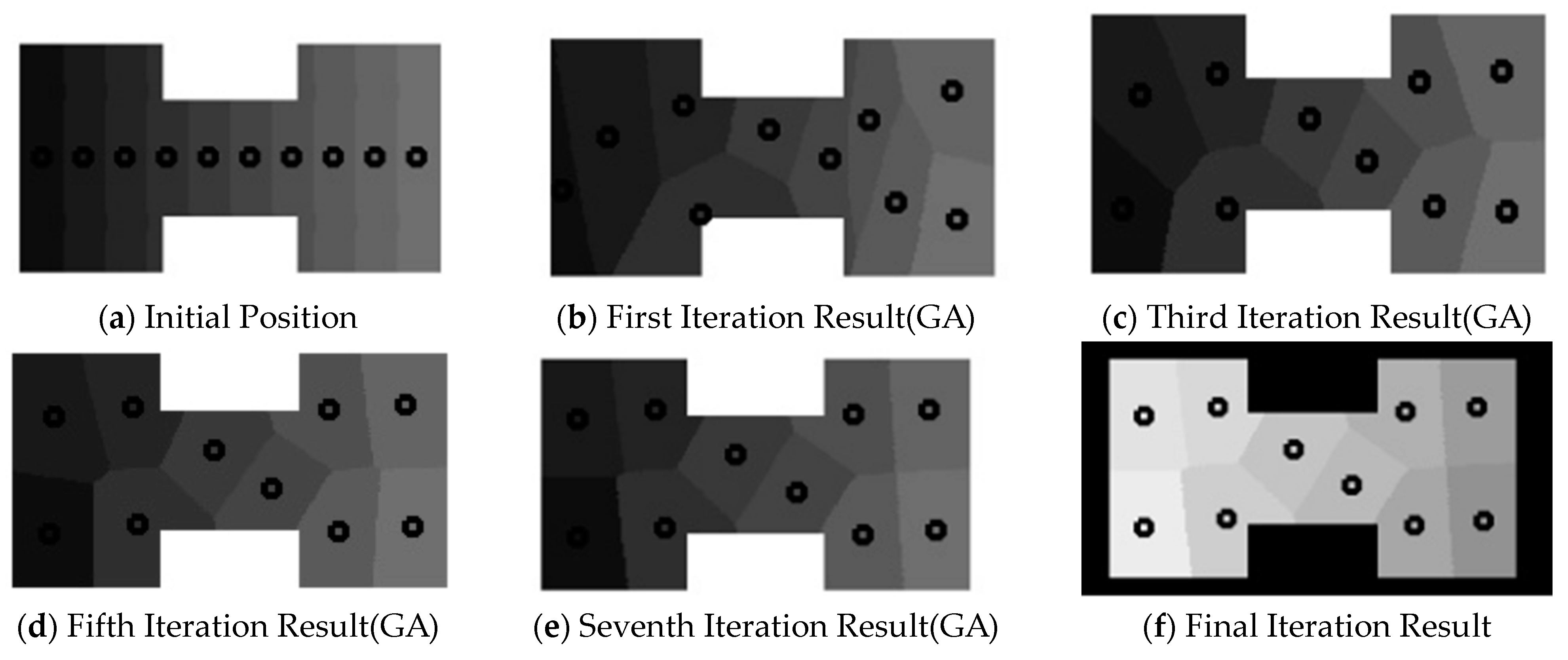
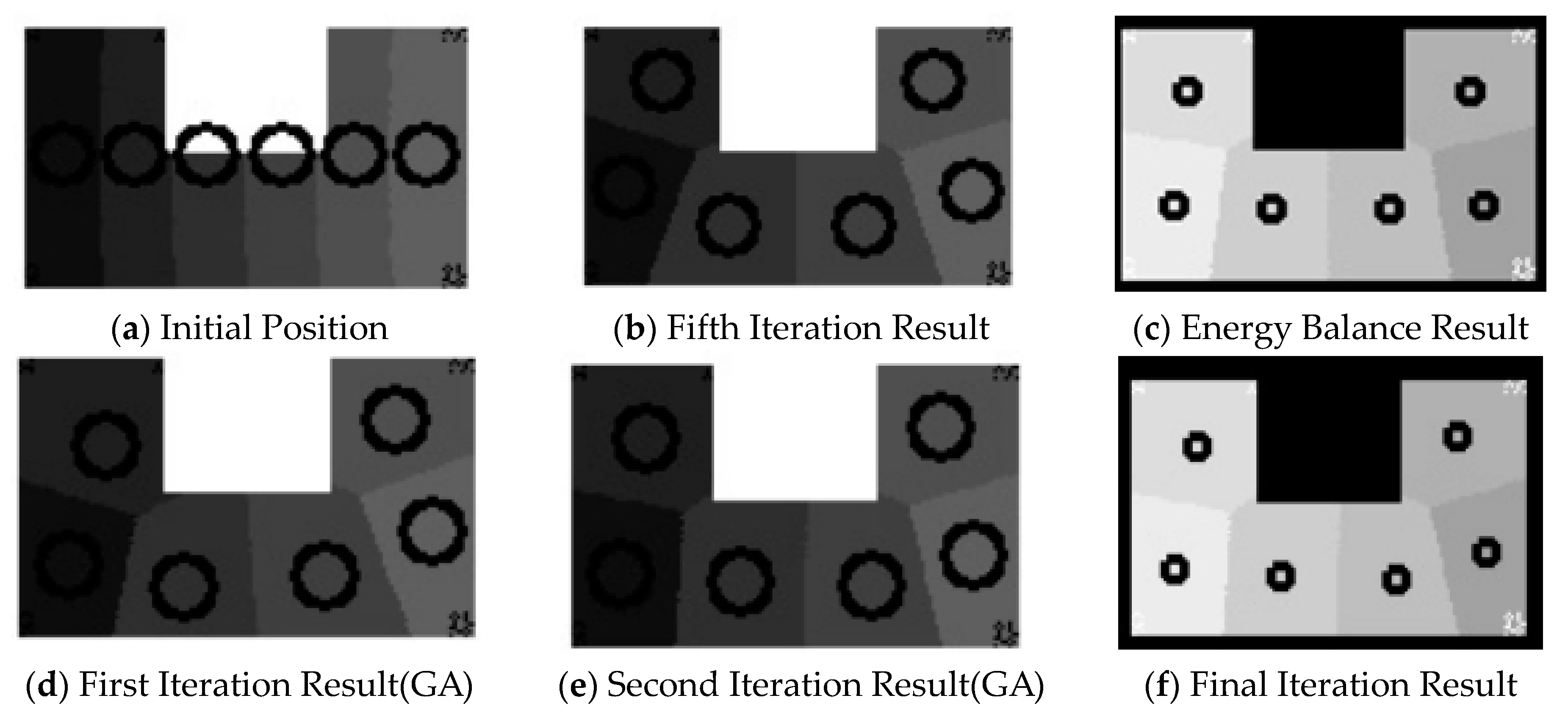
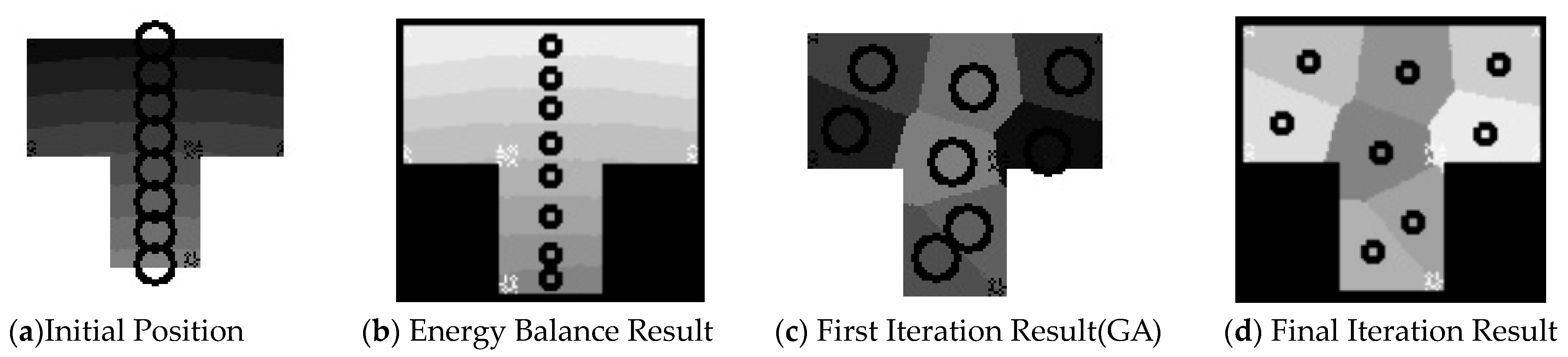
In Figure 11, the input for our algorithm is H-shaped data, with a given number of energy source points being 10. In Figure 11a, we vertically divided it into 10 regions, choosing the midpoint on the median line within each region as the initial energy release point. Due to the uniform spacing of the initial energy release points, we quickly reached a boundary energy balance state, but there was a noticeable disparity in region sizes at this point. Subsequently, the algorithm initiated the enhanced genetic algorithm. After seven iterations, the difference between the maximum and minimum area values fell within the allowable error range, outputting the final image. Figure 11b–e respectively display the results of the first, third, fifth, and last iterations. Figure 11f shows the final result of the data under equal division conditions. The dots within represent the final determined energy release points.

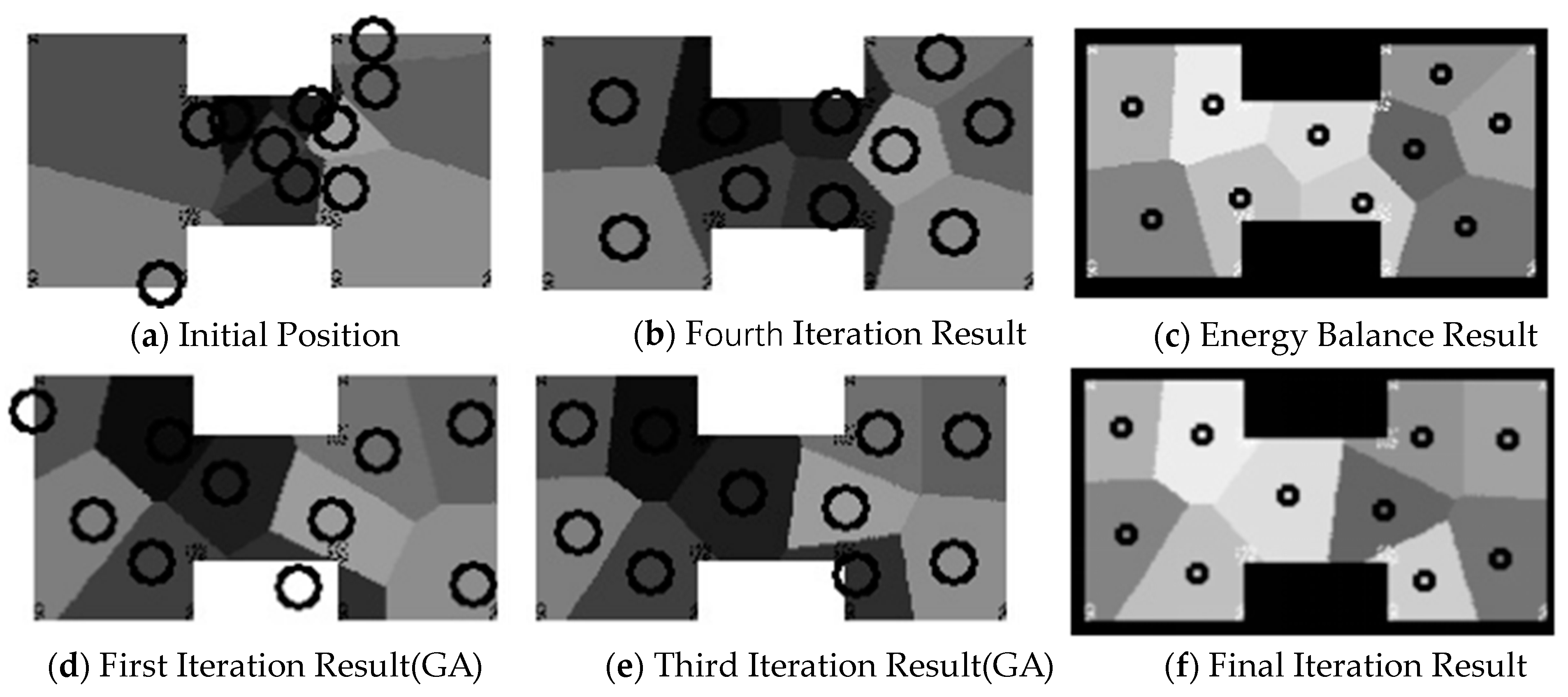
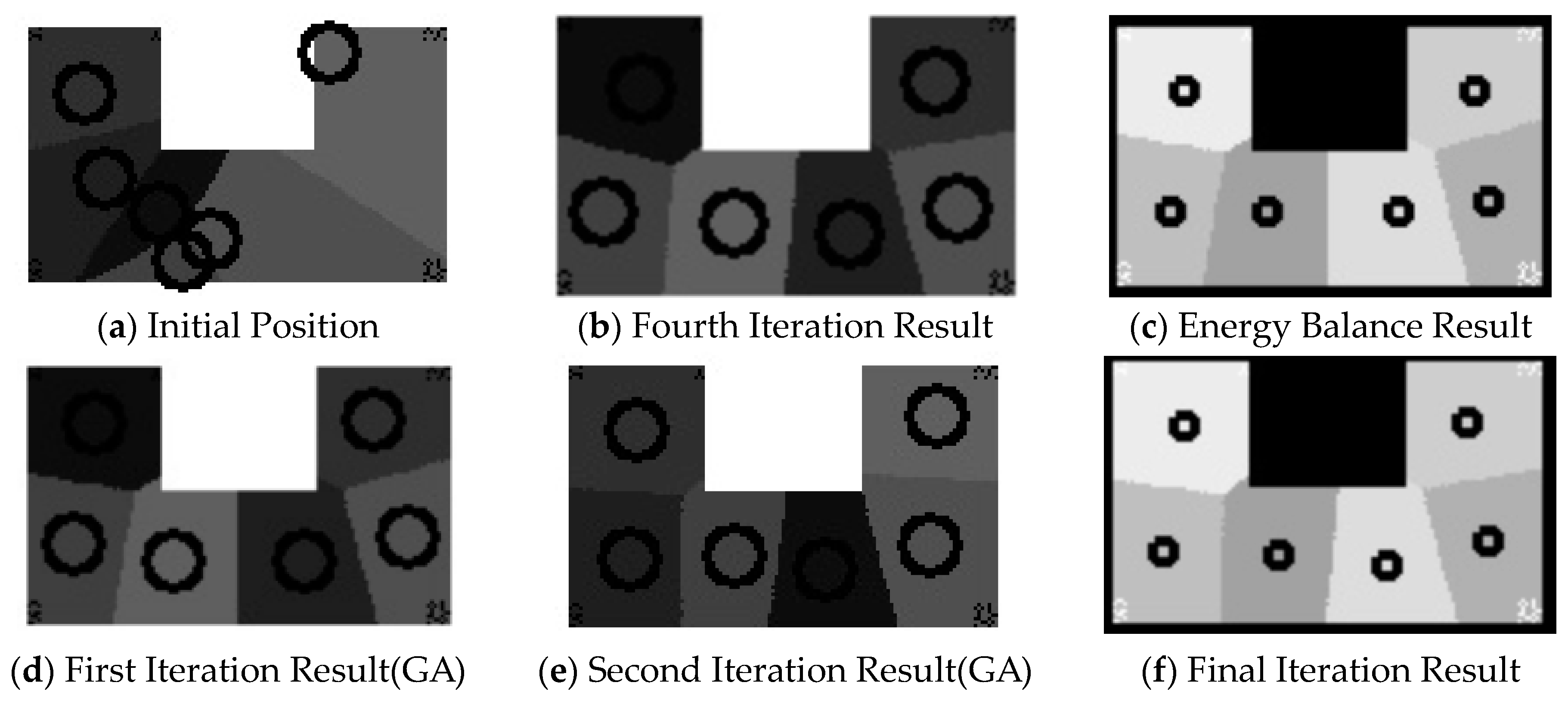
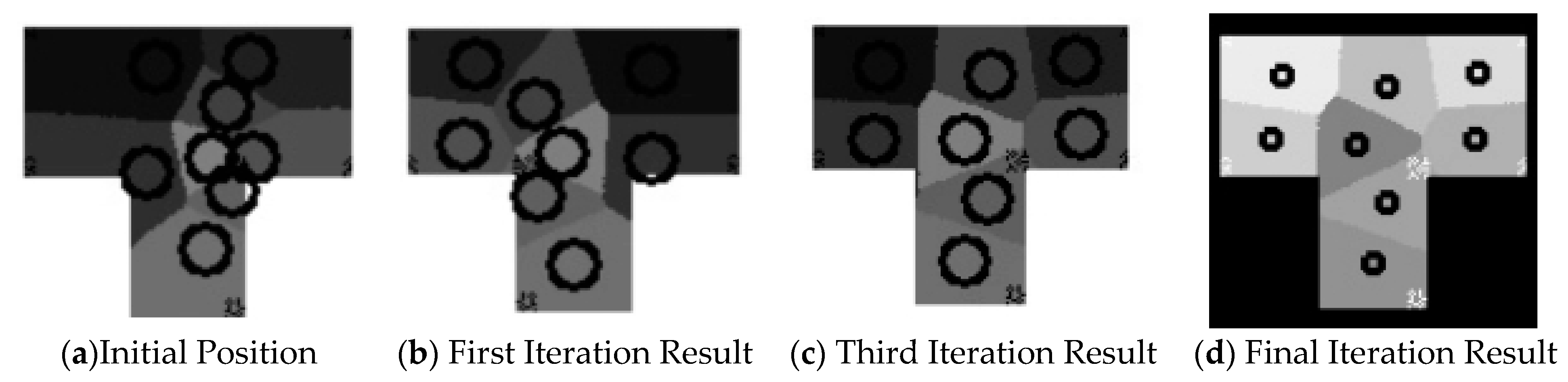
As observed in the iterative process above, the results are quite satisfactory after uniform segmentation. However, in real-world scenarios, we often tend to opt for a random segmentation strategy. As depicted in Figure 12a, we employed the same H-shaped data as mentioned above, dividing it randomly into ten parts and selecting ten initial energy release points at random. After eight iterations, the energy balance exit criteria were met, but there was a significant area difference. We then applied an improved genetic algorithm and, after six iterations, obtained the final results. Figure 12b illustrates the effect after the fourth iteration during the energy balance process, while Figure 12c displays the positions of the energy release points when energy balance was achieved. The first and third iteration effects of our improved genetic algorithm are shown in Figure 12d,e, respectively. Figure 12f presents the final confirmed positions.

Our experimental testing on the U-shaped dataset is presented in Figure 13. In Figure 13a, the initial energy source points are determined. After nine iterations of multi-source energy balancing, the difference between the maximum and minimum areas is still greater than 15%, hence the use of a genetic algorithm. Figure 13b,c respectively display the results after the fifth and final energy balancing iterations. As shown in Figure 13d,e in this experiment, the genetic algorithm was iterated twice, and Figure 13f outputs the final determined positions of the energy source points.

Similarly, we also randomly segmented the U-shaped data into six parts. In this experiment, the energy balance process was iterated six times, and the genetic algorithm was executed three times. Ultimately, we achieved a balanced energy boundary and an equal area distribution. In Figure 14, Figure 14a represents the initial random segmentation and random energy source point selection, while Figure 14b depicts the fourth iteration during the energy balance process. Figure 14c,f respectively show the output diagrams after multi-source energy balance and the completion of the genetic algorithm execution. Figure 14d,e illustrate the results of the first and second iterations of the genetic algorithm, respectively.

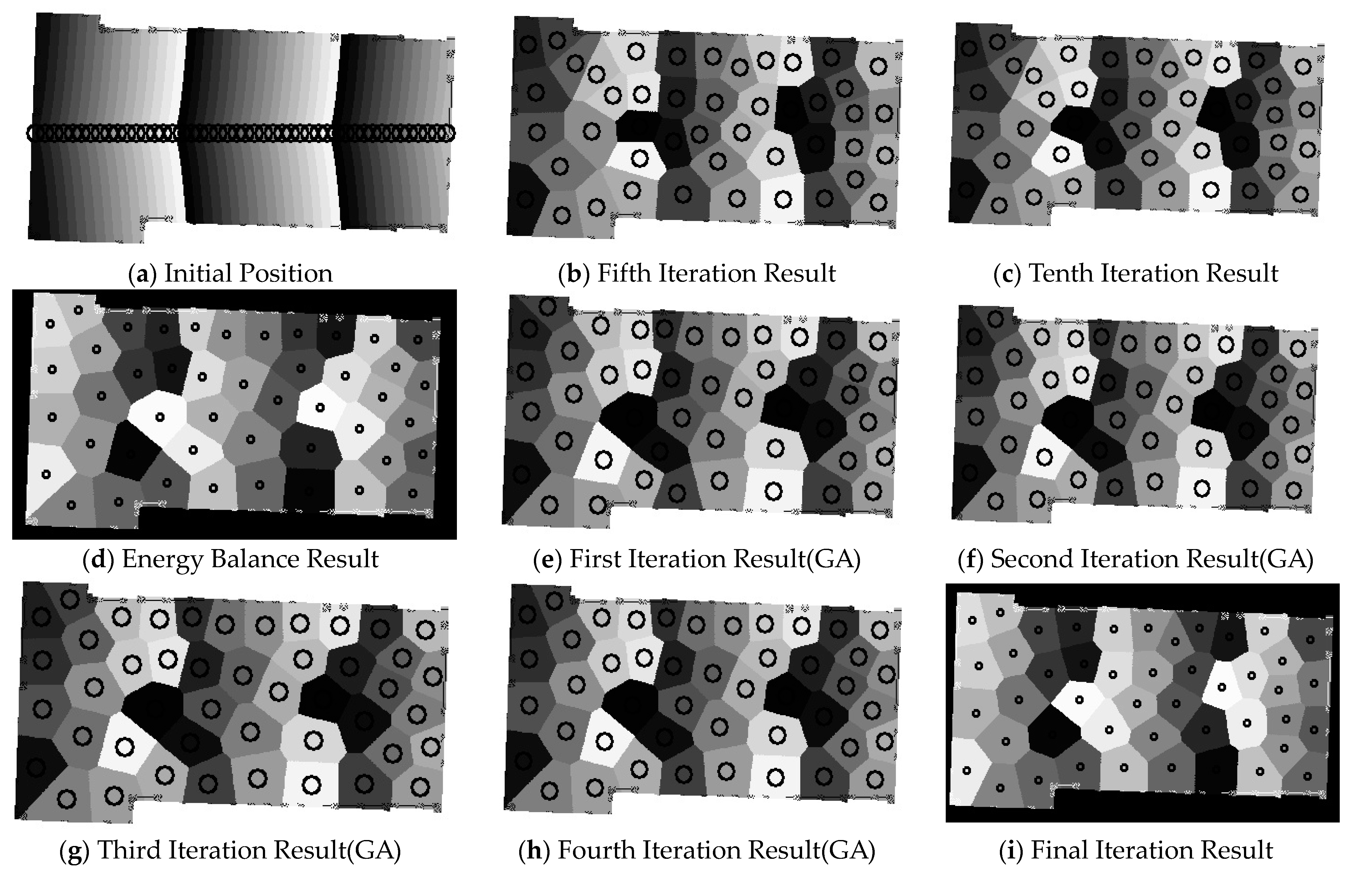
For polygonal data, We divided it equally into 46 parts, determined the initial energy release points, and proceeded with the iterations. During the energy balance process, there were a total of 17 iterations, while the genetic algorithm underwent 5 iterations. In Figure 15, Figure 15a still represents the initial random segmentation and random energy source point selection. Figure 15b depicts the fifth iteration during the energy balance process, and Figure 15c shows the tenth iteration. Figure 15d,i respectively illustrate the output diagrams after multi-source energy balance and the completion of the genetic algorithm execution. Figure 15e–h individually display the results of the first through fourth iterations of the genetic algorithm.

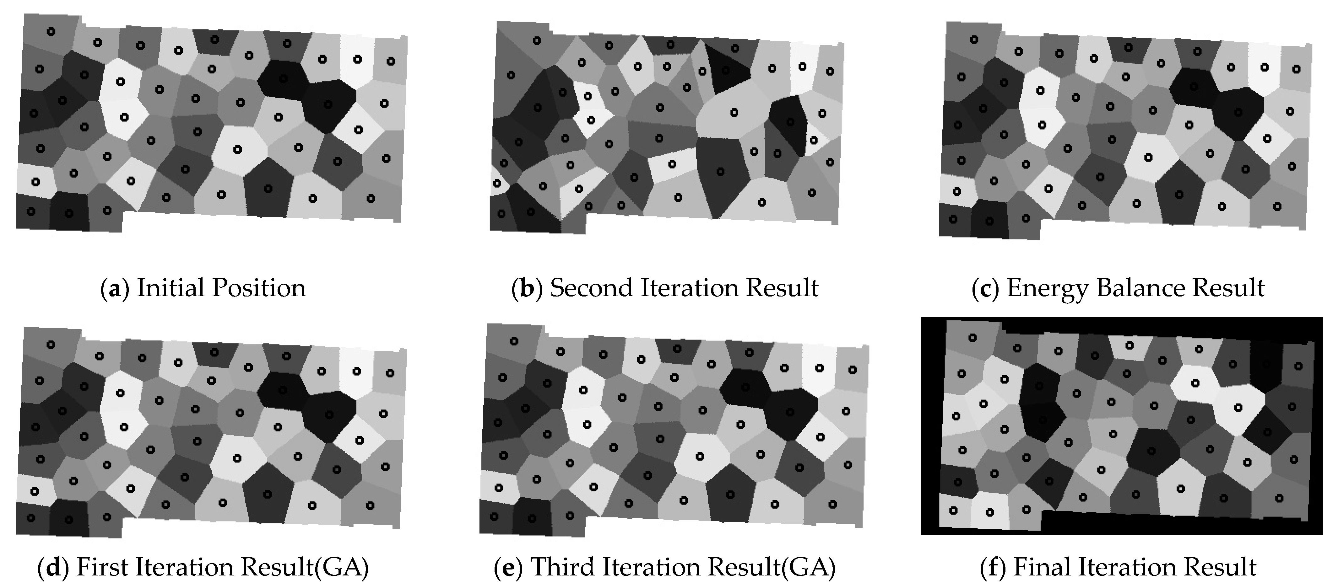
The random allocation of polygons is similar to the previous data allocation, where we randomly divided it into 46 parts and determined the initial energy release points. In this experiment, the energy balance process was iterated seven times, and the genetic algorithm was iterated five times. In Figure 16, Figure 16a represents the initial position diagram, Figure 16b describes the results of the second iteration during the energy balance process. Figure 16c,f represent the output diagrams after the execution of multi-source energy balance and the genetic algorithm, respectively. Figure 16d,e show the iteration diagrams for the first and third iterations of the genetic algorithm.

The T-shaped data exhibit similarities to the U-shaped data. Upon area equalization, the process quickly reaches energy balance, albeit with a significant area disparity, warranting the continued use of the genetic algorithm. In this experiment, we set the initial number of energy release points at eight, with the genetic algorithm iterating twice. The Figure 17 illustrates the progression: Figure 17a represents the initial state, Figure 17b showcases the result after energy balance, Figure 17c depicts the outcome of the first iteration of the genetic algorithm, and Figure 17d presents the final result.

For T-shaped data, after employing a random area allocation strategy, energy balance and area equalization can be achieved using the multi-source point energy balancing process, eliminating the need for further genetic algorithm execution. With a given energy source point count of eight, four iterations suffice to meet the experimental criteria. As illustrated in Figure 18, Figure 18a represents the initial state, Figure 18b,c depict the results after the first and third iterations, respectively, and Figure 18d displays the output after the final iteration.

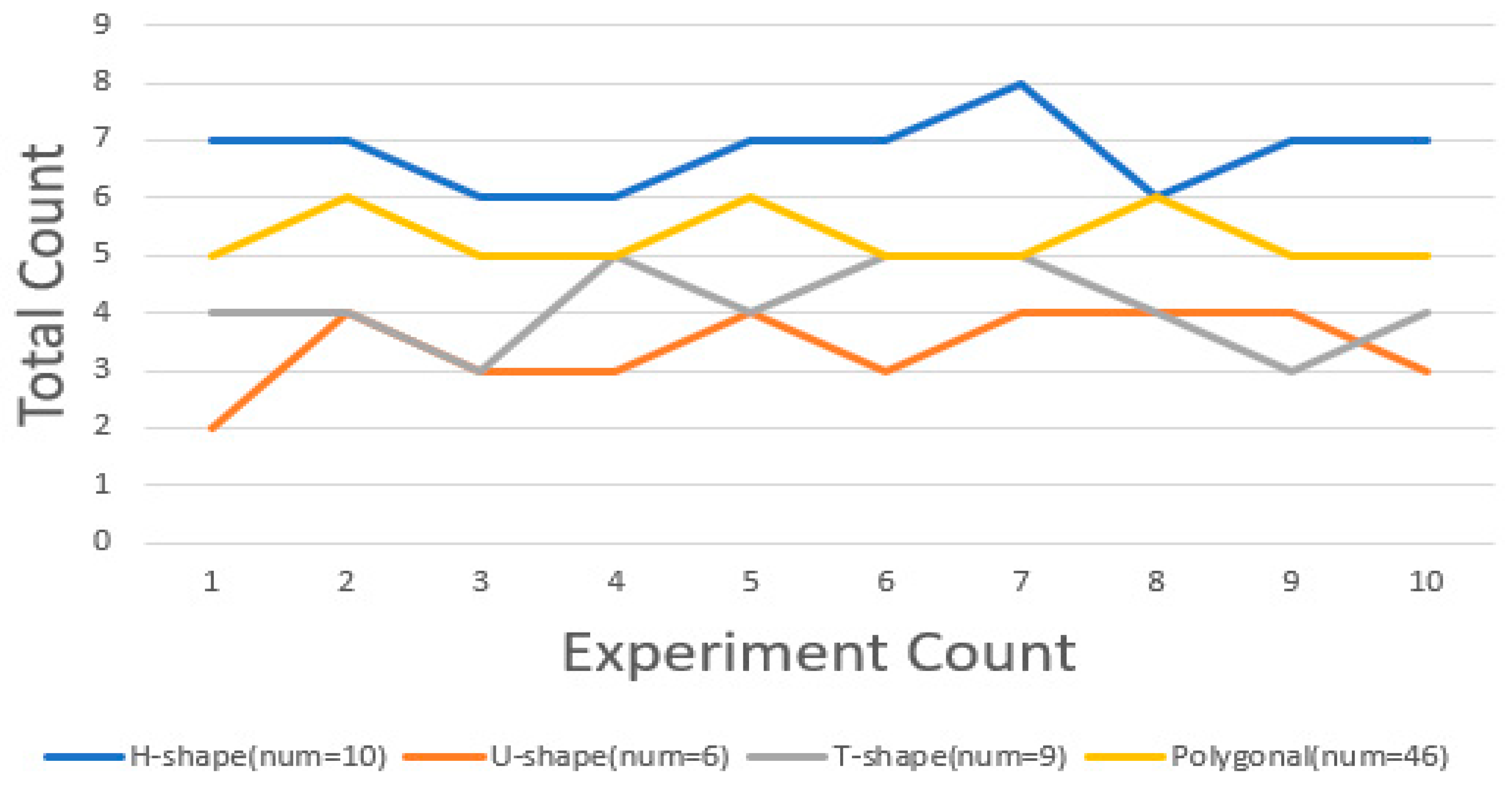
3.2. Stability Verification

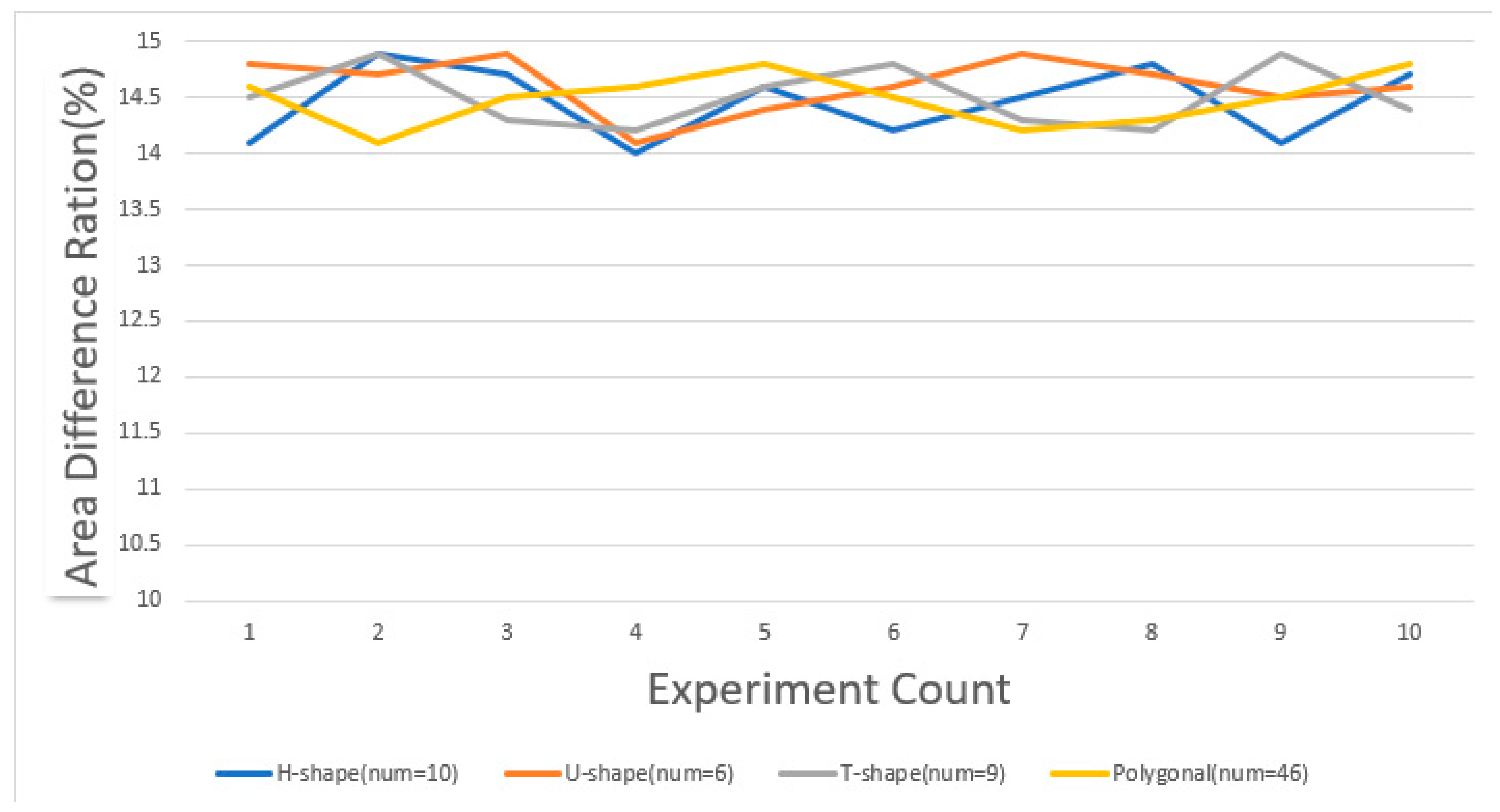
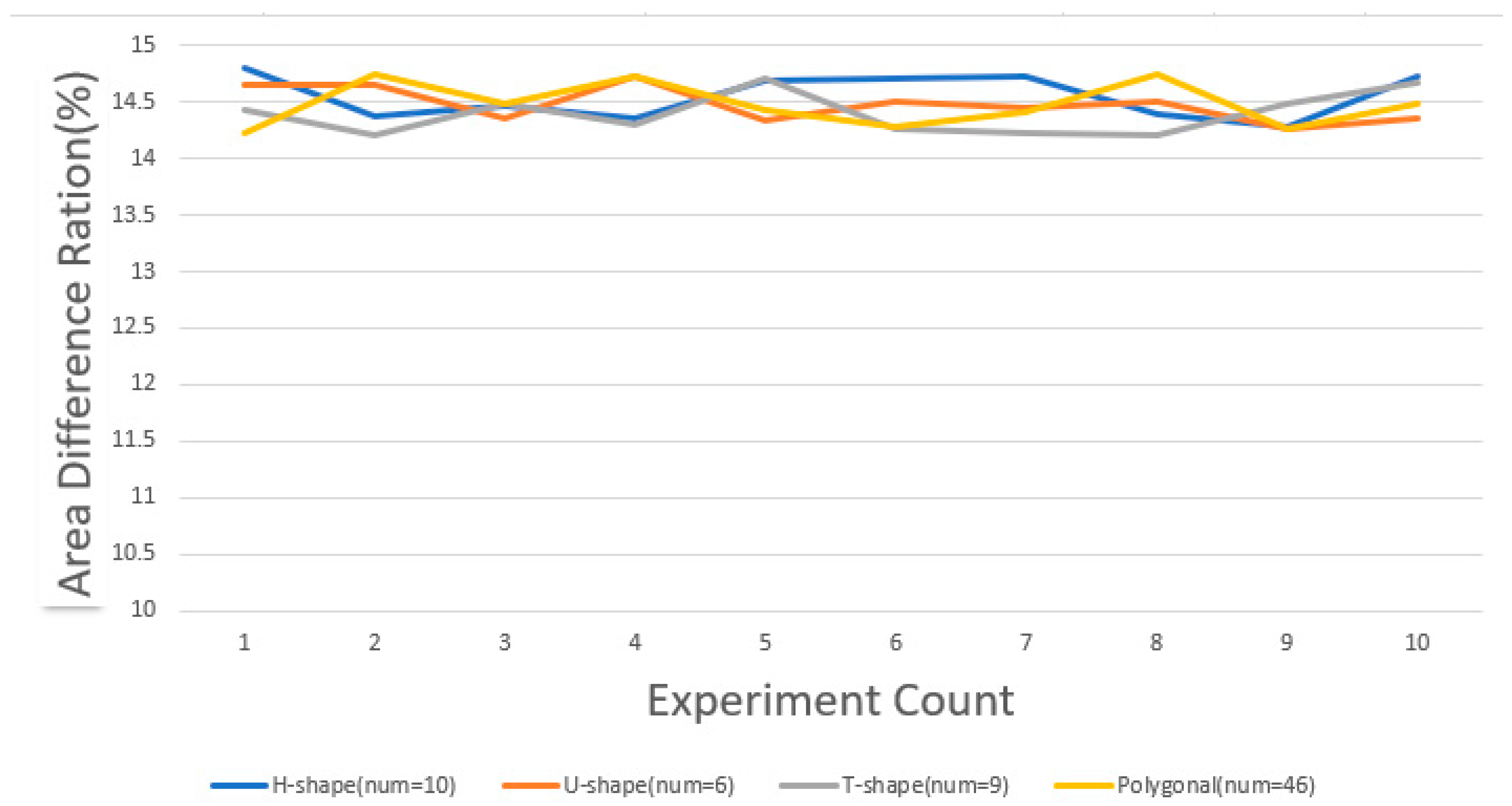
In this section, we conducted ten experiments to compare the area discrepancies under both the average allocation strategy and the random allocation strategy. Figure 19 illustrates the area discrepancy under the random allocation strategy, while Figure 20 depicts that under the average allocation strategy.

With the random allocation strategy, the discrepancy in the area is significantly associated with the initial position of the energy release point and the crossover mutation in the genetic algorithm, resulting in a larger fluctuation in its outcomes. In contrast, under the average allocation strategy, since the initial position of the energy release point remains constant, only minor differences emerge when random crossover and mutation are applied to the lower six digits of the central coordinates in the genetic algorithm. This explains the more stable discrepancy observed with the average allocation strategy.

Throughout the tests, the area discrepancy consistently remained within the range of 14–15%, aligning with our preset error threshold of 15%. These experiments robustly demonstrate the stability of our method.

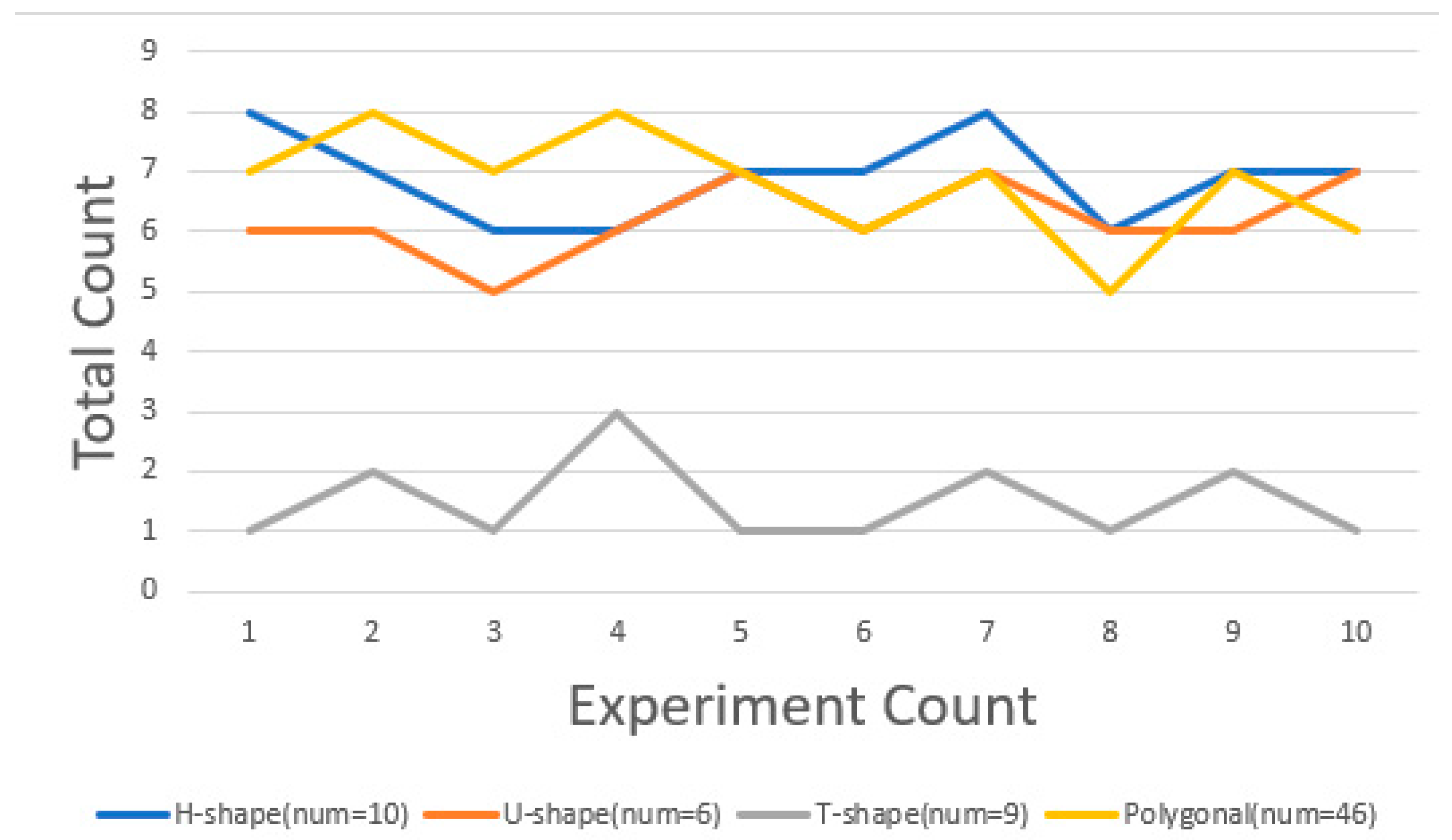
After quantifying the area discrepancies, the number of iterations also became a focal point of the study. We established specific area discrepancy objectives to reduce the number of iterations and rapidly achieve an area equilibrium.

In the average allocation strategy, for datasets with regular shapes, such as the U-shaped, T-shaped, and H-shaped datasets, we assigned the same initial positions in each dataset, all located at the center of the averagely divided area. Therefore, they can quickly achieve an energy equilibrium. However, in the genetic algorithm segment, since our ultimate goal is to have area discrepancies within the predetermined threshold, this is closely related to the shape of the dataset. For U-shaped, H-shaped, and T-shaped data, although they can quickly reach an energy balance, the area discrepancy is often larger, necessitating multiple iterations of the genetic algorithm. Generally, the more regular the shape, the quicker the genetic algorithm can achieve area balance. Due to the fixed starting point position in the average distribution strategy, the number of times energy equilibrium is achieved remains constant across multiple experiments. Therefore, under this strategy, we present the iteration count of the genetic algorithm. Figure 21 illustrates the number of times the genetic algorithm is executed under this strategy.

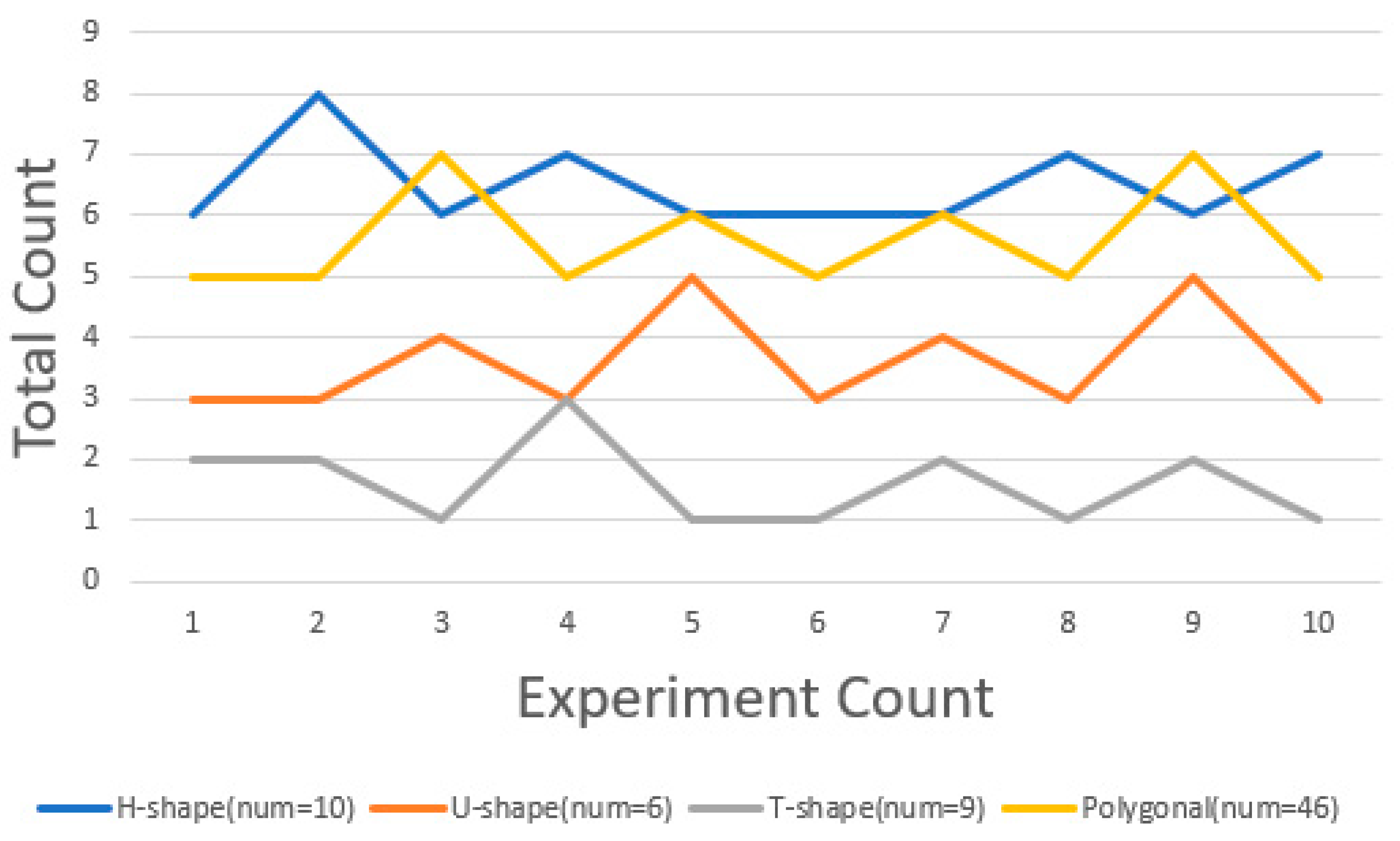
In the random allocation strategy, the initial energy release points are random, making the number of iterations unpredictable and necessitating empirical data for calculation. Generally, the more dispersed the initial energy release points are, the easier it is to quickly reach energy balance. Notably, in some irregular shapes like polygons, randomly assigned energy release points typically lead to a quicker energy balance, as points in irregular shapes are more likely to be evenly dispersed under the random allocation strategy. In the genetic algorithm segment, for regular-shaped data like U-shaped, H-shaped, and T-shaped data, after achieving energy balance, the area discrepancies in different regions are usually smaller, and hence, fewer iterations of the genetic algorithm are required. The Figure 22 and Figure 23 shows the statistics of the energy balance and genetic algorithm iteration numbers for different datasets over the ten experiments we conducted.

In the above figure, we can observe that regardless of the scenario, the difference in our iteration counts does not exceed three times. This demonstrates that our algorithm requires fewer iterations, and the area discrepancy also lies between 14 and 15%, which aligns with our expectations.

Our experiment elaborately discusses the energy balance iteration process and the improved genetic algorithm iteration process under different strategies for H-shaped, U-shaped, T-shaped, and polygonal configurations. The experiment demonstrates that our method yields smaller error margins and requires fewer iterations, effectively addressing the issue of energy and area imbalance in multi-source point energy release scenarios. The experimental results are compelling and present a strong case for the efficacy of our proposed method.

4. Conclusions

In this study, we introduce an innovative approach in the field of building demolition. This method involves placing multiple initial energy source points on various building models and utilizing the point energy release shockwave overpressure formula as the potential function for energy diffusion. When the energy at the diffusion boundaries becomes equal, and there are significant differences in diffusion areas in different regions, we employ an enhanced genetic algorithm for optimization. This is followed by another energy balancing process. This iterative process is repeated until the final energy equilibrium is achieved, ensuring that the disparity between the maximum and minimum areas falls within an acceptable range.

In the experimental section, we provide various partitioning strategies and numbers of energy release points for different building models. We present corresponding iteration graphs and final release point location determination graphs. From these visuals, we can observe that our results are quite satisfactory, with areas in various regions being relatively close. Furthermore, through multiple algorithm simulation tests on models resembling real building types, we record the number of iterations and the maximum–minimum area differences. This demonstrates that our method can achieve fewer iterations and smaller area differences, exhibiting good stability and significant practical utility. In everyday life, this research outcome can offer a more scientific and efficient approach to building demolition. By optimizing the distribution of energy source points and the energy diffusion process, it becomes possible to more accurately control the scope and effectiveness of building demolition, thereby enhancing safety and efficiency in demolition work.

Our current research primarily focuses on energy diffusion points with the same underlying function. In future research, we plan to explore the iterative process with multiple energy release points with different potential functions and address the issue of energy superposition when release points are in close proximity.