
An Image Denoising Technique Using Wavelet-Anisotropic Gaussian Filter-Based Denoising Convolutional Neural Network for CT Images
Abstract
:1. Introduction
Main Contribution
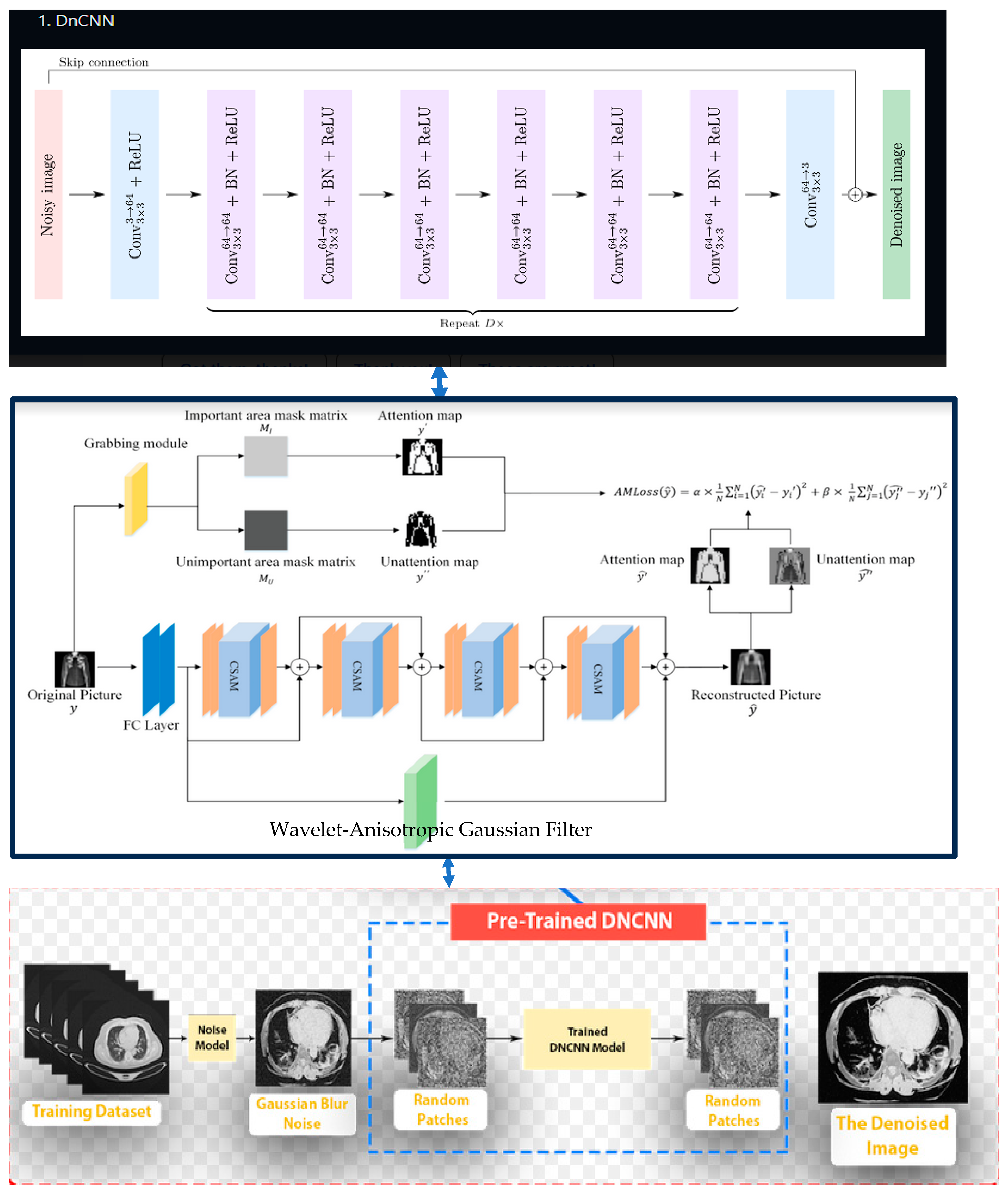
- An ensemble approach is proposed using DnCNN, the anisotropic Gaussian filter (AGF), and Haar wavelet transform. The AGF and Haar transform are applied as preprocessing operations. The choice of AGF was primarily due to its adaptability to edge orientation, adaptive filtering, and directional information, effectively handling edges based on gradient magnitude and preventing blurring along edges commonly encountered with standard filters.
- The ensemble approach demonstrates better results when compared to CNN-based methods and other standard spatial filtering techniques in reducing the blurring effect and improving image quality and restoration.
2. Related Work
3. Methodology
- Step 1 (input original image): read authentic CT scan images.
- Step 2 (perform initial noise detection): Use the anisotropic Gaussian filter (AGF) to gauge the level of Gaussian noise in the initial test when checking for the type of noise in the images. It smoothens images while preserving the edges and details, effectively reducing noise levels.
- Step 3 (add Gaussian blur noise): read noisy corrupted CT scan images.
- Step 4 (perform DnCNN): the general CNN process is given below:
- Design a denoising CNN with skip connections to preserve low-level image details during denoising.
- Implement batch normalization and ReLU activation after each convolutional layer to improve training stability.
- Use residual blocks to capture and learn essential image features.
- Implement skip connections to pass relevant information across different layers.
- Step 5 (perform denoising):
- Apply the designed CNN to each detail sub-band obtained from the wavelet decomposition (LH, HL, HH).
- Set the denoising threshold for each sub-band based on the noise level (σ) obtained in the preprocessing step. For example, set the point as 0.1. The threshold value is a determinant of the image used for the experiments, and in this study, a value of 0.05 was used. The value was chosen to demonstrate the concept of thresholding and its impact on image denoising. Factors such as noise characteristics and specific image content should be empirically determined in an experiment.
- Perform soft thresholding on the CNN output for each sub-band to reduce noise and preserve critical features.
- Denoising uses soft thresholding on the CNN output for each detail sub-band. The soft thresholding formula for denoising a sub-band is given by:
- C_denoised (i, j) = sign (C(i, j)) ∗ max(|C(i, j)| − λ, 0)
- Where C_denoised (i, j) are the denoised DWT coefficients, C(i, j) are the original DWT coefficients, and λ is the wavelet threshold.
- Denoising threshold: the denoising threshold (λ) is a parameter that determines the level at which noisy coefficients in each sub-band will be attenuated or suppressed during the denoising process.
- Noise level (σ): The noise level (σ) represents the standard deviation of the noise present in the image. It characterizes the amount of noise contamination in the image, such as Gaussian blur noise.
- Relationship: The denoising threshold (λ) is typically set based on each sub-band’s estimated noise level (σ). The choice of the denoising threshold is critical because it determines which coefficients are considered noise and should be reduced or eliminated.
- If λ is set too high, it may remove essential image details, leading to over-smoothing and loss of image information.
- If λ is too low, it may not effectively suppress the noise, resulting in noisy artifacts in the denoised image.
- Step 6 (Haar wavelet transform)
- Step 7 (inverse wavelet transform):
- Combine the denoised detail sub-bands with the original approximation sub-band.
- Perform the 2D inverse discrete wavelet transform (IDWT) to reconstruct the final denoised CT image.
- The 2D IDWT combines the denoised detail sub-bands with the original approximation sub-band to reconstruct the final denoised CT image.
4. Experimental Results and Analysis
4.1. Dataset
4.2. Hyperparameters
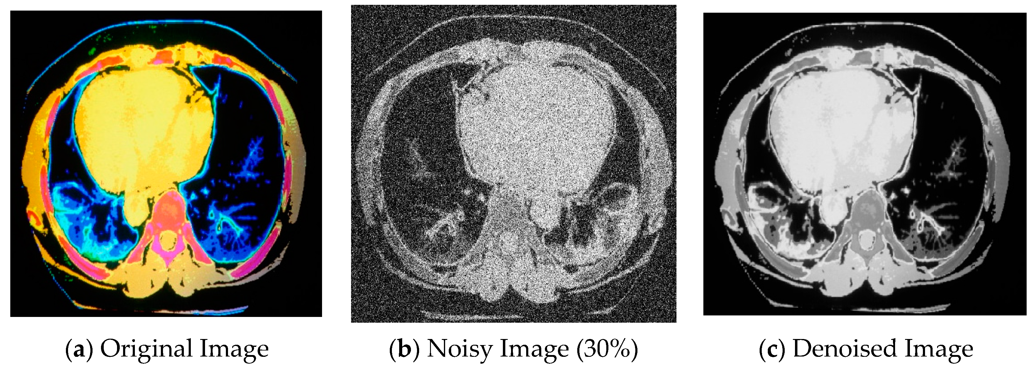
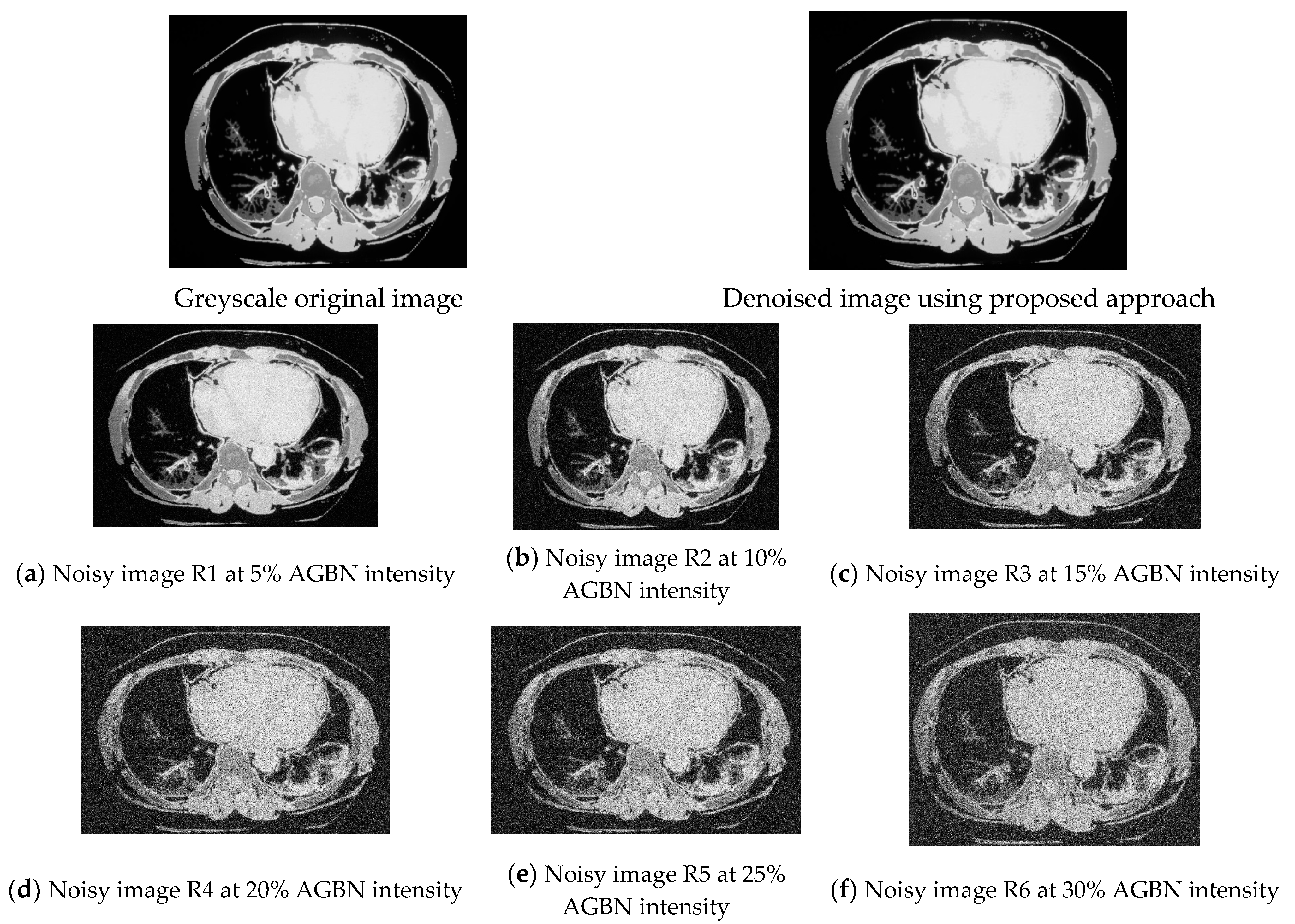
4.3. Qualitative Analysis
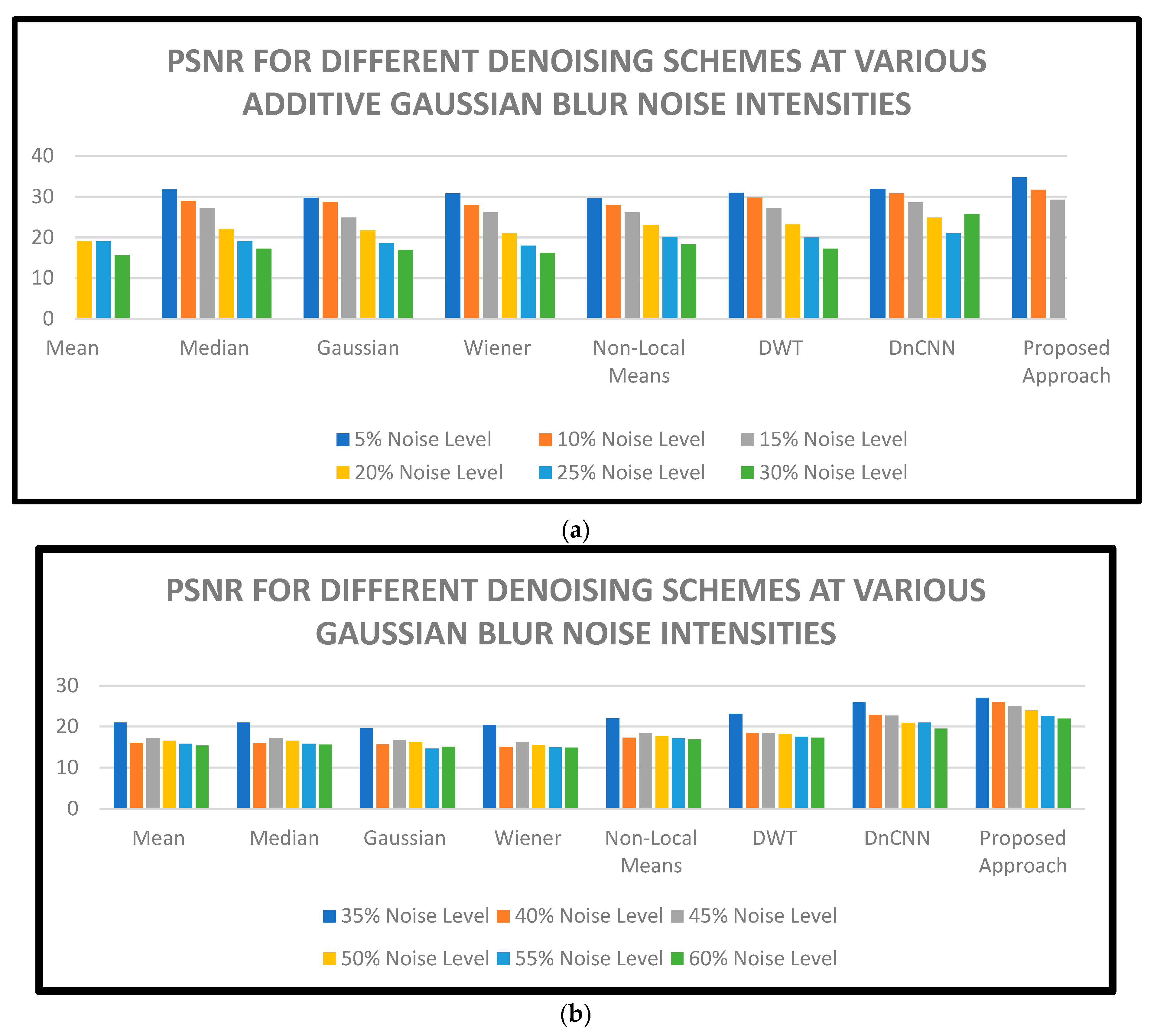
4.4. Quantitative Analysis
4.5. Quantitative Results
5. Discussion
6. Conclusions
Author Contributions
Funding
Institutional Review Board Statement
Informed Consent Statement
Data Availability Statement
Conflicts of Interest
References
- Alanazi, T.M.; Berriri, K.; Albekairi, M.; Ben Atitallah, A.; Sahbani, A.; Kaaniche, K. New Real-Time High-Density Impulsive Noise Removal Method Applied to Medical Images. Diagnostics 2023, 13, 1709. [Google Scholar] [CrossRef]
- Tian, C.; Fei, L.; Zheng, W.; Xu, Y.; Zuo, W.; Lin, C.W. Deep learning on image denoising: An overview. Neural Netw. 2020, 131, 251–275. [Google Scholar] [CrossRef] [PubMed]
- Kadhim, M.A. Restoration Medical Images from Speckle Noise Using Multifilters. In Proceedings of the 2021 7th International Conference on Advanced Computing and Communication Systems (ICACCS), Coimbatore, India, 19–20 March 2021; Volume 1, pp. 1958–1963. [Google Scholar]
- Satra, H.; Gupta, A. Lung Nodule Detection using Segmentation Approach for Computed Tomography Scan Images. Int. J. Forresearch Appl. Sci. Eng. Technol. 2021, 9, 1778–1790. [Google Scholar] [CrossRef]
- Das, K.P.; Chandra, J. A Review on Preprocessing Techniques for Noise Reduction in PET-CT Images for Lung Cancer. In Congress on Intelligent Systems: Proceedings of CIS 2021; Springer Nature: Singapore, 2022; Volume 2, pp. 455–475. [Google Scholar]
- Choi, H.; Jeong, J. Despeckling algorithm for removing speckle noise from ultrasound images. Symmetry 2020, 12, 938. [Google Scholar] [CrossRef]
- Bharati, S.; Khan, T.Z.; Podder, P.; Hung, N.Q. A comparative analysis of image denoising problem: Noise models, denoising filters and applications. In Cognitive Internet of Medical Things for Smart Healthcare: Services and Applications; Springer: Berlin/Heidelberg, Germany, 2021; pp. 49–66. [Google Scholar]
- Rausch, I.; Mannheim, J.G.; Kupferschläger, J.; la Fougère, C.; Schmidt, F.P. Image quality assessment along the one-metre axial field-of-view of the total-body Biograph Vision Quadra PET/CT system for 18F-FDG. Ejnmmi Phys. 2022, 9, 87. [Google Scholar] [CrossRef]
- Goyal, B.; Agrawal, S.; Sohi, B.S. Noise issues prevail in various types of medical images. Biomed. J. 2018, 11, 1227. [Google Scholar]
- Florez-Aroni, S.M.; Hancco-Condori, M.A.; Torres-Cruz, F. Noise Reduction in Medical Images. arXiv 2023, arXiv:2301.01437. [Google Scholar]
- Bhonsle, D.; Bagga, J.; Mishra, S.; Sahu, C.; Sahu, V.; Mishra, A. Reduction of Gaussian noise from Computed Tomography Images using Optimized Bilateral Filter by Enhanced Grasshopper Algorithm. In Proceedings of the 2022 Second International Conference on Advances in Electrical, Computing, Communication and Sustainable Technologies (ICAECT), Bhilai, India, 21–22 April 2022; pp. 1–9. [Google Scholar]
- Hermena, S.; Young, M. CT-scan image production procedures. In StatPearls [Internet]; StatPearls Publishing: Treasure Island, FL, USA, 2022. [Google Scholar]
- Nakamura, Y.; Higaki, T.; Tatsugami, F.; Honda, Y.; Narita, K.; Akagi, M.; Awai, K. Possibility of deep learning in medical imaging focusing on improvement of computed tomography image quality. J. Comput. Assist. Tomogr. 2020, 44, 161–167. [Google Scholar] [CrossRef]
- Kaur, A.; Dong, G. A Complete Review on Image Denoising Techniques for Medical Images. Neural Process Lett. 2023, 55, 7807–7850. [Google Scholar] [CrossRef]
- Mehta, D.; Padalia, D.; Vora, K.; Mehendale, N. MRI image denoising using U-Net and Image Processing Techniques. In Proceedings of the 2022 5th International Conference on Advances in Science and Technology (ICAST), Mumbai, India, 2–3 December 2022; pp. 306–313. [Google Scholar]
- Xu, J.; Gong, E.; Ouyang, J.; Pauly, J.; Zaharchuk, G. Ultra-low-dose 18F-FDG, brain PET/MR denoising, using deep learning and multi-contrast information. In Medical Imaging 2020: Image Processing; SPIE: Bellingham, WA, USA, 2020; Volume 11313, pp. 420–432. [Google Scholar]
- Kim, B.; Han, M.; Shim, H.; Baek, J. Performance comparison of convolutional neural network-based image denoising methods: The effect of loss functions on low-dose CT images. Med. Phys. 2019, 46, 3906–3928. [Google Scholar] [CrossRef]
- Sagheer, S.V.M.; George, S.N. A review on medical image denoising algorithms. Biomed. Signal Process. Control 2020, 61, 102036. [Google Scholar]
- Kaur, J.; Goyal, B.; Dogra, A. An Analysis of Different Noise Removal Techniques in Medical Images. In Advances in Signal Processing, Embedded Systems, and IoT: Proceedings of Seventh ICMEET-2022; Springer Nature: Singapore, 2023; pp. 579–590. [Google Scholar]
- Thakur, R.S.; Chatterjee, S.; Yadav, R.N.; Gupta, L. Medical image denoising using convolutional neural networks. In Digital Image Enhancement and Reconstruction; Academic Press: Cambridge, MA, USA, 2023; pp. 115–138. [Google Scholar]
- Abdelhamed, A.; Timofte, R.; Brown, M.S. Ntire 2019 challenge on actual image denoising: Methods and results. In Proceedings of the IEEE/CVF Conference on Computer Vision and Pattern Recognition Workshops, Long Beach, CA, USA, 16–20 June 2019; pp. 1–14. [Google Scholar]
- Vimala, C.; Aruna Priya, P.; Subramani, C. Wavelet transform approach for image processing–A research motivation for engineering graduates. Int. J. Electr. Eng. 2021, 58, 373–384. [Google Scholar] [CrossRef]
- Zhang, X. A modified non-local means using bilateral thresholding for image denoising. Multimed. Tools Appl. 2023, 1–22. [Google Scholar] [CrossRef]
- Mayasari, R.; Heryana, N. Reduce Noise in Computed Tomography Images using Adaptive Gaussian Filter. arXiv 2019, arXiv:1902.05985. [Google Scholar]
- Ştefănigă, S.A. Fine-Tuned Medical Images Denoising using Median Filtering. Appl. Med. Inform. 2021, 43, 27. [Google Scholar]
- Juneja, M.; Joshi, S.; Singla, N.; Ahuja, S.; Saini, S.K.; Thakur, N.; Jindal, P. Denoising of computed tomography using bilateral median-based autoencoder network. Int. J. Imaging Syst. Technol. 2022, 32, 935–955. [Google Scholar] [CrossRef]
- Ismael, A.A.; Baykara, M. Digital Image Denoising Techniques Based on Multi-resolution Wavelet Domain with Spatial Filters: A Review. Trait. Du Signal 2021, 38, 639–651. [Google Scholar] [CrossRef]
- Anam, C.; Adi, K.; Sutanto, H.; Arifin, Z.; Budi, W.S.; Fujibuchi, T.; Dougherty, G. Noise reduction in CT images using a selective mean filter. J. Biomed. Physicsengineering 2020, 10, 623. [Google Scholar] [CrossRef]
- Diwakar, M.; Singh, P. CT image denoising using the multivariate model and its method of noise thresholding in the non-subsampled shearlet domain. Biomed. Signal Process. Control 2020, 57, 101754. [Google Scholar] [CrossRef]
- Sumijan, S.S.; Purnama, A.W.; Arlis, S. Peningkatan Kualitas Citra CT-Scan dengan Penggabungan Metode Filter Gaussian dan Filter Median. J. Teknol. Inf. Dan Ilmu Komput. 2019, 6, 591–600. [Google Scholar] [CrossRef]
- Chillaron, M.; Vidal, V.; Verdu, G. Evaluation of image filters for their integration with LSQR computerized tomography reconstruction method. PLoS ONE 2020, 15, e0229113. [Google Scholar] [CrossRef]
- El-Shafai, W.; Mahmoud, A.; Ali, A.; El-Rabaie, E.; Taha, T.; Zahran, O.; El-Fishawy, A.S.; Soliman, N.F.; Alhussan, A.A.; Abd El-Samie, F. Deep cnn model for multimodal medical image denoising. Comput. Mater. Contin 2022, 73, 3795–3814. [Google Scholar] [CrossRef]
- Yue, Z.; Zhao, Q.; Zhang, L.; Meng, D. Dual adversarial network: Toward real-world noise removal and noise generation. In Proceedings of the Computer Vision–ECCV 2020: 16th European Conference, Glasgow, UK, 23–28 August 2020; Part X 16. Springer International Publishing: Berlin/Heidelberg, Germany; pp. 41–58. [Google Scholar]
- Xu, J.; Huang, Y.; Cheng, M.M.; Liu, L.; Zhu, F.; Xu, Z.; Shao, L. Noisy-as-clean: Learning self-supervised denoising from corrupted images. IEEE Trans. Image Process. 2020, 29, 9316–9329. [Google Scholar] [CrossRef] [PubMed]
- Aslam, M.A.; Munir, M.A.; Cui, D. Noise removal from medical images using hybrid filters of technique. J. Phys. Conf. Ser. 2020, 1518, 012061. [Google Scholar] [CrossRef]
- You, N.; Han, L.; Zhu, D.; Song, W. Research on image denoising in edge detection based on wavelet transform. Appl. Sci. 2023, 13, 1837. [Google Scholar] [CrossRef]
- Liang, H.; Zhao, S. Salt and Pepper Noise Suppression for Medical Image by Using Non-local Homogenous Information. In Cognitive Internet of Things: Frameworks, Tools and Applications; Springer: Cham, Switzerland, 2020; pp. 189–199. [Google Scholar]
- Garg, B. Restoration of highly salt-and-pepper-noise-corrupted images using a novel adaptive trimmed median filter. Signal Image Video Process. 2020, 14, 1555–1563. [Google Scholar] [CrossRef]
- Gupta, S.; Sunkaria, R.K. Real-time salt and pepper noise removal from medical images using a modified weighted average filtering. In Proceedings of the 2017 the Fourth International Conference on Image Information Processing (ICIIP), Shimla, India, 21–23 December 2017; pp. 1–6. [Google Scholar]
- Usui, K.; Ogawa, K.; Goto, M.; Sakano, Y.; Kyougoku, S.; Daida, H. Quantitative evaluation of deep convolutional neural network-based image denoising for low-dose computed tomography. Vis. Comput. Ind. Biomed. Art 2021, 4, 21. [Google Scholar] [CrossRef]
- Kim, B.G.; Kang, S.H.; Park, C.R.; Jeong, H.W.; Lee, Y. Noise level and similarity analysis for computed tomographic thoracic image with fast non-local means denoising algorithm. Appl. Sci. 2020, 10, 7455. [Google Scholar] [CrossRef]
- Sarita, D.R.; Saini, J. Assessment of De-noising Filters for Brain MRI T1-Weighted Contrast-Enhanced Images. In Emergent Converging Technologies and Biomedical Systems: Select Proceedings of ETBS 2021; Springer: Singapore, 2022; pp. 607–613. [Google Scholar]
- Wang, J.; Tang, Y.; Zhang, J.; Yue, M.; Feng, X. Convolutional neural network-based image denoising for synchronous temperature measurement and deformation at elevated temperature. Optik 2021, 241, 166977. [Google Scholar] [CrossRef]
- Goceri, E. Evaluation of denoising techniques to remove speckle and Gaussian noise from dermoscopy images. Comput. Biol. Med. 2022, 152, 106474. [Google Scholar] [CrossRef]
- Majeeth, S.S.; Babu, C.N.K. Gaussian noise removal in an image using fast guided filter and its method noise thresholding in medical healthcare application. J. Med. Syst. 2019, 43, 1–9. [Google Scholar] [CrossRef] [PubMed]
- Elhoseny, M.; Shankar, K. Optimal Bilateral Filter and convolutional neural network-based denoising method of medical image measurements. Measurement 2019, 143, 125–135. [Google Scholar] [CrossRef]
- Ebrahimnejad, J.; Naghsh, A. Adaptive Removal of high-density salt-and-pepper Noise (ARSPN) for robust ROI detection used in watermarking brain MRI images. Comput. Biol. Med. 2021, 137, 104831. [Google Scholar] [CrossRef]
- Li, C.; Li, J.; Luo, Z. An impulse noise removal model algorithm based on the logarithmic image before the medical image. Signal Image Video Process. 2021, 15, 1145–1152. [Google Scholar] [CrossRef]
- Taufiq, U.A.; Anam, C.; Hidayanto, E.; Naufal, A. Automatic Placement of Regions of Interest using Distance transform to Measure Spatial Resolution on the Clinical Computed Tomography Images: A Pilot Study. Int. J. Sci. Res. Sci. Technol. 2022, 9, 462–471. [Google Scholar]
- Arnal, J.; Súcar, L. Fast Method Based on Fuzzy Logic for Gaussian-Impulsive Noise Reduction in CT Medical Images. Mathematics 2022, 10, 3652. [Google Scholar] [CrossRef]
- Suneetha, A.; Srinivasa Reddy, E. Robust Gaussian noise detection and removal in color images using modified fuzzy set filter. J. Intell. Syst. 2020, 30, 240–257. [Google Scholar] [CrossRef]
- Li, R.; Zheng, B. A spatially adaptive hybrid total variation model for image restoration under Gaussian plus impulse Noise. Appl. Math. Comput. 2022, 419, 126862. [Google Scholar] [CrossRef]
- Yuan, Q.; Peng, Z.; Chen, Z.; Guo, Y.; Yang, B.; Zeng, X. The edge-preserving median filter and weighted coding with sparse non-local regularization for the low-dose CT image denoising algorithm. J. Healthc. Eng. 2021, 2021, 6095676. [Google Scholar] [CrossRef]
- Shah, V.H.; Dash, P.P. Two-stage self-adaptive cognitive neural network for mixed noise removal from medical images. Multimed. Tools Appl. 2023, 1–23. [Google Scholar] [CrossRef]
- Alyasriy, H.; Muayed, A.H. The IQ-OTHNCCD lung cancer dataset. Mendeley Data 2020, 1, 1–13. [Google Scholar] [CrossRef]
- Wang, F.; Huang, H.; Liu, J. Variational-based mixed noise removal with CNN deep learning regularization. IEEE Trans. Image Process. 2019, 29, 1246–1258. [Google Scholar] [CrossRef] [PubMed]


| PSNR | ||||||
| Denoising Scheme | Gaussian Blur Noise at Different Intensities (%) | |||||
| 5% | 10% | 15% | 20% | 25% | 30% | |
| Non-Local Means [23] | 29.6242 | 27.8872 | 26.1304 | 23.0332 | 19.9996 | 24.2514 |
| Gaussian [24] | 29.6897 | 28.7325 | 24.8656 | 21.7141 | 18.6318 | 22.9032 |
| Median [25] | 31.8468 | 28.9768 | 27.1306 | 22.0174 | 18.9910 | 13.2377 |
| DWT [27] | 30.9422 | 29.7876 | 27.1765 | 23.1353 | 19.9853 | 23.2240 |
| Mean [28] | 27.9920 | 27.9896 | 27.1805 | 19.0253 | 18.9953 | 21.6240 |
| Wiener [42] | 30.7984 | 27.8902 | 26.1477 | 20.9636 | 17.9785 | 22.1923 |
| DnCNN [56] | 31.9468 | 30.7896 | 28.5469 | 24.8696 | 20.9874 | 25.6457 |
| Proposed Approach | 34.7585 | 31.6760 | 29.2267 | 25.9174 | 21.4910 | 27.6377 |
| PSNR | ||||||
| Denoising Scheme | Gaussian Blur Noise at Different Intensities (%) | |||||
| 35% | 40% | 45% | 50% | 55% | 60% | |
| Non-Local Means [23] | 22.0180 | 17.2751 | 18.3521 | 17.6835 | 17.1384 | 16.8923 |
| Gaussian [24] | 19.6064 | 15.6782 | 16.7898 | 16.2560 | 14.6484 | 15.1261 |
| Median [25] | 20.9886 | 16.0105 | 17.2122 | 16.5345 | 15.7932 | 15.5779 |
| DWT [27] | 23.1256 | 18.4231 | 18.4621 | 18.1563 | 17.5347 | 17.3223 |
| Mean [28] | 20.9682 | 16.0453 | 17.2301 | 16.5658 | 15.8584 | 15.3735 |
| Wiener [42] | 20.3963 | 15.0143 | 16.1786 | 15.4320 | 14.9675 | 14.8439 |
| DnCNN [56] | 25.9546 | 22.7896 | 22.6458 | 20.8976 | 20.9874 | 19.4865 |
| Proposed Approach | 27.0435 | 25.8896 | 24.9789 | 23.9453 | 22.5734 | 21.9547 |
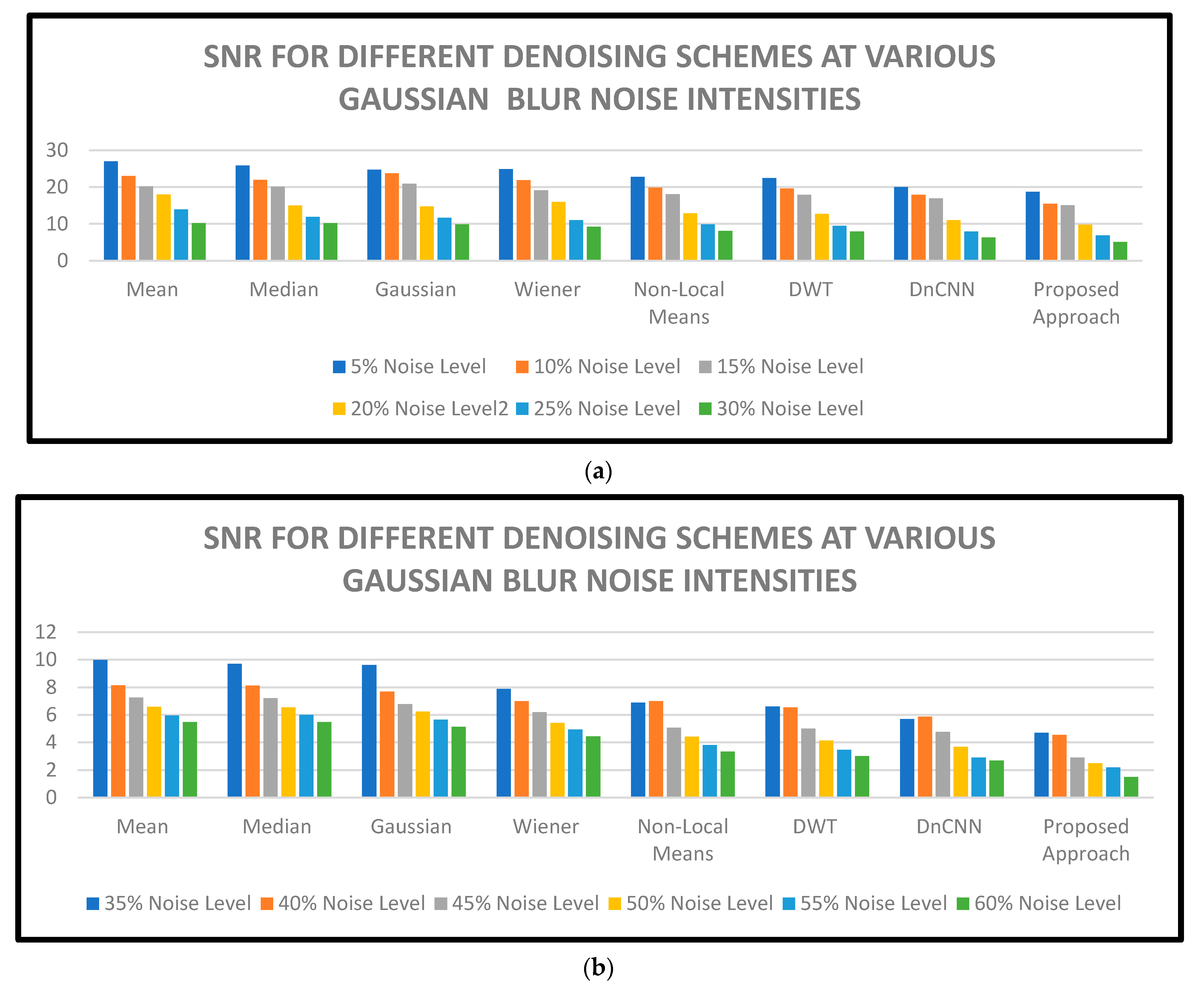
| SNR Values | ||||||
| Denoising Scheme | Gaussian Blur Noise at Different Intensities (%) | |||||
| 5% | 10% | 15% | 20% | 25% | 30% | |
| Non-Local Means [23] | 22.7497 | 19.8691 | 18.0366 | 12.8525 | 9.8674 | 8.0812 |
| Gaussian [24] | 24.7053 | 23.7319 | 20.8656 | 14.7141 | 11.6318 | 9.9032 |
| Median [25] | 25.8455 | 21.9760 | 20.1306 | 15.0174 | 11.8910 | 10.2377 |
| DWT [27] | 22.4563 | 19.6455 | 17.8646 | 12.6789 | 9.4673 | 7.8956 |
| Mean [28] | 26.9982 | 22.9896 | 20.1805 | 18.0253 | 13.9653 | 10.2240 |
| Wiener [42] | 24.8508 | 21.8702 | 19.1477 | 15.9636 | 10.9785 | 9.1923 |
| DnCNN [56] | 20.0456 | 17.8654 | 16.9213 | 11.0486 | 7.9564 | 6.2893 |
| Proposed Approach | 18.6893 | 15.4563 | 15.0895 | 9.7987 | 6.8956 | 5.1124 |
| SNR Values | ||||||
| Denoising Scheme | Gaussian Blur Noise at Different Intensities (%) | |||||
| 35% | 40% | 45% | 50% | 55% | 60% | |
| Non-Local Means [23] | 6.8752 | 6.9932 | 5.0735 | 4.4100 | 3.8214 | 3.3328 |
| Gaussian [24] | 9.6175 | 7.6793 | 6.7695 | 6.2262 | 5.6484 | 5.1261 |
| Median [25] | 9.6986 | 8.1305 | 7.2202 | 6.5345 | 5.9930 | 5.4779 |
| DWT [27] | 6.5986 | 6.5467 | 5.0032 | 4.1264 | 3.4574 | 3.0042 |
| Mean [28] | 9.9898 | 8.1453 | 7.2461 | 6.5730 | 5.9483 | 5.4735 |
| Wiener [42] | 7.8863 | 7.0043 | 6.1846 | 5.4212 | 4.9325 | 4.4439 |
| DnCNN [56] | 5.6845 | 5.8697 | 4.7589 | 3.6895 | 2.8964 | 2.6874 |
| Proposed Approach | 4.6978 | 4.5535 | 2.8975 | 2.4967 | 2.1895 | 1.4984 |
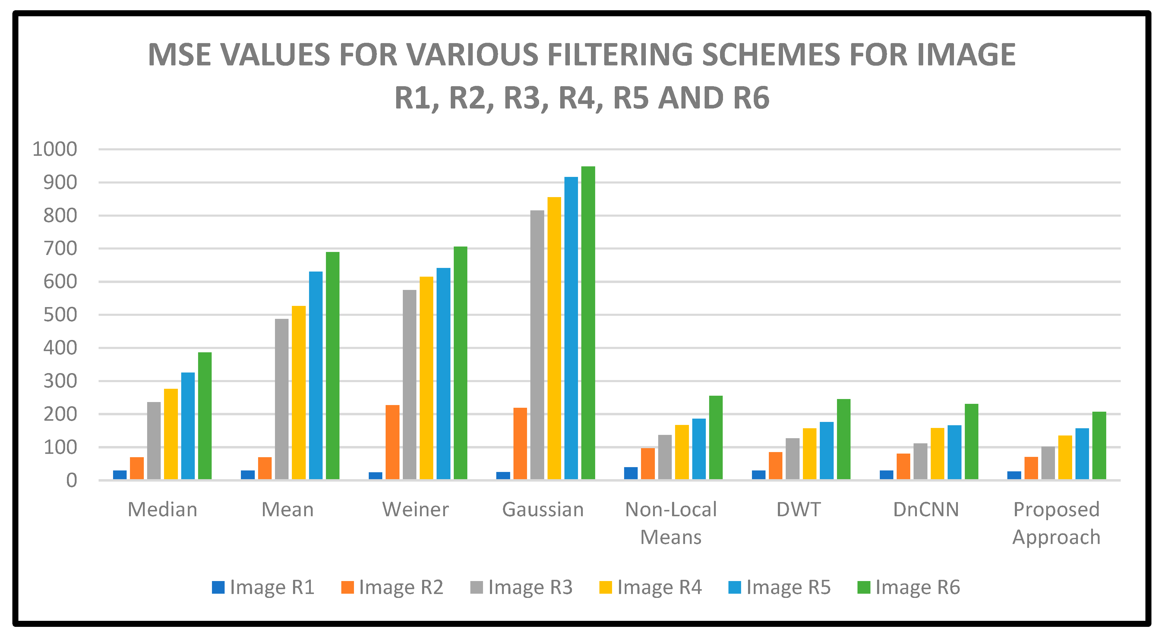
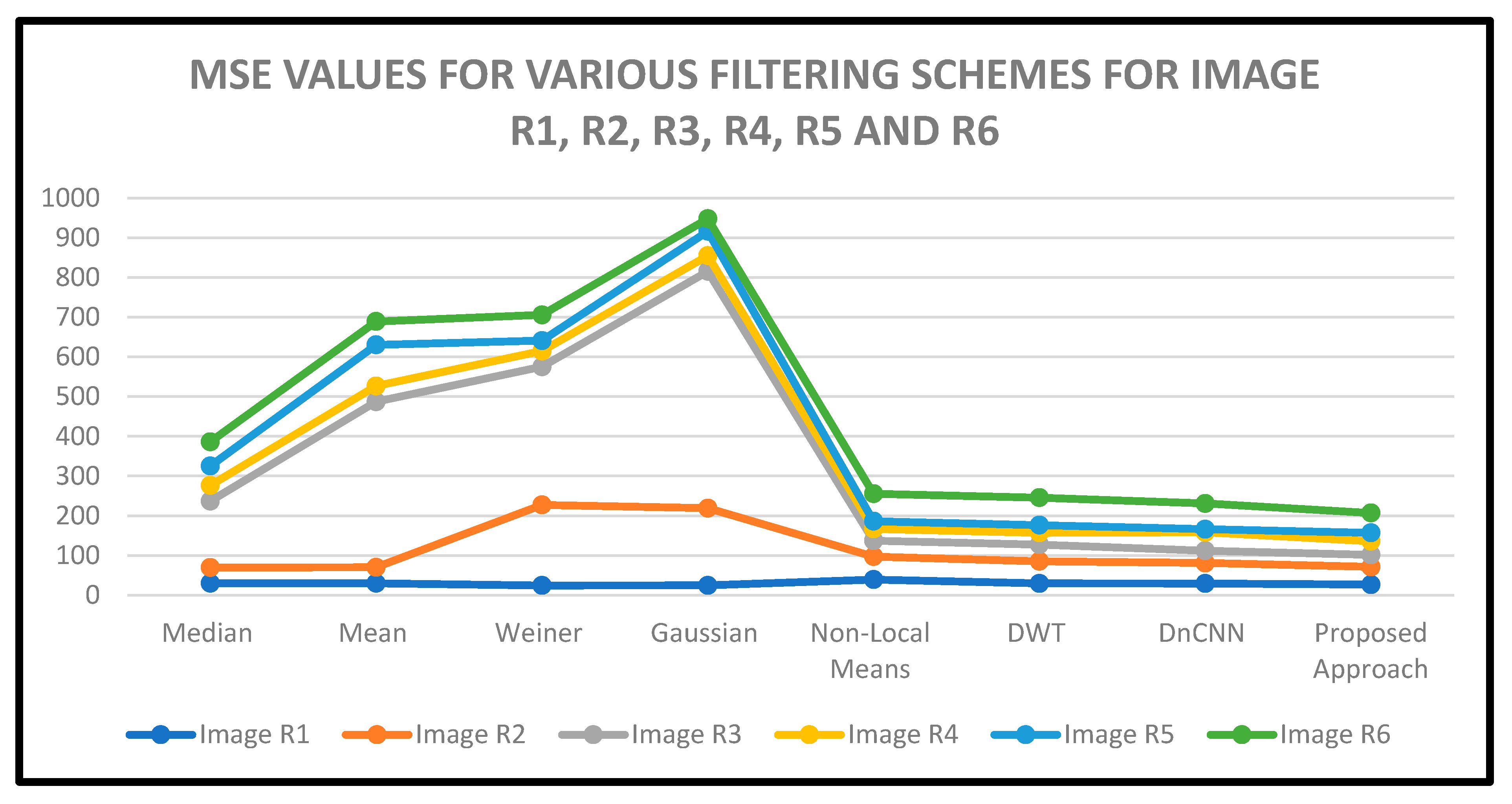
| IMAGE | Median [25] | Mean [28] | Wiener [42] | Gaussian [24] | NLM [23] | DWT [27] | DnCNN [56] | Proposed Approach |
|---|---|---|---|---|---|---|---|---|
| Image R1 | 29.7189 | 29.7290 | 24.5629 | 24.5736 | 39.3783 | 29.3783 | 29.2486 | 26.4634 |
| Image R2 | 69.3731 | 69.9344 | 227.4001 | 218.8388 | 97.0323 | 85.0321 | 80.9547 | 70.9867 |
| Image R3 | 236.6997 | 487.1047 | 575.0933 | 815.4983 | 137.1280 | 127.1280 | 111.8759 | 101.3453 |
| Image R4 | 276.3539 | 526.7589 | 614.7475 | 855.1525 | 166.7822 | 156.7822 | 158.0136 | 135.6523 |
| Image R5 | 325.3523 | 630.4532 | 640.8953 | 916.2461 | 186.0234 | 176.0234 | 165.8954 | 156.8953 |
| Image R6 | 386.2341 | 689.2313 | 705.7646 | 947.9875 | 255.2488 | 245.3478 | 230.8694 | 206.9078 |
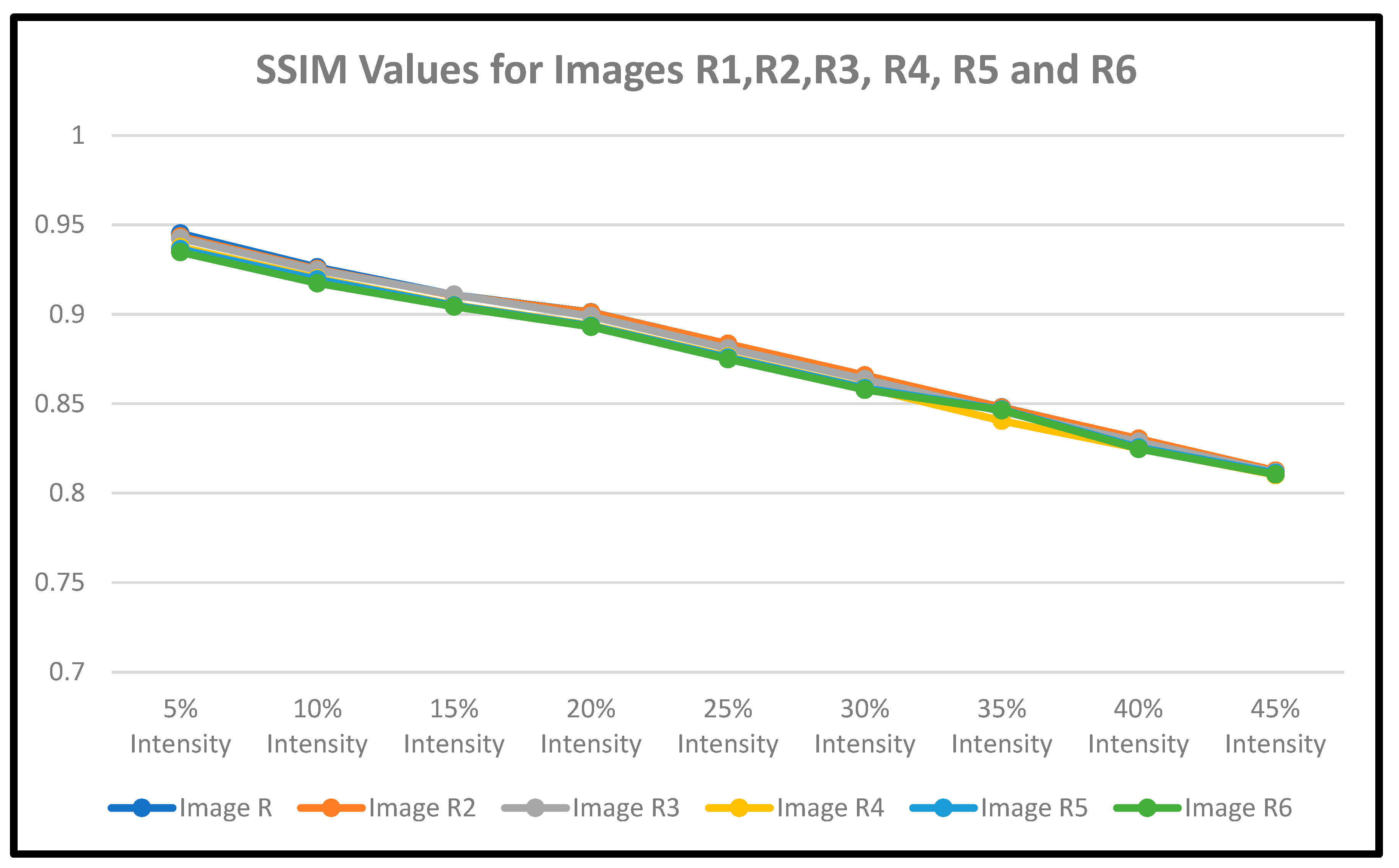
| Noise Density | Image R1 | Image R2 | Image R3 | Image R4 | Image R5 | Image R6 |
|---|---|---|---|---|---|---|
| SSIM Values | ||||||
| 5% | 0.945185 | 0.943385 | 0.942513 | 0.937519 | 0.936408 | 0.934789 |
| 10% | 0.926260 | 0.925201 | 0.924620 | 0.920162 | 0.919456 | 0.917345 |
| 15% | 0.910734 | 0.910573 | 0.910914 | 0.905187 | 0.904893 | 0.904291 |
| 20% | 0.901130 | 0.900996 | 0.898911 | 0.893868 | 0.893466 | 0.892968 |
| 25% | 0.883405 | 0.883405 | 0.880901 | 0.876379 | 0.875789 | 0.874897 |
| 30% | 0.865680 | 0.865809 | 0.863623 | 0.859061 | 0.858735 | 0.857798 |
| 35% | 0.847955 | 0.847882 | 0.845612 | 0.840414 | 0.846746 | 0.846345 |
| 40% | 0.830230 | 0.830382 | 0.828658 | 0.825006 | 0.825534 | 0.824784 |
| 45% | 0.812505 | 0.812528 | 0.811728 | 0.810150 | 0.811231 | 0.810543 |
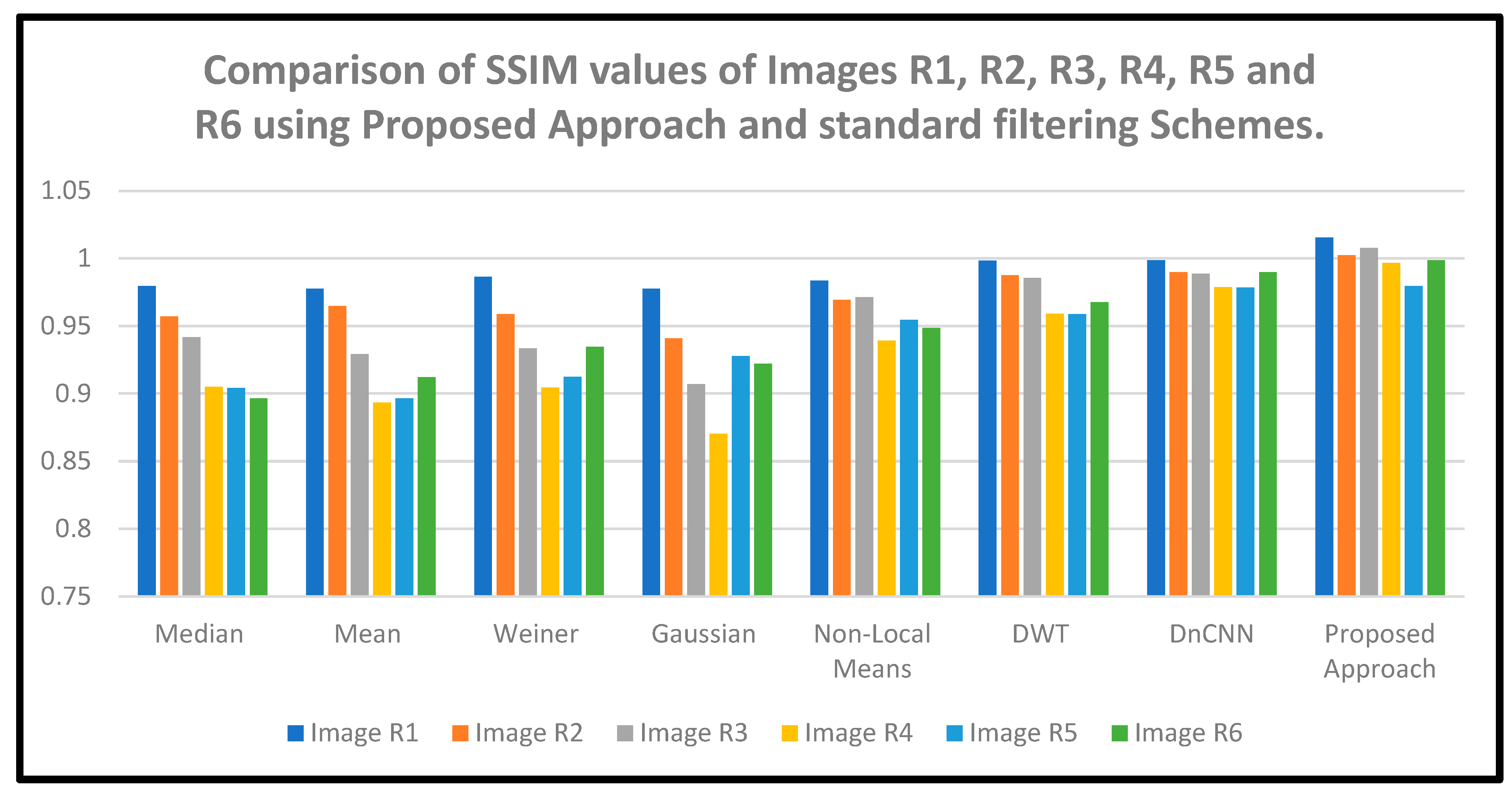
| SSIM Values | ||||||||
|---|---|---|---|---|---|---|---|---|
| CT Images | Median [25] | Mean [28] | Wiener [42] | Gaussian [24] | NLM [23] | DWT [27] | DnCNN [56] | Proposed Approach |
| Image R1 | 0.9796 | 0.9775 | 0.9863 | 0.9774 | 0.9834 | 0.9952 | 0.9987 | 1.000 |
| Image R2 | 0.9570 | 0.9647 | 0.9589 | 0.9408 | 0.9694 | 0.9876 | 0.9899 | 1.000 |
| Image R3 | 0.9418 | 0.9291 | 0.9335 | 0.9071 | 0.9712 | 0.9854 | 0.9887 | 1.0000 |
| Image R4 | 0.9051 | 0.8934 | 0.9045 | 0.8703 | 0.9391 | 0.9591 | 0.9786 | 0.9967 |
| Image R5 | 0.9042 | 0.8963 | 0.9123 | 0.9278 | 0.9545 | 0.9589 | 0.9785 | 0.9796 |
| Image R6 | 0.8964 | 0.9121 | 0.9345 | 0.9221 | 0.9486 | 0.9675 | 0.9897 | 0.9986 |
Disclaimer/Publisher’s Note: The statements, opinions and data contained in all publications are solely those of the individual author(s) and contributor(s) and not of MDPI and/or the editor(s). MDPI and/or the editor(s) disclaim responsibility for any injury to people or property resulting from any ideas, methods, instructions or products referred to in the content. |
© 2023 by the authors. Licensee MDPI, Basel, Switzerland. This article is an open access article distributed under the terms and conditions of the Creative Commons Attribution (CC BY) license (https://creativecommons.org/licenses/by/4.0/).
Share and Cite
Abuya, T.K.; Rimiru, R.M.; Okeyo, G.O. An Image Denoising Technique Using Wavelet-Anisotropic Gaussian Filter-Based Denoising Convolutional Neural Network for CT Images. Appl. Sci. 2023, 13, 12069. https://doi.org/10.3390/app132112069
Abuya TK, Rimiru RM, Okeyo GO. An Image Denoising Technique Using Wavelet-Anisotropic Gaussian Filter-Based Denoising Convolutional Neural Network for CT Images. Applied Sciences. 2023; 13(21):12069. https://doi.org/10.3390/app132112069
Chicago/Turabian StyleAbuya, Teresa Kwamboka, Richard Maina Rimiru, and George Onyango Okeyo. 2023. "An Image Denoising Technique Using Wavelet-Anisotropic Gaussian Filter-Based Denoising Convolutional Neural Network for CT Images" Applied Sciences 13, no. 21: 12069. https://doi.org/10.3390/app132112069