A Novel Method for Multistage Degradation Predicting the Remaining Useful Life of Wind Turbine Generator Bearings Based on Domain Adaptation

Abstract

Predicting the remaining useful life (RUL) of wind turbine generator rolling bearings can effectively prevent damage to the transmission chain and significant economic losses resulting from sudden failures. However, the working conditions of generator bearings are variable, and the collected run-to-failure data combine multiple working conditions, which significantly impacts the accuracy of model predictions. To solve the problem, a local enhancement temporal convolutional network with multistage degenerate distribution matching based on domain adaptation (MDA-LETCN) is proposed, extracting degradation features of wind turbine generator bearings and predicting their remaining service life in composite working conditions. This method first utilizes the local enhancement temporal convolutional network (LETCN) to extract time series features and used the K-means method for unsupervised division of the degradation status of rolling bearings. Secondly, the multistage degradation stage distribution matching (MDSDM) module is proposed to learn domain-invariant temporal features at different stages of bearing degradation under composite working conditions. Finally, the model is transferred to the target bearing using some health data that are easily available from the target bearing to solve the problem of individual differences in the degradation of generator bearings in different wind turbines. Comparative experiments were conducted using actual wind farm data, and the results showed that MDA-LETCN has high prediction accuracy.

1. Introduction

Wind energy, as a renewable and clean energy, has developed rapidly worldwide. Wind turbines (WT) are an important equipment for converting wind energy into electricity. With the gradual increase in operating time, transmission chain failures gradually appear [1]. As one of the important parts of the transmission chain, the rolling bearing is affected by the wind speed and operates under the condition of variable speed for a long time, which is prone to failure, affecting the stability of the WT operation and even leading to casualties [2,3,4]. In addition, the replacement of rolling bearings has a long cycle and high cost. Consequently, monitoring the operational status of WT generator rolling bearings and predicting their remaining useful life (RUL) hold significant importance in preventing escalating maintenance costs and averting catastrophic accidents caused by bearing failures.

WTs are usually equipped with condition monitoring systems (CMS) to monitor the operating status of key components of the transmission chain for a long time and periodically collect vibration signals [5,6]. Because of the long collection time, the full life information can be collected, which provides the possibility for RUL prediction of rolling bearings of WTs.

RUL prediction methods can be broadly categorized into two groups: physical model-based methods [7,8] and data-driven methods [9,10]. Physical model-based requires the development of precise physical models to describe the degradation process of WTs. However, the transmission chain structure of WTs is very complex and the working conditions are changeable, so it is difficult to establish an accurate physical model. Data-driven RUL prediction models have received increasing attention with the rapid development of artificial intelligence [11,12,13]. Xiang et al. [14] proposed a novel multihierarchy network based on multiordered neurons and realized RUL prediction for gearbox and bearings. Ni et al. [15] developed a new health indicator (HI) for RUL prediction of bearings using a Bayesian optimization gated recurrent unit network (GRU). Yang et al. [16] added two attention gates to GRU to construct a bidirectional structural prediction bearing RUL. However, all the methods used in the above research can be classified as the improvement of recurrent neural network (RNN), whose training mode is based on recurrent recursive structure and can only process one sample at a time, which leads to the shortcoming of long-term dependence and affects RUL prediction effect.

Temporal convolutional neural network (TCN) represents an enhancement of convolutional neural network (CNN). By extending causal convolution, temporal features of historical data can be extracted, while also possessing the advantages of CNN’s expandable acceptance domain and parallel computing. Compared with RNN structures such as GRU, TCN not only avoids information leakage from the future to the present but also improves prediction efficiency and has excellent prediction ability [17,18]. Wang et al. [19] proposed a competitive TCN that enhances feature extraction capabilities and improves the accuracy of the model’s RUL prediction for rolling bearings. Peng et al. [20] proposed a novel multiscale temporal convolutional transformer that takes into account both long-term and short-term potential degradation features of bearings, effectively capturing long-term dependency coupling while improving local feature learning ability. The superiority of this proposed method was empirically validated using experimental datasets.

In the above studies, the effectiveness was verified using the laboratory accelerated bearing life dataset. However, the laboratory accelerated life experiments were all conducted under a single working condition, and the data structure was good. During the actual operation of WTs, the speed of the generator bearings varies with the wind speed. However, the CMS of WTs collects vibration signals regularly, so it is difficult to collect the run-to-failure data at a certain fixed speed. This time variation in speed will affect the degradation rate of the bearing and increase the amplitude fluctuation of working parameters in condition monitoring, which is a great challenge to the RUL prediction of practical engineering WT generator bearings [21]. Domain adaptive (DA) is an important branch of transfer learning. DA maps the features of different working conditions into a new feature space with the same distribution as much as possible, which is an effective solution for predicting bearing RUL under different working conditions [22,23,24]. Miao et al. [25] used selective convolutional RNN to extract features from vibration signals and proposed a co-operative domain alignment method to learn domain-invariant features. Hu et al. [26] proposed a deep feature disentanglement transfer learning network to reduce the distribution differences of features under different working conditions. Rathore et al. [27] used multi-kernel maximum mean discrepancy (MMD) to achieve DA under different working conditions.

The methods mentioned above primarily involved transferring models from one working condition to another. However, the full life data of WT generator bearings is a combination of multiple working conditions. It is not realistic to establish a model for each working condition. More importantly, it is impossible to separate the run-to-failure data with equal time intervals and roughly the same working conditions for training the model. Therefore, designing an RUL prediction method for WT generator bearings under composite working conditions is of great significance for practical engineering applications. So, a local enhancement time convolutional model with multistage degenerate distribution matching based on domain adaptation (MDA-LETCN) for WT generator bearing RUL prediction is proposed in this paper. This method proposes local enhancement TCN to learn the temporal features of generator bearing data and uses the K-means for unsupervised and divides the bearing degradation state into three stages: healthy state, slight degradation, and severe degradation state. Secondly, a multistage degradation stage distribution matching (MDSDM) is set up, and MDSDM aligns the distribution of features at different degradation stages, promoting the model to learn the degradation laws at different stages under composite working conditions. Finally, part of the health data of the target bearing is used to reduce the degradation of individual differences in the generator bearings of different WTs by DA, and the model is transferred to adapt to the target bearing. Experimental verification was conducted using actual WT life cycle data from a wind farm in Shandong and compared with advanced methods. The results showed that the prediction accuracy of the proposed method is higher. The novelties of this work are as follows:

(1)

RUL prediction methods for WT generator bearings under composite working conditions are proposed, which utilizes TCN with local enhanced residual module to extract temporal features and unsupervised K-means to partition the degradation status of generator bearings.

(2)

Aiming at the problem that the prediction accuracy of the full life data of WT generator bearings is affected by the cross-fusion working conditions, the MDSDM module is proposed, which can reduce the influence of composite working conditions on the model and help the model learn the degradation features independent of working conditions.

(3)

In view of the different degradation trends of WT generator bearings caused by working conditions, fault types, and other reasons, the DA module is added to the model to improve the prediction accuracy of the model in the target domain bearings.

The rest of this paper is structured as follows. Section 2 introduces WT generator bearing data, data preprocessing, and the construction method of HI. Section 3 presents the details of the MDA-LETCN. Section 4 introduces the prediction results of MDA-LETCN and compares them with advanced methods in six tasks. Section 5 makes some conclusions.

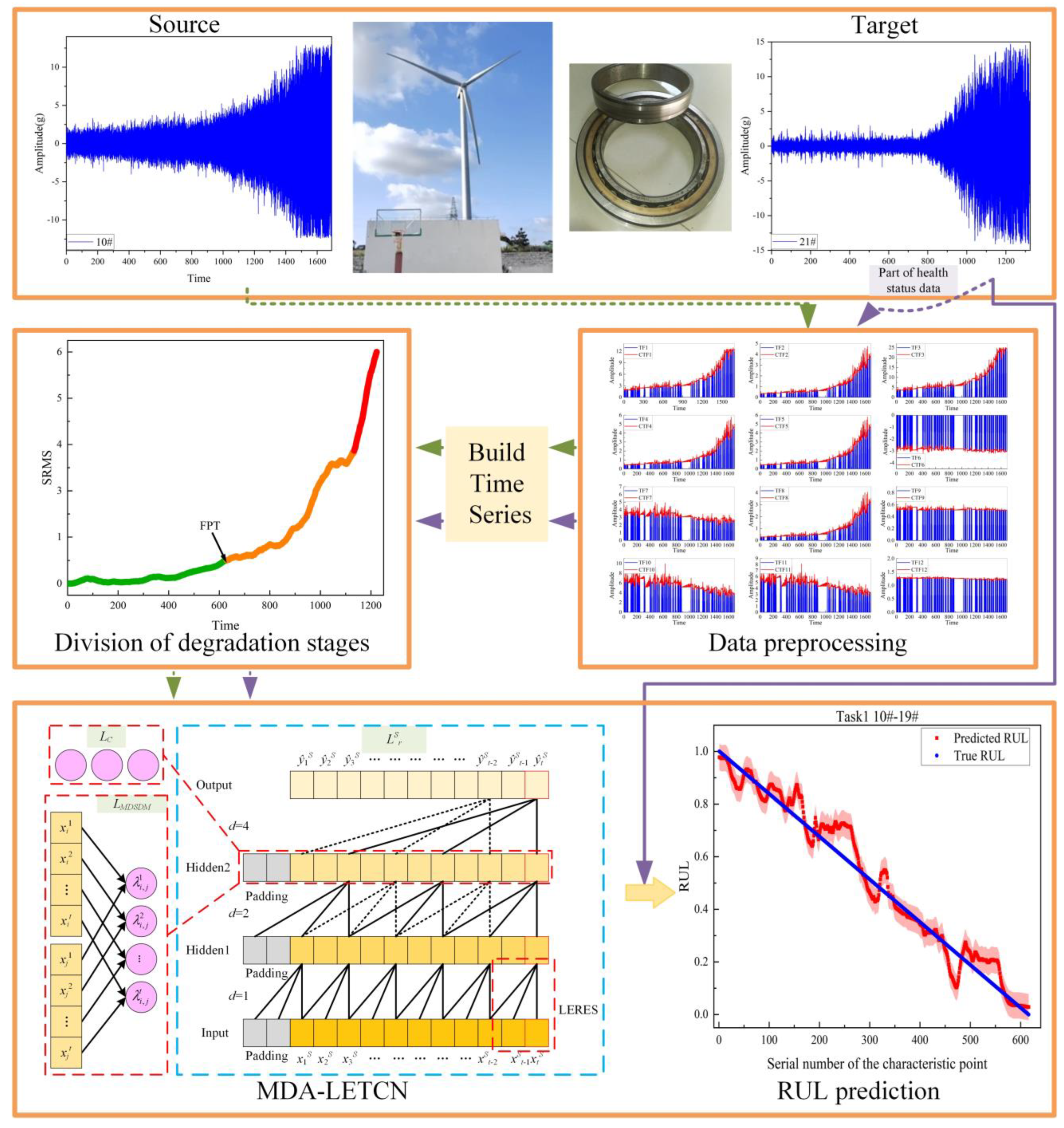
2. Description of the Datasets and Data Preprocessing

In this section, the WT generator bearing data used is introduced, and the methods for data preprocessing and health indicator construction are also introduced.

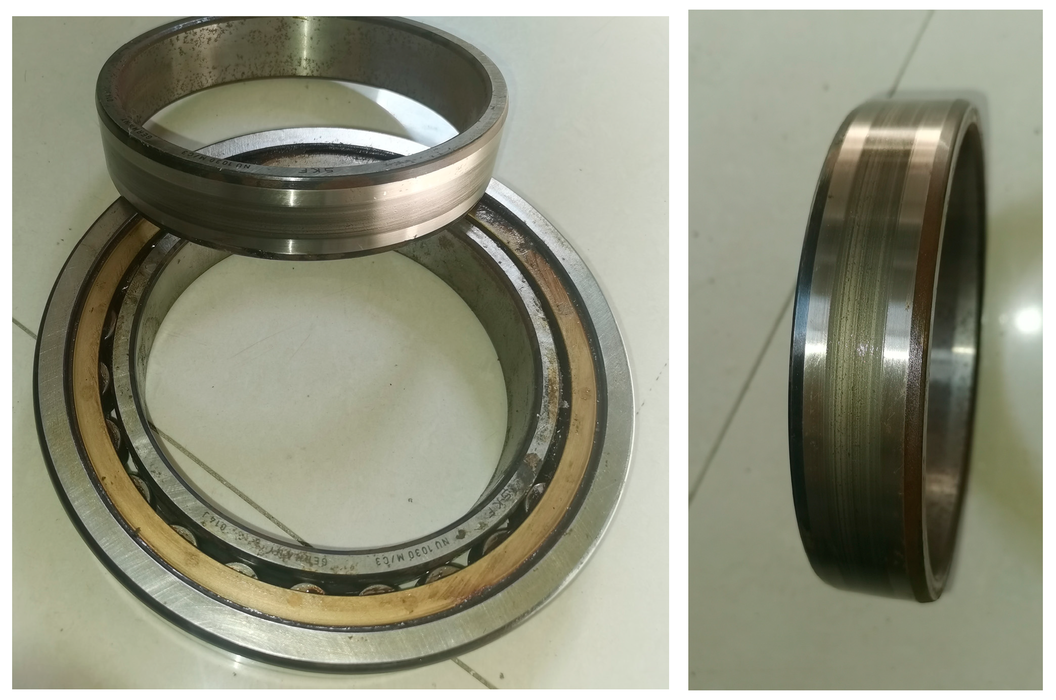
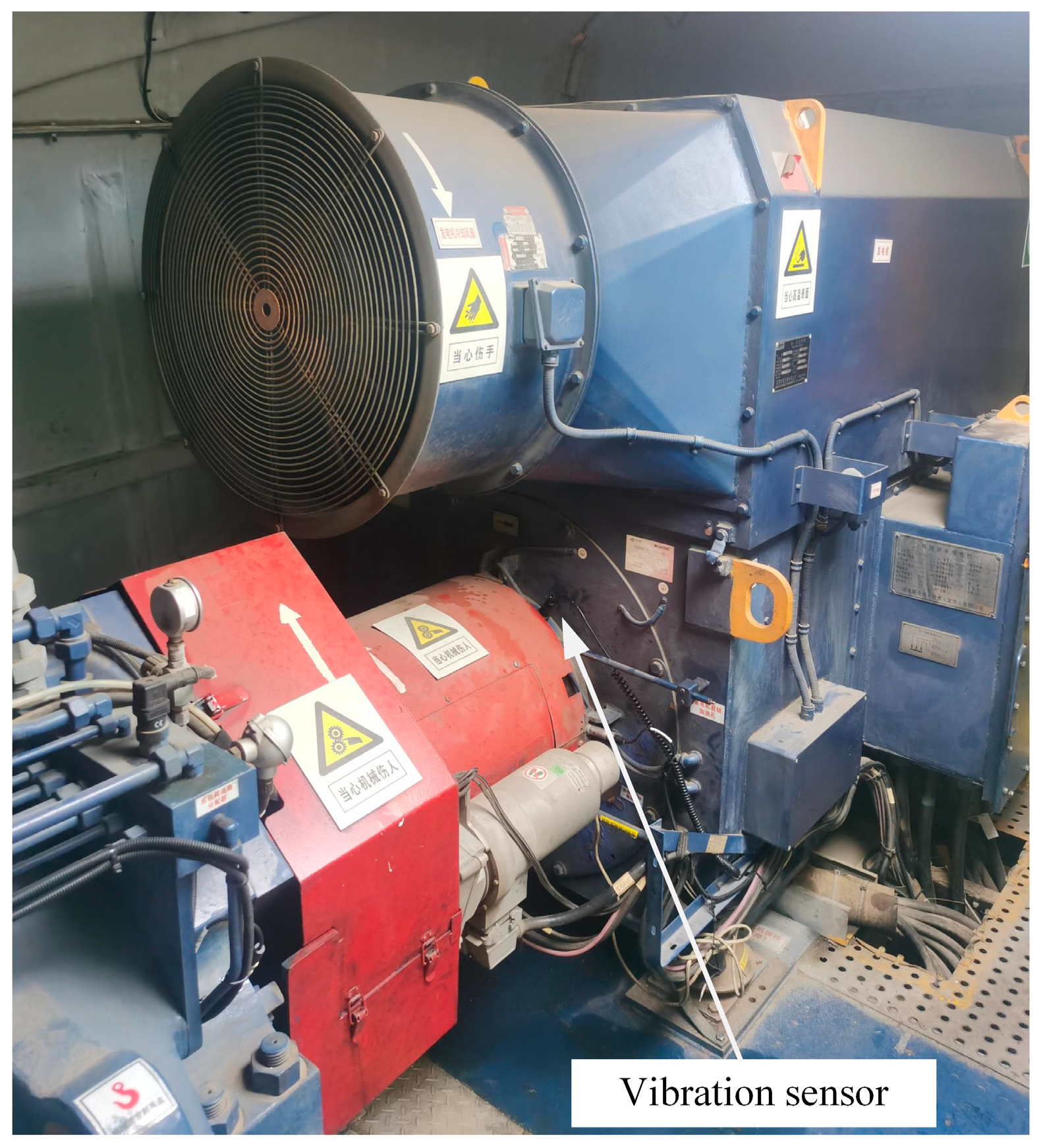
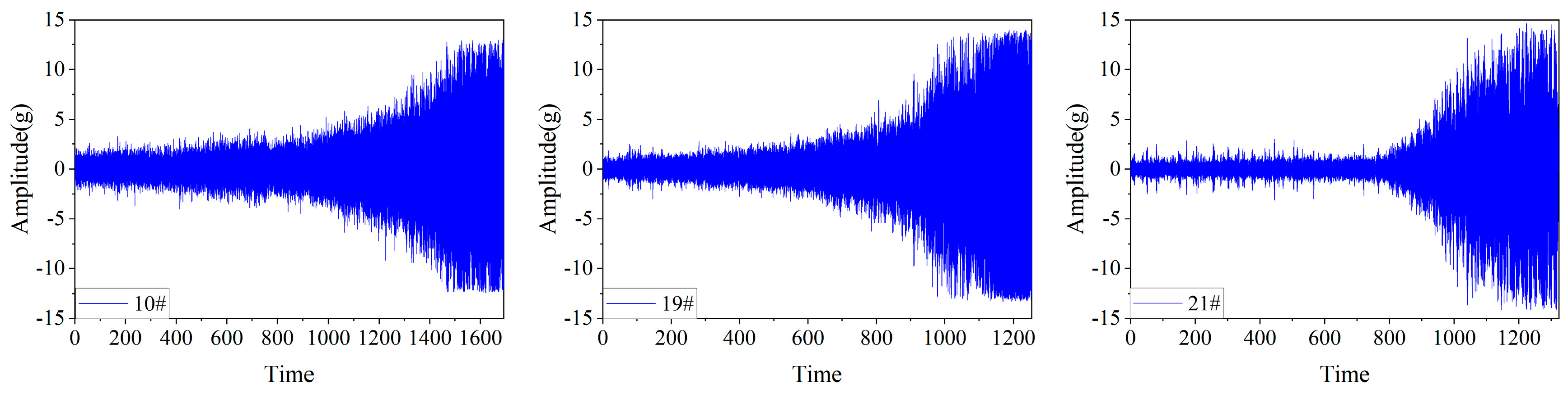
2.1. Description of the Datasets

The lifetime vibration data of WT generator bearings in this paper were obtained from 23 WTs with an installed capacity of 1.5 MW, located within a wind farm in Shandong, China. The generator bearings in this wind farm were of the NU1030M model. Since July 2017, the generator bearings of the three WTs 10#, 19#, and 21# have been collected, which were degraded from healthy operation to severe failure then were replaced by the wind farm. After replacement, the faulty bearings were disassembled, as shown in Figure 1. In this paper, the criterion for bearing failure is based on the replacement of bearings within the wind farm. This CMS records a vibration signal every hour, with a single sampling time of 1.28 s and a sampling frequency of 12,800 Hz; the data collection system is shown in Figure 2. Figure 3 is the time-domain signals of the entire life of the three WTs from operation in July 2017 to bearing replacement. To represent the degradation trends of WT bearings, time-domain features (TF) are extracted based on vibration acceleration [28,29,30], as shown in

Table 1. Time domain degradation feature.

Features	Equations	Features	Equations
Peak	$T{F}_1=\max \left|x_t\right|$	Kurtosis	$T{F}_7=\frac{1}{T\cdot T{F}_5^4}{\displaystyle \sum _{t=1}^T{\left(x_t-T{F}_2\right)}^4}$
Mean absolute value	$T{F}_2=\frac{1}{T}{\displaystyle \sum _{t=1}^T\left|x_t\right|}$	Square root amplitude	$T{F}_8={\left(\frac{1}{T}{\displaystyle \sum _{t=1}^T\sqrt{\left|x_t\right|}}\right)}^2$
Peak to peak	$T{F}_3=\max \left(x_t\right)-\min \left(x_t\right)$	Crest factor	$T{F}_9=\frac{T{F}_1}{T{F}_4}$
Root mean square(RMS)	$T{F}_4=\sqrt{\frac{1}{T}{\displaystyle \sum _{t=1}^T{x}_t^2}}$	Clearance factor	$T{F}_{10}=\frac{T{F}_1}{T{F}_8}$
Standard deviation	$T{F}_5=\sqrt{\frac{1}{T-1}{\displaystyle \sum _{t=1}^T{\left(x_t-T{F}_2\right)}^2}}$	Impulse factor	$T{F}_{11}=\frac{T{F}_1}{T{F}_2}$
Skewness	$T{F}_6=\frac{1}{T\cdot T{F}_5^3}{\displaystyle \sum _{t=1}^T{\left(x_t-T{F}_2\right)}^3}$	Shape factor	$T{F}_{12}=\frac{T{F}_4}{T{F}_2}$

.

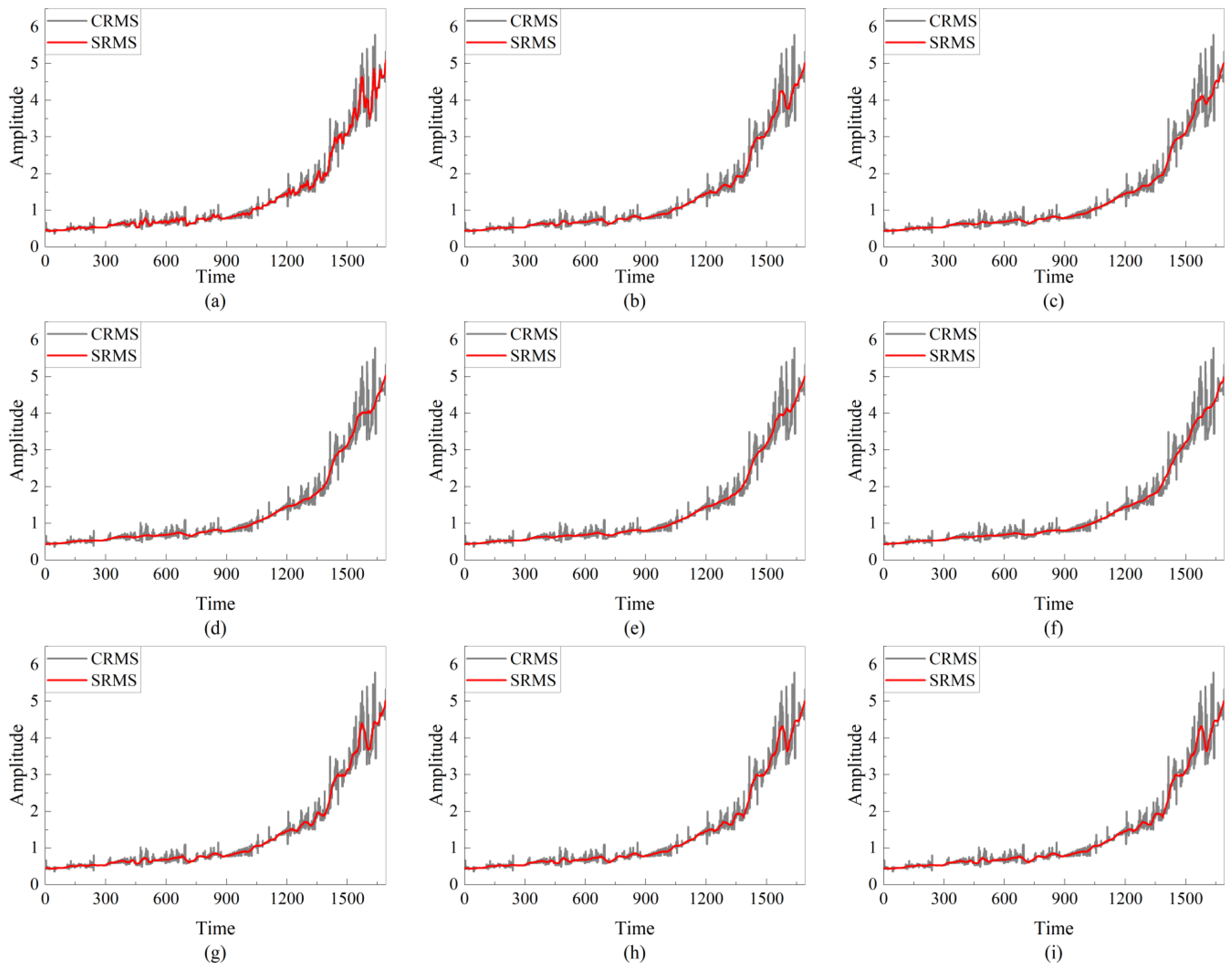
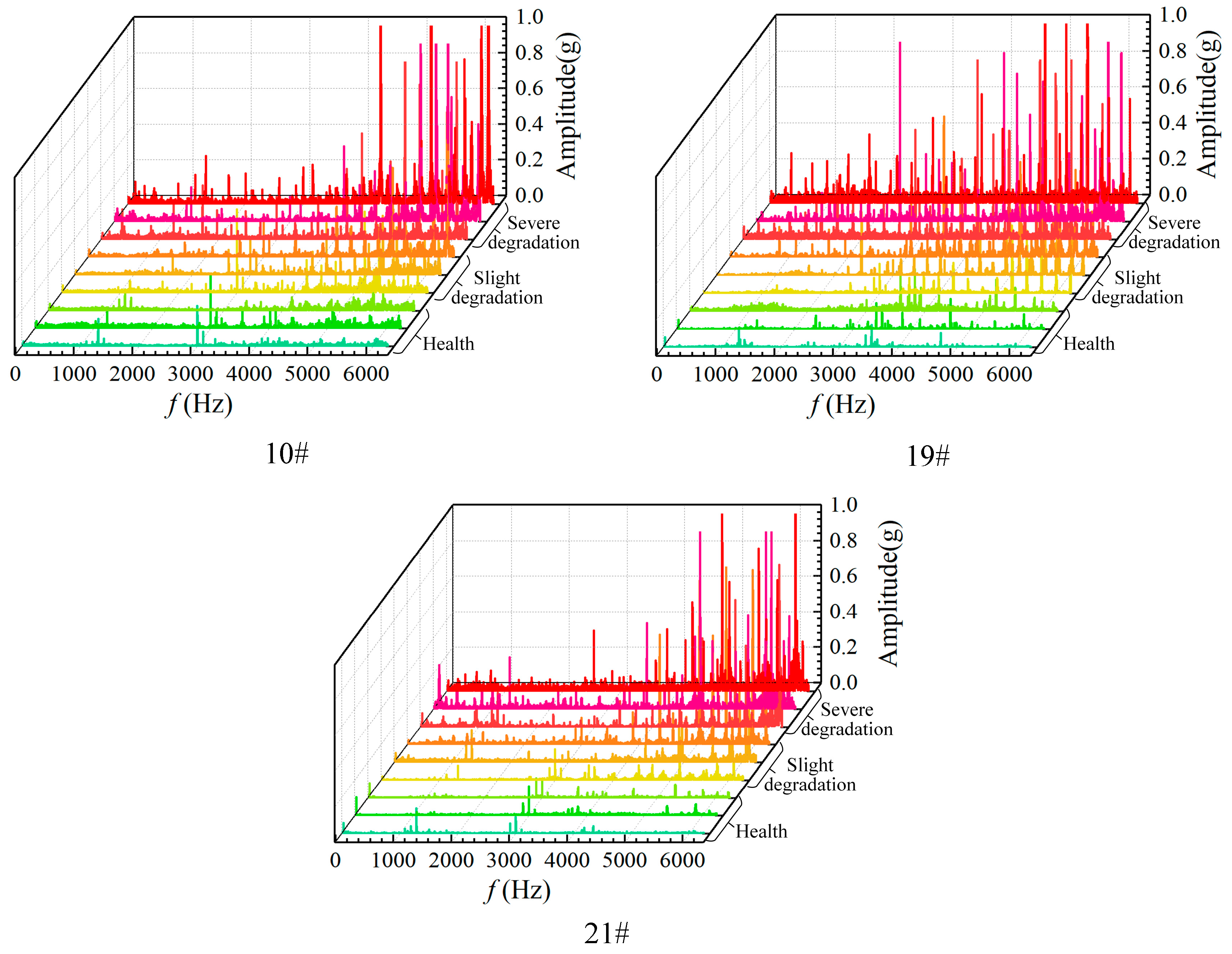
2.2. Data Preprocessing

Firstly, WTs are powered by wind, so the speed of the generator vibration signals collected by CMS at regular intervals is not constant. It is evident that fluctuations in speed will inevitably impact the amplitude, peak value, and other features of the vibration signal. This will cause great difficulties for the RUL predicting of generator bearings. To solve this problem, firstly, considering that WTs do not generate electricity when the speed falls below 1000 RPM or above 1800 RPM, data within this range should be filtered and deleted. Secondly, when the wind direction changes sharply in a short period of time, the yaw system of the WT automatically starts, which may lead to unstable operation of the generator, and the data under such speed are excluded. Finally, if the limited speed range is too small, the available data will be greatly reduced. Based on the above principles, this paper selected the vibration signal with the speed of 1100 RPM–1600 RPM to extract features.

Secondly, when RUL is predicting, the acquired signals need to meet an equal interval. Considering the actual operating conditions, the degradation process is slow, so it is assumed that the degradation state of the bearing is the same in one day so that a vibration signal meeting the speed range can be selected in the 24 data a day to represent the running state of the day. The predicted time interval is one day.

Finally, in the actual operation of WTs, there are inevitable shutdowns for maintenance, which will lead to the loss of vibration signals from generator bearings. Additionally, due to the uncertainty of wind speed, it is challenging to ensure that the speed of all 24 vibration signals collected in a day falls within the previously mentioned speed range. Therefore, it is necessary to complete the missing data. This paper utilizes the interpolation method for completion operations. Figure 4 shows the CTF image of RUL features after the original 12 TFs and complete time domain features (CTF) of the WT No. 10#.

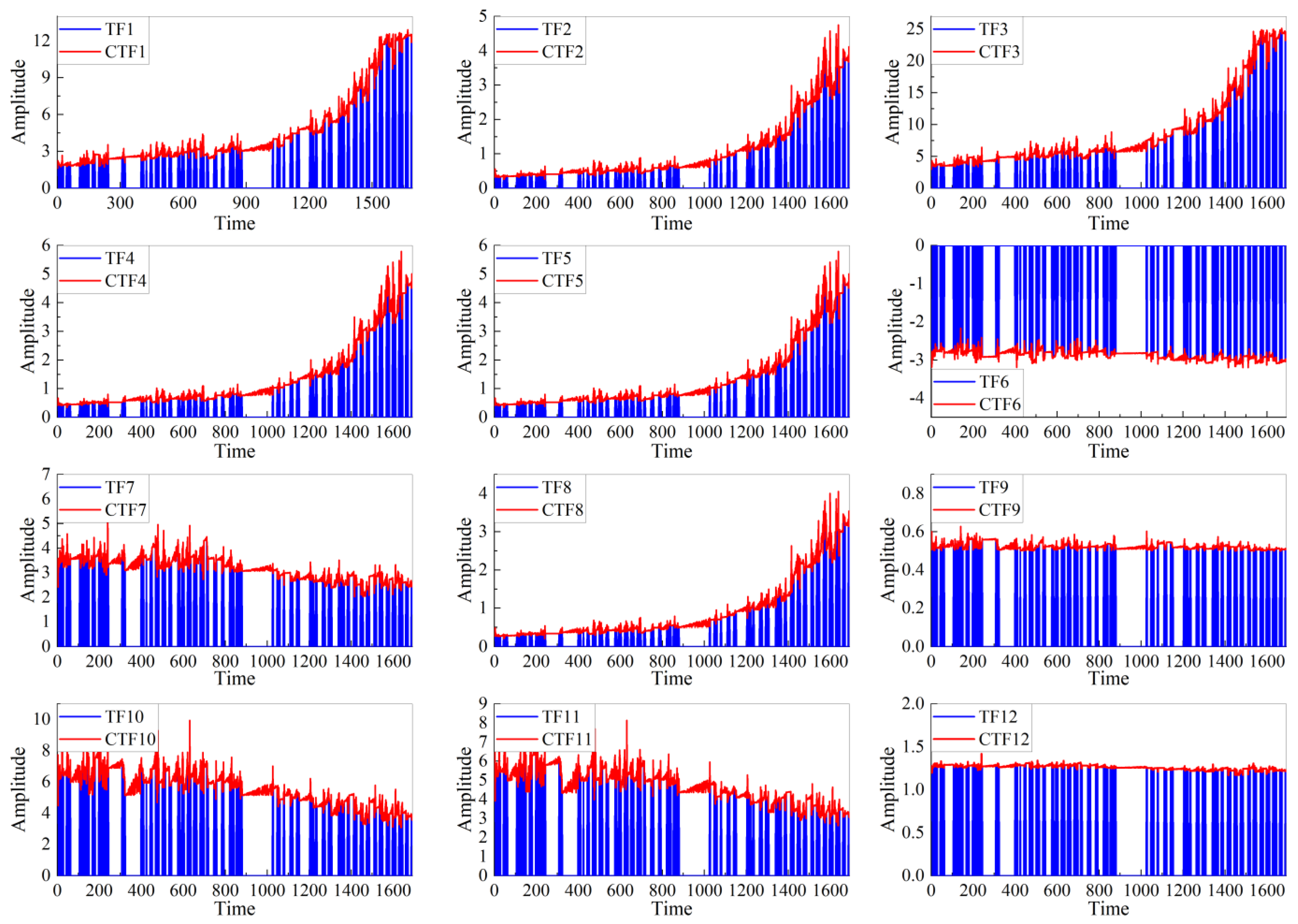
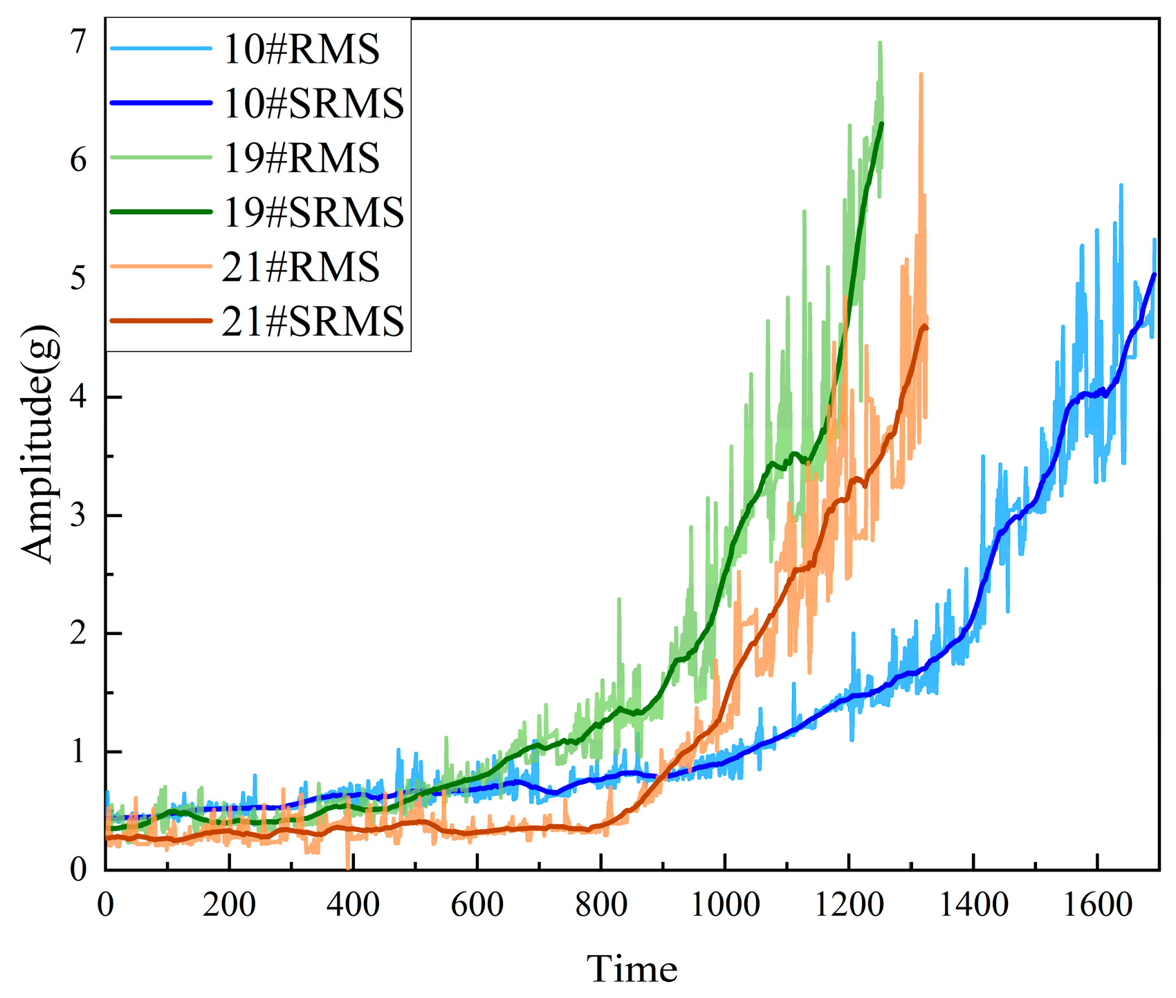
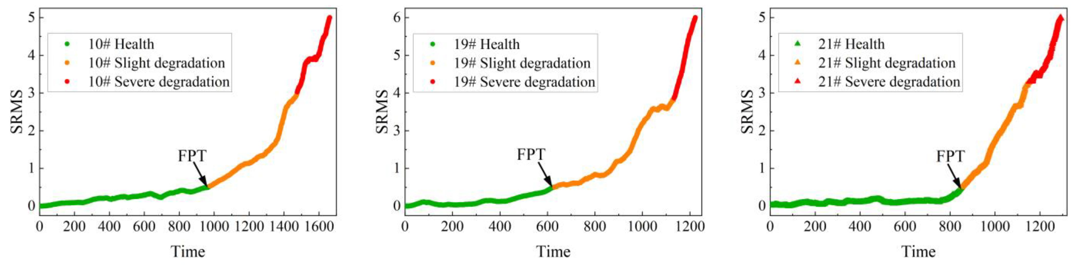
2.3. HI Construction

HI is very important in RUL prediction of bearings, and RMS can reflect the degradation status of bearings and is commonly used as an indicator for dividing bearing status as HI. However, the generator bearing speed in the run-to-failure data in the actual wind farm is not fixed, and there must be random fluctuations in the RMS calculated under composite working conditions, which is not a typical phenomenon of bearing degradation and will seriously affect the prediction effect. To reduce the random fluctuations in RMS, this paper uses the Savitzky–Golay filter (SG) to smooth RMS and obtains SRMS as the HI and the other 11 features as model inputs [31,32].

SG is a smoothing technique that relies on interval polynomial fitting, with the ability to filter out random fluctuations in the data without changing the shape and trend of the original data. The key to SG smoothing is to use a (k − 1)-order polynomial to fit points centered on the selected data point within a window length of 2m + 1, and the polynomial formula is:

$$y=a_0+a_{1}x+a_2{x}^2+\cdots +a_{k-1}{x}^{k-1}$$

(1)

Then, for 2m + 1 points in the window, there are 2m + 1 equations:

$$\left(\begin{array}{l}{y}_{-m}\\ y_{1-m}\\ ⋮\\ y_m\end{array}\right)=\left(\begin{array}{cccc}1& x_{-m}& \cdots & {\left(x_{-m}\right)}^{k-1}\\ 1& x_{1-m}& \cdots & {\left(x_{1-m}\right)}^{k-1}\\ ⋮& ⋮& \ddots & ⋮\\ 1& x_m& \cdots & {\left(x_m\right)}^{k-1}\end{array}\right)+\left(\begin{array}{l}{e}_{-m}\\ e_{1-m}\\ ⋮\\ e_m\end{array}\right)$$

(2)

Using matrix form, it can be represented as:

$$Y=AX+E$$

(3)

where Y is the fitting vector, A is the coefficient matrix, X is the independent variable matrix, and E is the residual. The above equation can usually be solved by using the least square method.

$$\overline{A}={\left(X^{T}X\right)}^{-1}{X}^{T}Y$$

(4)

$$\overline{Y}=X\overline{A}=X{\left(X^{T}X\right)}^{-1}{X}^{T}Y$$

(5)

The window slides in chronological order until all data points are fitted, resulting in a smoothed-curve SRMS.

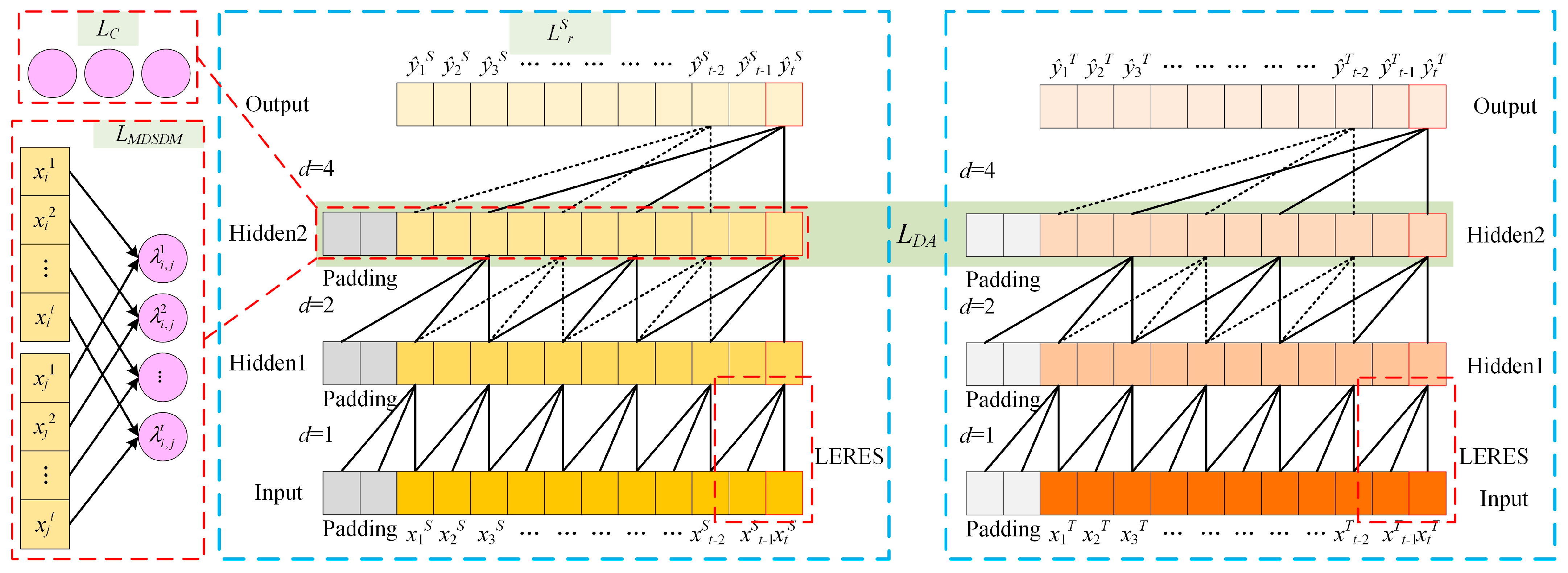
3. The Proposed New Method MDA-LETCN

Figure 5 shows the network structure of MDA-LETCN. MDA-LETCN is composed of a temporal features extraction module, a degradation state division module, an MDSDM, a DA module, and a regression module. The temporal feature extraction module consists of a TCN with locally enhanced residuals (LERES), which is employed to extract temporal features. The degraded state division module utilizes K-means for the unsupervised division of degraded states based on the temporal features extracted by LETCN. The MDSDM module is used to match the distribution differences of different degradation stages, learn domain-invariant degradation features, and eliminate the problem of unsatisfactory prediction accuracy caused by feature amplitude fluctuations in the composite working conditions of WT generator bearings. The DA module is used to reduce the distribution differences between source and target domain and improve the prediction accuracy in the target domain. Finally, the final prediction result is obtained by the regression module.

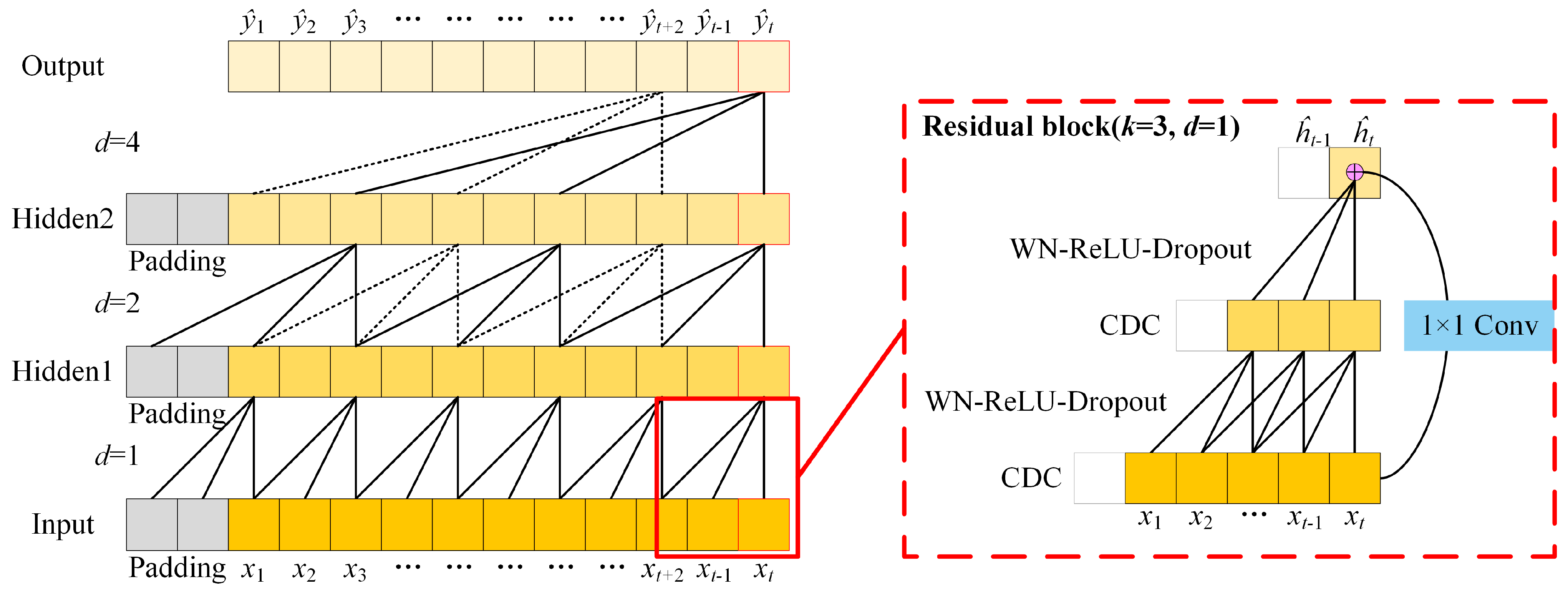
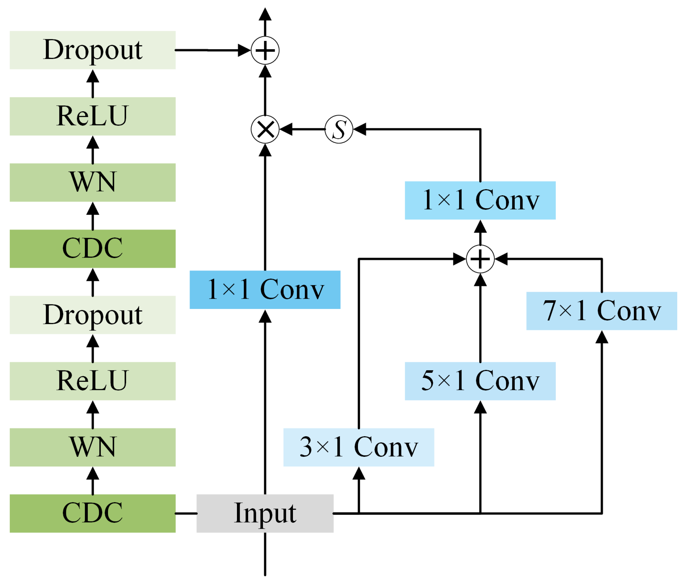
3.1. Temporal Feature Extraction Module

In this paper, the temporal convolution structure is used to extract the time information of generator bearings’ degradation process. TCN is a network structure based on CNN, which is composed of causal convolution, dilated convolution, and residual modules, which can learn the temporal features of time series in parallel and avoid leakage.

• Causal dilated convolutions

Figure 5 shows the structure of the causal dilated convolutions (CDC) network, which is composed of causal convolution and dilated convolution. Causal convolution learns temporal features based on current and historical information to predict the value at the next moment, that is, using $\left\{x_1,x_2,\cdots ,x_t\right\}$ to predict the value of x_t+1. The formula is:

$$p(x)={\displaystyle \prod _{t=1}^{T}p}\left\{x_{t+1}|x_1,x_2,\cdots ,x_t\right\}$$

(6)

If only the causal convolution learning temporal feature is relied on, the model needs to build deeper and have a larger convolution kernel size to increase the receptive field to achieve the ideal effect. This results in increased model complexity. To solve this problem, the dilated convolution and the combination with causal convolution can greatly reduce the complexity of the model. The receptive field for CDC with expansion rate d is:

$$k^l=\left(d-1\right)\cdot \left(k_c^l-1\right)+k_c^l$$

(7)

where $k_c^l$ is the convolution kernel of l-layer causal convolution and $k_{}^l$ is the receptive field size of l-layer CDC. The final output value of the model depends on the coverage of the model. In order to ensure the low complexity and large receptive field of the model, with each additional layer, the expansion rate of the current layer will increase at the rate of b, and the receptive field width of each layer can also be expressed as:

$$w=1+{\displaystyle \sum _{l=0}^{L-1}(k-1)\cdot b^l}=1+(k-1)\frac{b^l-1}{b-1}$$

(8)

where the dilated rate $d=b^l$ and l represents the number of layers in the model. When inputting layers, l = 0 and k is the size of the convolutional kernel.

It is worth noting that dilated convolution can cause voids in the receptive field. To prevent information loss, a residual structure as shown in Figure 6 is added to TCN. This residual structure includes two layers of CDC. After each CDC, the weights are normalized using weight normalization and the ReLU function is used as the activation function to prevent model overfitting. Finally, the result obtained after 1 × 1 convolution is added to the results of the two CDC, and the output is:

$$out=\mathrm{ReLU}(x+f(x))$$

(9)

where f(.) represents two CDC-WN-ReLU-Dropout operation transformations. This residual structure not only ensures the integrity of information but also extracts sufficiently long time series features.

TCN utilizes CDC and residual structure to extract long-term temporal features of time series but ignores the importance of local features. In this paper, MDA-LETCN adds a local enhancement module to the residual module of TCN, which pays attention to local features while extracting long-term historical information and improves the prediction accuracy of model RUL.

LETCN adds a local information enhancement module in the residual module to improve the original 1 × 1 convolution to the structure shown in Figure 7. First, the features of input signal x are extracted by the convolution operation with convolution kernels of 3, 5, and 7, respectively.

$$o_i=con{v}_i(x),i=1,2,3$$

(10)

Then, the three output signals are spliced according to dimension:

$$o=\mathrm{concat}(o_1+o_2+o_3)$$

(11)

Next, the features of the three channels are compressed by 1 × 1 convolution kernel and integrated by activation function to obtain the weight of each time point:

$$w=\mathrm{Sigmoid}(con{v}_{1\times 1}(o))$$

(12)

Finally, the output of the LERES is:

$$out=\mathrm{ReLU}(w\ast o+f(x))$$

(13)

The model uses mean square error (MSE) as the loss function, i.e.:

$$L_r=\mathrm{MSE}(y_i,{\widehat{y}}_i)=\frac{1}{N}{\displaystyle \sum _{i=1}^N{\left(y_i-{\widehat{y}}_i\right)}^2}$$

(14)

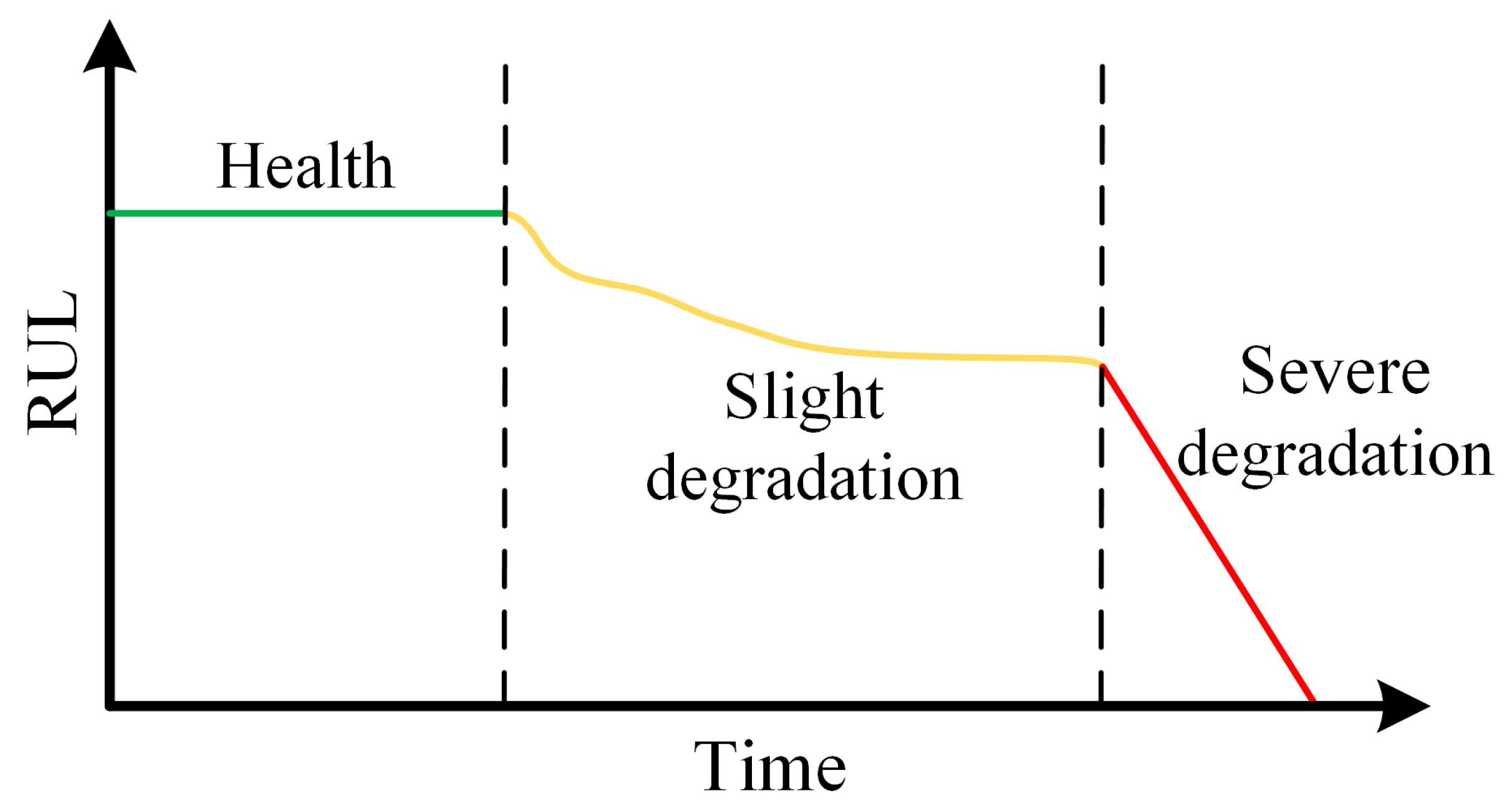
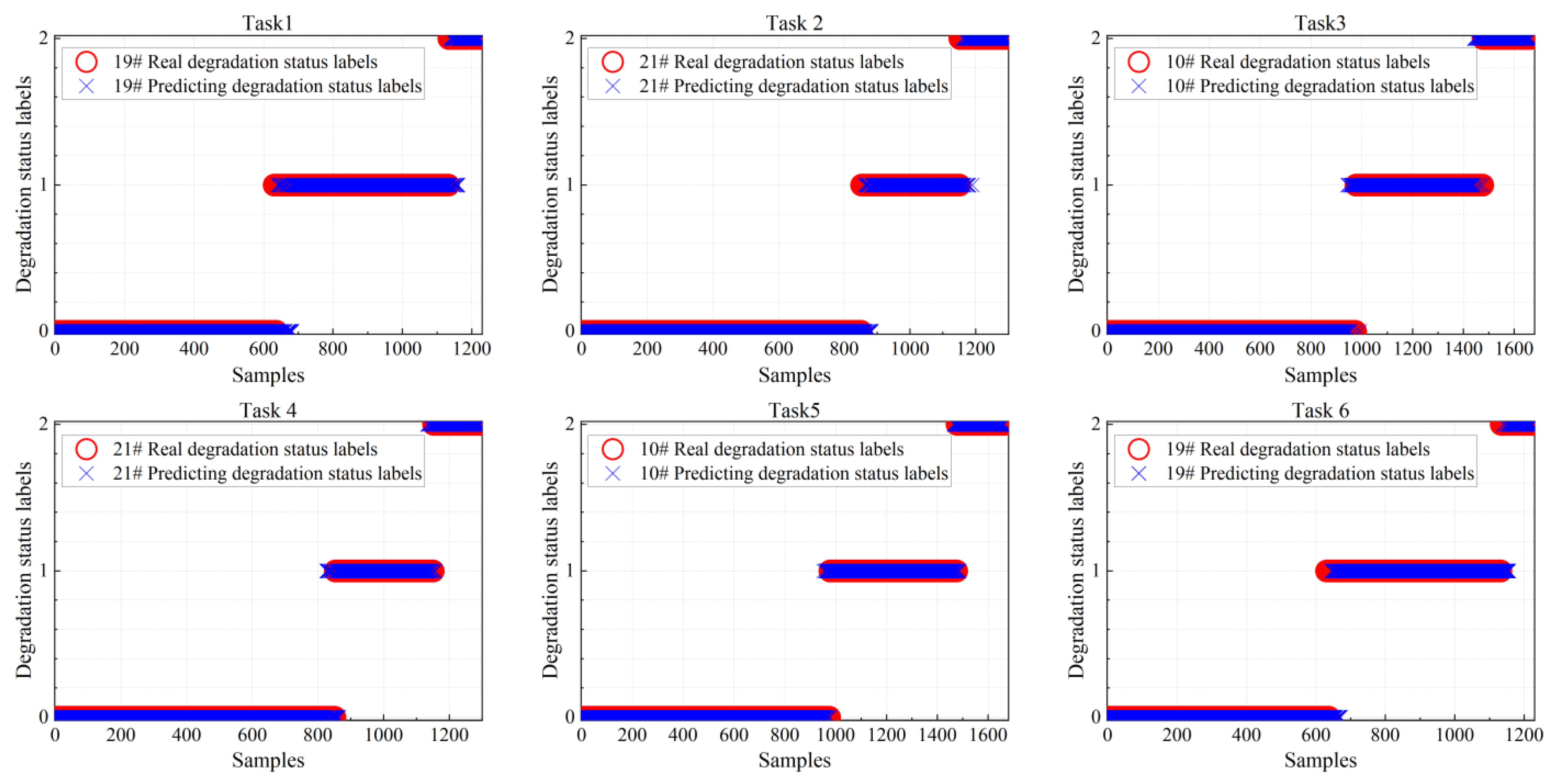
3.2. Multistage Degradation State Division

In the existing studies, the degradation state of rolling bearings is divided either manually based on expert experience or by setting thresholds for HI, but the two have a large degree of subjective awareness in the process of division, which cannot be promoted. In addition, the life data of WT generator bearings are in a composite working condition, and fluctuating speed will lead to an increase in the feature amplitude. This also makes the selection of thresholds extremely difficult. To solve the above problems, this section sets a clustering module in the network, and unsupervised divides the bearing degradation state while learning the bearing degradation features.

Considering the actual operating status of WTs during the operation and maintenance process of wind farms, this paper divides the operating status of generator bearings into three stages: health, slight degradation, and severe degradation, as shown in Figure 8.

In order to reduce the impact of feature amplitude fluctuations caused by composite working conditions on the division of degraded states and improve the accuracy of the model in classifying degraded states, the clustering loss is added during the model training process:

$$L_C=\frac{1}{2}{\displaystyle \sum _{i=1}^N{\Vert x_i-c_{x_i}\Vert }_2^2}$$

(15)

where $c_{x_i}$ is the cluster center of $x_i$, and cluster loss will make the model learn more effective features for degenerate-state recognition based on learning time series.

3.3. Multistage Degradation Stage Distribution Matching (MDSDM)

There is a significant distribution difference between the three degradation stages of TW generator bearings during operation from health-state degradation to bearing replacement. If the model has high prediction accuracy in each degradation stage, the prediction model must learn the domain-invariant time dependence in different degradation stages of generator bearings. However, the signals of generator bearings collected by the CMS are under composite working conditions, which will seriously affect learning the domain-invariant features. In this paper, an MDSDM module is proposed. By reducing the distribution difference between different degradation stages, the model can learn the domain-invariant degradation features between the multi-degradation stages and improve the prediction RUL accuracy of the model for generator bearings. For the same type of bearing, the internal physical degradation mechanism will not be affected by the composite working condition. So, MDSDM can effectively extract the degradation features of the bearing under the composite working condition. For the feature sets D_i and D_j of different degradation stages, the loss of MDSDM is:

$$L_{MDSDM}(D_i,D_j)={\displaystyle \sum _{t=1}^T{\lambda }_{i,j}^{t}d(x_i^t,x_j^t)}$$

(16)

where $x_i^l\in D_i$ and $x_j^l\in D_j$ are the t eigenvalues of the i and j stages, respectively, ${\lambda }_{i,j}^t$ is the importance of distribution, and d is the distance function, defined as the cosine similarity function in this paper. In this paper, the importance of dynamic evaluation of temporal features is observed, that is, dynamic update parameter ${\lambda }_{i,j}^t$. Firstly, the source domain is used to take $L_r+\alpha L_C$ as the loss pretraining model, enabling the model to better learn the temporal features in the bearing degradation process. In the training process, the initial weight is set to the same value, that is, ${\lambda }_{i,j}^t=1/T,t=1,2,\cdots ,T$. Then, with the increase in iterations during formal training, if the distribution distance of n iterations is greater than n − 1 iterations, the distribution difference becomes larger, so the weight is increased to better reduce the distribution difference. Otherwise, the weights remain the same. The updating process of distributed importance is as follows:

$${\lambda }_{i,j}^{n+1,t}=\{\begin{array}{l}{\lambda }_{i,j}^{n,t}\times \left(1+\sigma \left({\lambda }_{i,j}^{n,t}-{\lambda }_{i,j}^{n-1,t}\right)\right) {\lambda }_{i,j}^{n,t}-{\lambda }_{i,j}^{n-1,t}\ge \epsilon \\ {\lambda }_{i,j}^{n,t} \hspace{1em}\hspace{1em}\hspace{1em}otherwise\end{array}$$

(17)

where ${\lambda }_{i,j}^{n,l}$ represents the distribution difference of the tth feature between stage i and stage j during the nth iteration process, $\sigma \left(x\right)=1/\left(1+e^{-x}\right)$, $\epsilon \to 0$. From Equation (17), it can be seen that $\sigma \left(x\right)>0$; when ${\lambda }_{i,j}^{n,t}-{\lambda }_{i,j}^{n-1,t}\ge \epsilon$, ${\lambda }_{i,j}^{n+1,t}$ will increase. Then, the final weight values are obtained by regularizing the ${\lambda }_{i,j}^{n+1,t}={\lambda }_{i,j}^{n+1,t}/\left({\displaystyle \sum _{t=1}^T{\lambda }_{i,j}^{n+1,t}}\right)$.

3.4. Domain Adaptation

In the same wind farm, the bearing models of the WT generators are the same, and their degradation process is the same theoretically. However, the location of each WT and the degradation reasons for bearings are different from the others due to factors such as assembly and lubrication. So, the degradation state of each WT is different. After learning the degradation features from one WT generator bearing, the model is directly applied to the generator bearing of another, and the prediction effect will be worse.

Before the prediction of a new WT, we can easily obtain the vibration data of the health state of the WT generator bearings. In this paper, the lifetime data used in training are added as the source domain, the predicted bearing is taken as the target domain, and part of the normal data of the target is taken as the training set. The model is transferred to the model available in the target domain through DA between the source domain and the health state of the target domain. Therefore, the model adds DA losses:

$$\begin{array}{l}{L}_{DA}\left(D_1^S,D_1^T\right)=\mathrm{MMD}\left(D_1^S,D_1^T\right)\\ =\Vert \frac{1}{{\left|D_1^S\right|}^2}{\displaystyle \sum _{i=1}^{\left|D_1^S\right|}{\displaystyle \sum _{j=1}^{\left|D_1^S\right|}k\left(x_i^s,x_j^s\right)+}}\frac{1}{{\left|D_1^T\right|}^2}{\displaystyle \sum _{i=1}^{\left|D_1^T\right|}{\displaystyle \sum _{j=1}^{\left|D_1^T\right|}k\left(x_i^t,x_j^t\right)}-\frac{1}{\left|D_1^S\right|}\frac{1}{\left|D_1^T\right|}{\displaystyle \sum _{i=1}^{\left|D_1^S\right|}{\displaystyle \sum _{j=1}^{\left|D_1^T\right|}k\left(x_i^s,x_j^t\right)}}}\Vert \end{array}$$

(18)

where $x_i^s\in D_1^S$ and $x_i^t\in D_1^T$ represent the health status data in the source and target domain, respectively, MMD(.) represents MMD function, and k( , ) represents the kernel function.

In this paper, the degradation state of WT generator bearings is divided into three stages and the distribution between each two stages is aligned. Therefore, it is necessary to match (3 × 2)/2 = 3 times; then, the final loss function is:

$$L=L_r+\alpha L_C+\frac{1}{3}\beta {\displaystyle \sum _{i,j}^{i\ne j}{L}_{MDSDM}\left(D_i,D_i,\lambda \right)}+\gamma L_{DA}\left(D_1^S,D_1^T\right)$$

(19)

where $\alpha$, $\beta$, and $\gamma$ are hyperparameters and $L_r^t$ is the regression loss of the training set.

3.5. RUL Prediction

As per Section 3.2, the degradation status of the generator bearings is categorized into three stages: healthy, slight degradation, and severe degradation. In the process of predicting RUL, since there is no degradation in the healthy data, it is not meaningful to predict the RUL of generator bearings in a healthy state. Therefore, in this paper, the first time point within the mild degradation stage is determined as the starting time of bearing degradation, denoted as the first predicted time (FPT), and RUL prediction for the bearings commences from this time point. The degradation labels for the data can be represented as:

$$y_{RUL}^s=\frac{n_s-i}{n_s-\mathrm{FPT}}$$

(20)

where n is the number of data in the source domain; when $y_{RUL}^{}=1$, the generator bearing just runs to FPT; then, the model begins to predict RUL; when $y_{RUL}^{}>1$, the bearing is in a healthy state and, when $y_{RUL}^{}<1$, this indicates that the bearing is degraded.

This paper designs an RUL prediction model based on actual WT generator bearings’ run-to-failure data collected from a wind farm in Shandong. The training process is as follows:

Step 1: The collected vibration signals are filtered according to the date and bearing speed; then, TFs are extracted from filtered data and the missing data are completed. Next, the SG filter is used to smooth the RMS to obtain the SRMS. The source domain is $D^S=\left({\mathit{x}}_1^s,{\mathit{x}}_2^s,\cdots ,{\mathit{x}}_{n_s}^s\right)$ and n_s is the number of source domain. The target domain is $D^T=\left({\mathit{x}}_1^t,{\mathit{x}}_2^t,\cdots ,{\mathit{x}}_{n_t^{\prime }}^t\right)$, $n_t^{\prime }$ is the number of health-state data that the target domain participates in training, and ${\mathit{x}}_n^s$ and ${\mathit{x}}_n^t$ both contain 11 features. D^S and D^T together form the training set, with the remaining samples from the target domain used as the test set.

Step 2: The TFs of bearing vibration signals are constructed as time series. The data of T continuous TFs points are intercepted as a time series.

$$\left[\begin{array}{cccc}{\mathit{x}}_1& {\mathit{x}}_2& \cdots & {\mathit{x}}_T\\ {\mathit{x}}_2& {\mathit{x}}_3& \cdots & {\mathit{x}}_{T+1}\\ ⋮& ⋮& \ddots & ⋮\\ {\mathit{x}}_{N-T}& {\mathit{x}}_{N-T+1}& \cdots & {\mathit{x}}_N\end{array}\right]=\left[\begin{array}{c}{\mathit{d}}_1\\ {\mathit{d}}_2\\ ⋮\\ {\mathit{d}}_{N-T}\end{array}\right]$$

(21)

Step 3: Using source domain time series samples, with $L_r+\alpha L_C$ as the loss function and SRMS as the data label pretraining model, the objective is to learn the degradation features of source domain data and the segmentation of degradation stages. Based on the classification of the degradation status of the source domain bearing data, the FPT for the source domain bearings is determined, and then the RUL labels for the source domain bearings are calculated using Equation (20).

Step 4: Equation (19) was used as the loss function to train MDA-LETCN. Based on the source domain data in the training set, the LETCN module was used to learn the time characteristics of bearing degradation and the MDSDM module was used to reduce the difference in feature distribution of each degradation stage based on the division results of the bearing degradation state by the pretraining model so as to learn the domain-invariant degradation characteristics of bearings. For the target domain data in the training set, which only contains health status data, the DA module is used to align the health status feature distribution in the source domain and the target domain so as to migrate the model to the adaptive target bearing.

Step 5: Using the test set test model results, once the FTP of the target bearing is identified by the model, RUL prediction for the target bearing is started.

Figure 9 shows the diagnostic process of MDA-LETCN.

4. Case Studies

In this paper, the whole-life data of three WT generator bearings collected by a wind farm in Shandong are used for experiments. Data details and data preprocessing are described in Section 2. Six transfer tasks, as shown in

Table 2. Transfer learning tasks.

Task	Source	Target
Task1	10#	19#
Task2	10#	21#
Task3	19#	10#
Task4	19#	21#
Task5	21#	10#
Task6	21#	19#

, are constructed to test and validate the effectiveness of MDA-LETCN. The first 300 healthy samples were selected in the target domain to participate in model training.

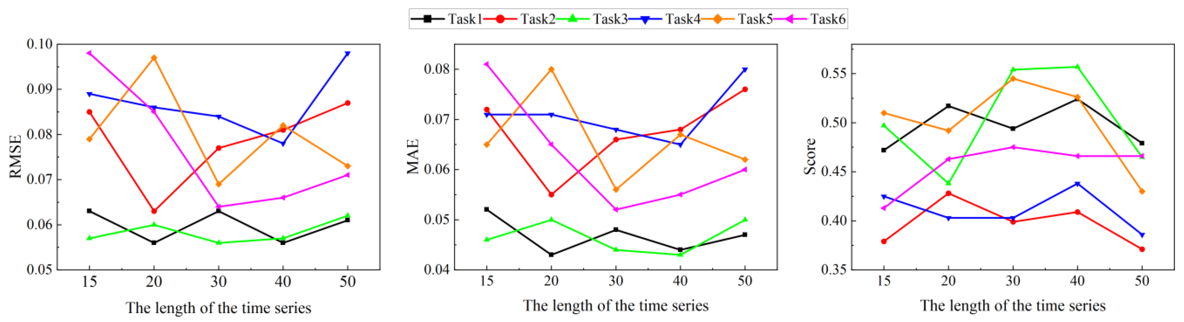
4.1. Parameter Settings

In the calculation of HI, there are two parameters m and k in SG filtering. Figure 10 shows the SRMS curve of the 10 # WT when the two parameters take different values. It can be seen that the selection of these two parameters will directly affect the filtering effect of SG. When k = 2, the larger the m, the better the smoothing effect. At a fixed m value, the higher the k value, the worse the smoothing effect. After comprehensive consideration, this paper selects m = 30 and k = 2. Figure 11 shows the SRMS curve of the three WTs after SG filtering. It can be seen that SRMS retains the degradation trend of WT bearings based on smooth curves.

The MDA-LETCN proposed in this paper needs to cover all time series, with four residual modules set, each with a convolutional kernel size of 3 and channel of 32. $\alpha$ = 0.005, $\beta$ = 0.001, and the learning rate is 0.005.

To verify the effectiveness of MDA-LETCN in predicting RUL, root mean square error (RMSE), mean absolute error (MAE), and score were used as evaluation indicators.

$$\mathrm{RMSE}=\sqrt{\frac{{\displaystyle \sum _{i=1}^N\left(y_i-{\widehat{y}}_i\right)}}{N}}$$

(22)

$$\mathrm{MAE}=\frac{1}{N}{\displaystyle \sum _{i=1}^N\left|y_i-{\widehat{y}}_i\right|}$$

(23)

$$Score=\frac{1}{n}{\displaystyle \sum _{i=1}^n{A}_i}$$

(24)

where:

$$A_i=\{\begin{array}{l}{e}^{-\ln \left(0.5\right)\cdot \left(E{r}_i/5\right)} if E{r}_i\le 0\\ e^{\ln \left(0.5\right)\cdot \left(E{r}_i/20\right)} if E{r}_i>0\end{array}$$

(25)

$$E{r}_i=\frac{y_i-{\widehat{y}}_i}{y_i}\cdot 100$$

(26)

where $y_i$ is the actual RUL, ${\widehat{y}}_i$ is the predicted RUL, and N is the number of data points participating in the test.

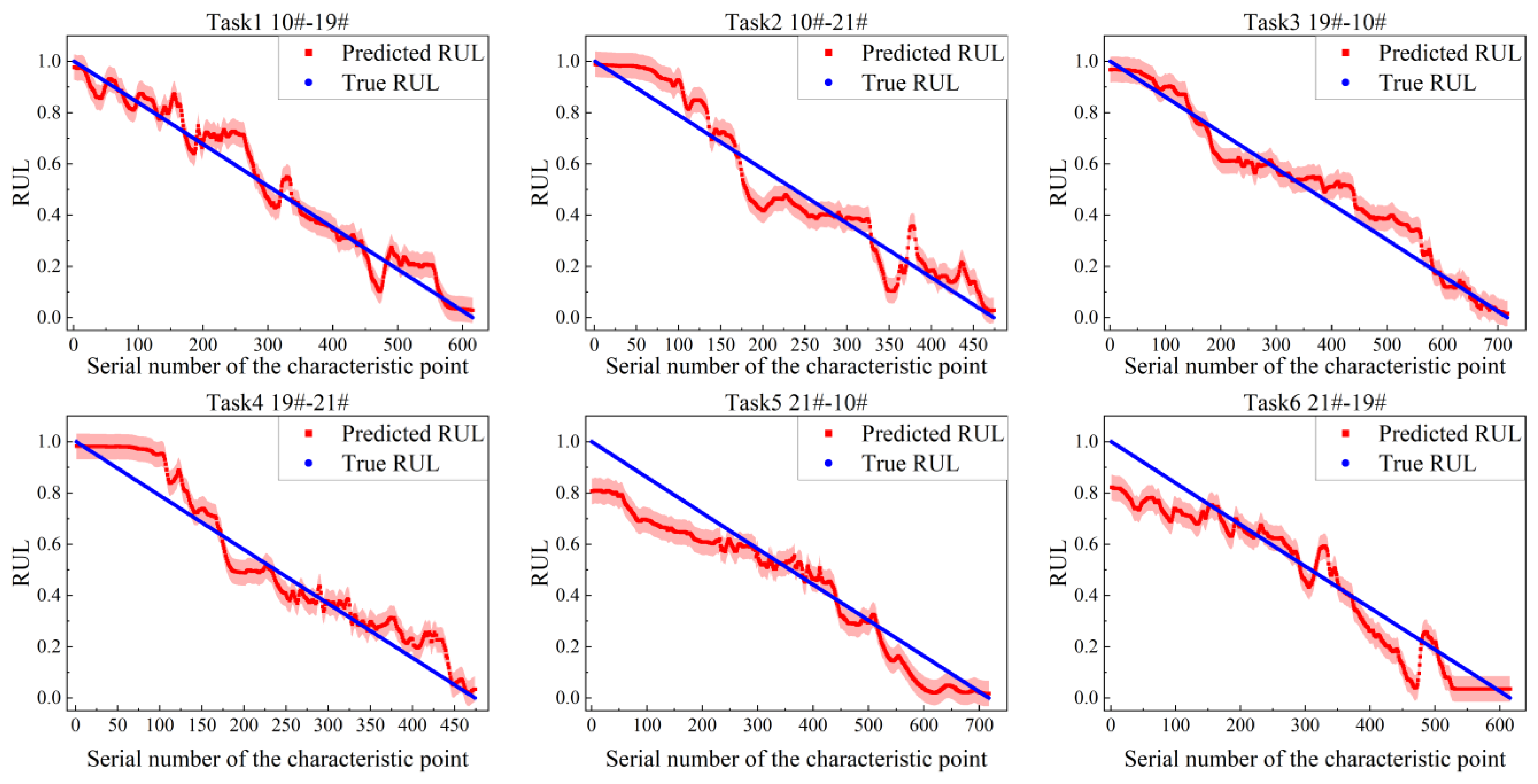
4.2. Results of Degradation State Divided and Prediction RUL

Figure 12 shows the division results of degraded states when the generator bearings of three WT generators are, respectively, used as training datasets. It can be seen that there are differences in the degradation trends of the three WTs but, before a significant degradation trend occurs, all three WTs maintain a healthy state for a long time. This part of the data contains less degradation information, so the point that is initially classified as slightly degraded is chosen as the FPT.

Figure 13 shows the state division of MDA-LETCN for the target domain among six transfer tasks. It can be seen that MDA-LETCN can still accurately classify the degradation status of bearings in the target domain. Although there are a few advanced or delayed points between the two states, the degradation process of bearings is a continuous and slowly changing time series process, and there will be no sudden changes or significant differences between the two points and small deviations are also acceptable.

Figure 14 shows the spectrum of the WTs in the three degradation processes. Three signals are extracted from each state in time order. It can be seen that the spectrum amplitude in the healthy state is low and there is no obvious fault frequency. When the bearing enters a slightly degraded state, the fault features appear in the high-frequency part of the spectrum. When bearings enter the severe degradation state, the high-frequency amplitude of the spectrum is larger and the low-frequency part has fault features.

The length of the input time series will affect the prediction effect of MDA-LETCN. If the time series is too short, the model cannot learn more temporal features; if they are too long, the model must increase network layers to cover the entire time series, which greatly increases the computational complexity and training time. To observe the relationship between time series length and model prediction effect, the time series length was set as 15, 20, 30, 40, and 50, respectively. For MDA-LETCN to cover the entire time series of each sample, the model is set to three LERES layers when the length is 15, four LERES layers when the length is 20 and 30, and five LERES layers when the length is 40 and 50. The number of channels per layer is 32. Figure 15 shows the evaluation indicators results of different time series lengths. Overall, RMSE and MAE are lower, and the score is higher when the time series length is 30 and 40. However, when the time series is 40, the number of model layers increases and the training time is longer. So, the length of the time series is set to 30.

Figure 16 shows the RUL prediction results of target domain bearing in the six transfer tasks listed in Table 2 after the model recognizes the FPT of target bearings. At this time, the time series length is 30. It can be seen from Figure 16 that the model has the best prediction effect for Task3 (19#-10#), followed by Task1 (10#-19#), indicating that the degradation trend of 10#WT and 19#WT is close and the migration effect is the best. Task4 (19#-21#) has the worst predictive effect, but the overall predicted degradation trend is still close to the true degradation trend. The results show that MDA-LETCN can effectively learn the constant degradation trend between the source domain and the target bearing domain, accurately predict the RUL of WT generator bearings, provide a theoretical basis for predictive maintenance of WT generator bearings, effectively reduce maintenance costs, and improve system operation reliability.

4.3. Ablation Experiment

To verify the rationality of the structure setup of MDA-LETCN, ablation experiments were designed. The MDA-LETCN consists of LETCN, MDSDM, and DA. Three ablation models LETCN + MDSDM, LETCN + DA, and TCN + MDSDM + DA were constructed, and the experimental results of the three ablation models are shown in

Table 3. Results of ablation experiments.

	LETCN + MDSDM			LETCN + DA			TCN + MDSDM + DA			MDA-LETCN
	RMSE	MAE	Score	RMSE	MAE	Score	RMSE	MAE	Score	RMSE	MAE	Score
Task1	0.154	0.145	0.307	0.148	0.127	0.238	0.122	0.108	0.304	0.063	0.048	0.494
Task2	0.127	0.118	0.275	0.176	0.143	0.201	0.127	0.114	0.353	0.077	0.066	0.399
Task3	0.177	0.159	0.278	0.139	0.124	0.256	0.119	0.095	0.411	0.056	0.044	0.554
Task4	0.167	0.144	0.233	0.181	0.169	0.198	0.164	0.137	0.301	0.084	0.068	0.403
Task5	0.159	0.136	0.254	0.172	0.158	0.224	0.157	0.135	0.396	0.069	0.056	0.545
Task6	0.154	0.139	0.273	0.153	0.136	0.191	0.124	0.123	0.388	0.064	0.052	0.475
Average	0.154	0.145	0.307	0.162	0.143	0.218	0.136	0.119	0.359	0.069	0.056	0.478

. MDA-LETCN has the best prediction effect, while the effect of the three ablation models decreases in different amplitudes. It shows that LETCN, MDSDM, and DA all contribute to the RUL prediction accuracy of the model. The average RMSE, MAE, and Score of LETCN + DA in the six tasks are 0.162, 0.143, and 0.218, respectively, and the prediction effect is the worst. The results show that it is difficult to learn the effective degradation features of generator bearings under composite working conditions only by using DA and LETCN. The effect of TCN + MDSDM + DA is second only to MDA-LETCN, indicating that local feature enhancement can improve the model’s ability to learn degraded features.

4.4. Comparison with Other Methods

To verify the superiority of the proposed method, it is compared with four advanced bearing RUL prediction methods. Convolutional long short-term memory network (CLSTM) [33] combines convolution and LSTM to enhance the model’s ability to learn degradation features. Variational autoencoder LSTM with local weighted deep sub-domain adaptation network (VLSTM-LWSAN) [34] divides bearing degradation into 10 sub-domains and improves the prediction accuracy of the model on the target bearing through sub-domain alignment. The deep transfer learning-based hierarchical adaptive RUL prediction approach (TLHAM) [35] uses the MMD to divide bearing degradation into four stages and uses pairwise combinations as the source domain and target domain for DA to learn domain invariance at different degradation stages. It has shown good predictive performance on test rig data. Multitask spatiotemporal augmented net (MTSTAN) [36], a causal enhanced CNN with skip connections, enhances the robustness and universality of the model by establishing a multiwindow and multitask sharing mechanism. The comparison results are shown in

Table 4. Results of comparison methods.

	CLSTM			VLSTM-LWSAN			TLHAM			MTSTAN			MDA-LETCN
	RMSE	MAE	Score	RMSE	MAE	Score	RMSE	MAE	Score	RMSE	MAE	Score	RMSE	MAE	Score
Task1	0.247	0.229	0.105	0.202	0.184	0.208	0.181	0.165	0.234	0.231	0.217	0.138	0.063	0.048	0.494
Task2	0.243	0.212	0.112	0.165	0.143	0.243	0.169	0.147	0.282	0.194	0.177	0.194	0.077	0.066	0.399
Task3	0.233	0.209	0.147	0.191	0.177	0.258	0.172	0.153	0.279	0.205	0.195	0.151	0.056	0.044	0.554
Task4	0.227	0.201	0.162	0.142	0.136	0.267	0.155	0.140	0.301	0.166	0.152	0.216	0.084	0.068	0.403
Task5	0.235	0.214	0.131	0.189	0.168	0.242	0.176	0.144	0.265	0.186	0.163	0.180	0.069	0.056	0.545
Task6	0.215	0.199	0.188	0.137	0.119	0.261	0.164	0.151	0.299	0.178	0.154	0.234	0.064	0.052	0.475
Average	0.233	0.211	0.141	0.171	0.155	0.247	0.170	0.150	0.277	0.193	0.176	0.186	0.069	0.056	0.478

and it can be seen that MDA-LETCN has the best effect. CLSTM and MTSTAN do not have DA modules, resulting in the worst prediction performance. The classification of bearing degradation states by VLSTM-LWSAN does not conform to the degradation mechanism, so its effectiveness is only higher than that of CLSTM and MTSAN. TLHAM divides the degradation process of bearings into three to four stages based on the mechanism of bearing degradation but ignores the differences in degradation among different bearings, which affects the prediction accuracy of the model. The MDA-LETCN divides the degradation process of bearings into three states, taking into account not only the composite working conditions of the run-to-failure data collected from WT bearings but also the differences in the degradation of different bearings. Therefore, the prediction effect of MDA-LETCN is the best.

5. Conclusions

This paper proposes the MDA-LETCN model to predict the RUL of bearings under composite working conditions in response to the problem of composite working conditions and differential degradation of the run-to-failure data of WT generator bearings. The conclusions are as follows:

(1)

MDA-LETCN can effectively extract the degradation features of WT generator bearings from the run-to-failure data under composite working conditions and introduce DA to effectively improve the model’s prediction performance of target bearing RUL based on the differences in the degradation processes of each bearing. Through comparative experiments on the generator bearing data of WTs, the methods proposed in this paper, RMS, and MAE have the smallest and the highest scores, which are superior to the comparative methods.

(2)

In MDA-LETCN, unsupervised clustering is carried out on the extracted temporal features to adaptively classify the degradation state of generator bearings under composite working conditions, which can effectively improve the prediction effect of the model.

(3)

The MDSDM module measures and minimizes the distribution differences in different degradation stages, which can help the model learn the domain-invariant time-dependent features in different degradation stages. Ablation experiments have proved that the MDSDM module can effectively improve the prediction accuracy of the model under composite working conditions.

It should be mentioned that, although MDA-LETCN has achieved high accuracy in WT generator bearing RUL estimation, there are still some limitations that need to be studied in our future work:

(1)

MDA-LETCN is a data-driven black-box model and, in our future work, we plan to introduce the mechanism model into the network to enhance the interpretability of the model.

(2)

Due to data reasons, this paper only studies the transfer learning prediction between NU1030M bearings. In future work, transfer learning tasks between different types of bearings will be studied to improve the robustness of the model.

References

1. Wang, Y.; Sun, W.; Liu, L.; Wang, B.; Bao, S.; Jiang, R. Fault Diagnosis of Wind Turbine Planetary Gear Based on a Digital Twin. Appl. Sci. 2023, 13, 4776. [Google Scholar] [CrossRef]
2. Wan, X.; Sun, W.; Chen, K.; Zhang, X. State Degradation Evaluation and Early Fault Identification of Wind Turbine Bearings. Fuel 2022, 311, 122348. [Google Scholar] [CrossRef]
3. Tian, M.; Su, X.; Chen, C.; Luo, Y.; Sun, X. Bearing Fault Diagnosis of Wind Turbines Based on Dynamic Multi-Adversarial Adaptive Network. J. Mech. Sci. Technol. 2023, 37, 1637–1651. [Google Scholar] [CrossRef]
4. Cao, L.; Zhang, H.; Meng, Z.; Wang, X. A Parallel GRU with Dual-Stage Attention Mechanism Model Integrating Uncertainty Quantification for Probabilistic RUL Prediction of Wind Turbine Bearings. Reliab. Eng. Syst. Saf. 2023, 235, 109197. [Google Scholar] [CrossRef]
5. Wang, P.; Long, Z.; Wang, G. A Hybrid Prognostics Approach for Estimating Remaining Useful Life of Wind Turbine Bearings. Energy Rep. 2020, 6, 173–182. [Google Scholar] [CrossRef]
6. Pandit, R.K.; Astolfi, D.; Durazo Cardenas, I. A Review of Predictive Techniques Used to Support Decision Making for Maintenance Operations of Wind Turbines. Energies 2023, 16, 1654. [Google Scholar] [CrossRef]
7. Xu, L.; Pennacchi, P.; Chatterton, S. A New Method for the Estimation of Bearing Health State and Remaining Useful Life Based on the Moving Average Cross-Correlation of Power Spectral Density. Mech. Syst. Signal Process. 2020, 139, 106617. [Google Scholar] [CrossRef]
8. Zhang, S.; Zhai, Q.; Li, Y. Degradation Modeling and RUL Prediction with Wiener Process Considering Measurable and Unobservable External Impacts. Reliab. Eng. Syst. Saf. 2023, 231, 109021. [Google Scholar] [CrossRef]
9. Zhu, G.; Zhu, Z.; Xiang, L.; Hu, A.; Xu, Y. Prediction of Bearing Remaining Useful Life Based on DACN-ConvLSTM Model. Measurement 2023, 211, 112600. [Google Scholar] [CrossRef]
10. Xiang, S.; Qin, Y.; Luo, J.; Wu, F.; Gryllias, K. A Concise Self-Adapting Deep Learning Network for Machine Remaining Useful Life Prediction. Mech. Syst. Signal Process. 2023, 191, 110187. [Google Scholar] [CrossRef]
11. Qin, Y.; Yang, J.; Zhou, J.; Pu, H.; Mao, Y. A New Supervised Multi-Head Self-Attention Autoencoder for Health Indicator Construction and Similarity-Based Machinery RUL Prediction. Adv. Eng. Inform. 2023, 56, 101973. [Google Scholar] [CrossRef]
12. Cheng, H.; Kong, X.; Wang, Q.; Ma, H.; Yang, S. The Two-Stage RUL Prediction across Operation Conditions Using Deep Transfer Learning and Insufficient Degradation Data. Reliab. Eng. Syst. Saf. 2022, 225, 108581. [Google Scholar] [CrossRef]
13. Ranaldi, L.; Pucci, G. Knowing Knowledge: Epistemological Study of Knowledge in Transformers. Appl. Sci. 2023, 13, 677. [Google Scholar] [CrossRef]
14. Xiang, S.; Zhou, J.; Luo, J.; Liu, F.; Qin, Y. Cocktail LSTM and Its Application Into Machine Remaining Useful Life Prediction. IEEE/ASME Trans. Mechatron. 2023, 28, 2425–2436. [Google Scholar] [CrossRef]
15. Ni, Q.; Ji, J.C.; Feng, K. Data-Driven Prognostic Scheme for Bearings Based on a Novel Health Indicator and Gated Recurrent Unit Network. IEEE Trans. Ind. Inf. 2023, 19, 1301–1311. [Google Scholar] [CrossRef]
16. Yang, L.; Liao, Y.; Duan, R.; Kang, T.; Xue, J. A Bidirectional Recursive Gated Dual Attention Unit Based RUL Prediction Approach. Eng. Appl. Artif. Intell. 2023, 120, 105885. [Google Scholar] [CrossRef]
17. Deng, F.; Bi, Y.; Liu, Y.; Yang, S. Remaining Useful Life Prediction of Machinery: A New Multiscale Temporal Convolutional Network Framework. IEEE Trans. Instrum. Meas. 2022, 71, 2516913. [Google Scholar] [CrossRef]
18. Qiu, H.; Niu, Y.; Shang, J.; Gao, L.; Xu, D. A Piecewise Method for Bearing Remaining Useful Life Estimation Using Temporal Convolutional Networks. J. Manuf. Syst. 2023, 68, 227–241. [Google Scholar] [CrossRef]
19. Wang, W.; Zhou, G.; Ma, G.; Yan, X.; Zhou, P.; He, Z.; Ma, T. A Novel Competitive Temporal Convolutional Network for Remaining Useful Life Prediction of Rolling Bearings. IEEE Trans. Instrum. Meas. 2023, 72, 3523612. [Google Scholar] [CrossRef]
20. Peng, H.; Jiang, B.; Mao, Z.; Liu, S. Local Enhancing Transformer with Temporal Convolutional Attention Mechanism for Bearings Remaining Useful Life Prediction. IEEE Trans. Instrum. Meas. 2023, 72, 3522312. [Google Scholar] [CrossRef]
21. Li, N.; Xu, P.; Lei, Y.; Cai, X.; Kong, D. A Self-Data-Driven Method for Remaining Useful Life Prediction of Wind Turbines Considering Continuously Varying Speeds. Mech. Syst. Signal Process. 2022, 165, 108315. [Google Scholar] [CrossRef]
22. Chen, J.; Huang, R.; Chen, Z.; Mao, W.; Li, W. Transfer Learning Algorithms for Bearing Remaining Useful Life Prediction: A Comprehensive Review from an Industrial Application Perspective. Mech. Syst. Signal Process. 2023, 193, 110239. [Google Scholar] [CrossRef]
23. Ding, N.; Li, H.; Yin, Z.; Jiang, F. A Novel Method for Journal Bearing Degradation Evaluation and Remaining Useful Life Prediction under Different Working Conditions. Measurement 2021, 177, 109273. [Google Scholar] [CrossRef]
24. Hu, T.; Guo, Y.; Gu, L.; Zhou, Y.; Zhang, Z.; Zhou, Z. Remaining Useful Life Estimation of Bearings under Different Working Conditions via Wasserstein Distance-Based Weighted Domain Adaptation. Reliab. Eng. Syst. Saf. 2022, 224, 108526. [Google Scholar] [CrossRef]
25. Miao, M.; Yu, J. A Deep Domain Adaptative Network for Remaining Useful Life Prediction of Machines Under Different Working Conditions and Fault Modes. IEEE Trans. Instrum. Meas. 2021, 70, 3518214. [Google Scholar] [CrossRef]
26. Hu, T.; Guo, Y.; Gu, L.; Zhou, Y.; Zhang, Z.; Zhou, Z. Remaining Useful Life Prediction of Bearings under Different Working Conditions Using a Deep Feature Disentanglement Based Transfer Learning Method. Reliab. Eng. Syst. Saf. 2022, 219, 108265. [Google Scholar] [CrossRef]
27. Singh Rathore, M.; Harsha, S.P. Rolling Bearing Prognostic Analysis for Domain Adaptation under Different Operating Conditions. Eng. Fail. Anal. 2022, 139, 106414. [Google Scholar] [CrossRef]
28. Li, X.; Teng, W.; Peng, D.; Ma, T.; Wu, X.; Liu, Y. Feature Fusion Model Based Health Indicator Construction and Self-Constraint State-Space Estimator for Remaining Useful Life Prediction of Bearings in Wind Turbines. Reliab. Eng. Syst. Saf. 2023, 233, 109124. [Google Scholar] [CrossRef]
29. Cheng, Y.; Hu, K.; Wu, J.; Zhu, H.; Lee, C.K.M. A Deep Learning-Based Two-Stage Prognostic Approach for Remaining Useful Life of Rolling Bearing. Appl. Intell. 2022, 52, 5880–5895. [Google Scholar] [CrossRef]
30. Qin, Y.; Zhou, J.; Chen, D. Unsupervised Health Indicator Construction by a Novel Degradation-Trend-Constrained Variational Autoencoder and Its Applications. IEEE/ASME Trans. Mechatron. 2022, 27, 1447–1456. [Google Scholar] [CrossRef]
31. Ouyang, J.; Chi, C. The Prediction of Residual Electrical Life in Alternating Current Circuit Breakers Based on Savitzky-Golay-Long Short-Term. Appl. Sci. 2023, 23, 6860. [Google Scholar] [CrossRef]
32. Ge, Y.; Ma, H.; Wang, L. On the smoothing explosion pressure curves using Savitzky-Golay method. J. Loss. Prev. Proc. 2022, 80, 104929. [Google Scholar] [CrossRef]
33. Wan, S.; Li, X.; Zhang, Y.; Liu, S.; Hong, J.; Wang, D. Bearing Remaining Useful Life Prediction with Convolutional Long Short-Term Memory Fusion Networks. Reliab. Eng. Syst. Saf. 2022, 224, 108528. [Google Scholar] [CrossRef]
34. Zhang, J.; Li, X.; Tian, J.; Jiang, Y.; Luo, H.; Yin, S. A Variational Local Weighted Deep Sub-Domain Adaptation Network for Remaining Useful Life Prediction Facing Cross-Domain Condition. Reliab. Eng. Syst. Saf. 2023, 231, 108986. [Google Scholar] [CrossRef]
35. Zhang, H.-B.; Cheng, D.-J.; Zhou, K.-L.; Zhang, S.-W. Deep Transfer Learning-Based Hierarchical Adaptive Remaining Useful Life Prediction of Bearings Considering the Correlation of Multistage Degradation. Knowl. Based Syst. 2023, 266, 110391. [Google Scholar] [CrossRef]
36. Li, H.; Cao, P.; Wang, X.; Yi, B.; Huang, M.; Sun, Q.; Zhang, Y. Multi-Task Spatio-Temporal Augmented Net for Industry Equipment Remaining Useful Life Prediction. Adv. Eng. Inform. 2023, 55, 101898. [Google Scholar] [CrossRef]
Figure 1. Failure bearing.
Applsci 13 12332 g001
Figure 2. Data collection system.
Applsci 13 12332 g002
Figure 3. Time domain diagram of WT generator bearings.
Applsci 13 12332 g003
Figure 4. TFs and CTFs of 10# WT generator bearings.
Applsci 13 12332 g004
Figure 5. MDA-LETCN network structure diagram.
Applsci 13 12332 g005
Figure 6. CDC structure diagram.
Applsci 13 12332 g006
Figure 7. LERES structure diagram.
Applsci 13 12332 g007
Figure 8. The degradation stage of WT bearings.
Applsci 13 12332 g008
Figure 9. Flowchart of MDA-LETCN.
Applsci 13 12332 g009
Figure 10. SRMS curves are obtained from different parameters in SG: (a) m = 5, k = 2; (b) m = 15, k = 2; (c) m = 25, k = 2; (d) m = 30, k = 2; (e) m = 35, k = 2; (f) m = 45, k = 2; (g) m = 25, k = 3; (h) m = 30, k = 3; (i) m = 30, k = 4.
Applsci 13 12332 g010
Figure 11. SRMS curve of three WTs after SG filtering.
Applsci 13 12332 g011
Figure 12. The degradation stage division results for three datasets.
Applsci 13 12332 g012
Figure 13. The degradation stage division results.
Applsci 13 12332 g013
Figure 14. Comparison of spectral maps at different degradation stages.
Applsci 13 12332 g014
Figure 15. Results of different time series lengths.
Applsci 13 12332 g015
Figure 16. Prediction results of six transfer tasks.
Applsci 13 12332 g016