Optimal Siting of EV Fleet Charging Station Considering EV Mobility and Microgrid Formation for Enhanced Grid Resilience

Abstract

Coordinating infrastructure planning for transportation and the power grid is essential for enhanced reliability and resilience during operation and disaster management. This paper presents a two-stage stochastic model to optimize the location of electric vehicle fleet charging stations (FEVCSs) to enhance the resilience of a distribution network. The first stage of this model deals with the decision to place an FEVCS at the most favorable and optimized location, whereas the second stage aims to minimize the weighted sum of the value of lost load in multiple potential scenarios with different faults. Indeed, the second stage is a joint grid restoration scheme with network reconfiguration and microgrid formation using available distributed generators and fleet electric vehicles. The proposed model is tested on a modified IEEE-33 node distribution network and a four-node transportation network. Case studies demonstrate the effectiveness of the proposed model.

1. Introduction

According to the US Environmental Protection Agency, transportation is responsible for about 27% of the country’s total emissions of greenhouse gases (GHGs) [1] in 2023. Federal and state governments are implementing policies that will accelerate the adoption of clean energy sources and transportation electrification to reduce GHG emissions. This has sparked the interest of academia and the industry in addressing the challenges associated with the increased adoption of electric vehicles (EVs) and electric buses. Currently, a key research area is the safe and economic integration of EV charging infrastructure into existing power systems.

Medium- and heavy-duty trucks contribute to 23% of ground transportation GHG emissions in 2023 [1]. According to the National Renewable Energy Laboratory’s Fleet DNA Project, most trucks operate less than 5 h a day [2]. A study conducted by Atlas Public Policy concluded that to reach 100% sales of new medium- and heavy-duty electric trucks by 2040, there needs to be a rapid expansion of charging infrastructure throughout the truck sector [3]. In addition to home chargers for pickups and fleet depots, there is a need for various on-road charging options, including ultra-high-power stations for long-haul trucks. Like many other states, commercial fleets in North Carolina have several federal and state incentives to help make commercial battery EVs and charging stations more cost-effective [4]. While moving toward the GHG emission reduction target, utilities could improve the power grid by strategically placing fleet electric vehicle charging stations (FEVCSs). It is essential to estimate the optimal location of an FEVCS to enhance the resilience of the distribution network. The aim of this paper is to enhance the distribution network’s resilience by building FEVCSs at optimal locations.

1.1. Literature Review

In the realm of power systems, resilience exemplifies the system’s ability to quickly recover from disasters, including the foresight to predict high-impact, low-probability (HILP) events, expedite recovery after such disruptions, and enhance both operational and structural aspects to strengthen preparedness for similar future occurrences [5]. This paper focuses on post-disturbance degraded states and restoration states of an HILP event. Akhtar Hussain and Petr Musilek [6] present an in-depth literature review of resilience enhancement strategies using EVs. The authors emphasize the need to include EVs in public policies on disaster management. According to Marilyn A. Brown and Anmol Soni [7], the coordinated transformation of electricity and transportation systems could enhance the resilience and environmental performance of energy systems. Although battery degradation and warranty issues are the most important integration challenges, creating a market for grid services in vertically integrated utility is essential. With the increased frequency of HILP events, novel grid services to support grid restoration while using distributed generators (DGs) and EVs should be in place to achieve a resilient power grid. The comparison between the proposed model presented by ∗ and other work on improving resilience in distribution networks is provided in

Table 1. Comparison between the proposed model and different research works on resilience enhancements in distribution networks.

	Resilience Enhancement Measures					Optimizational Model
	Planning Measure	Operational Measures
	FEVCS Placement	Network Reconfiguration	Dynamic Microgrid Formation	Transportation Network	EV Fleet Scheduling
[8]	✘	✘	✘	✘	✘	Stochastic
[9]	✘	✘	✘	✘	✘	Robust
[10]	✘	✔	✘	✔	✘	Deterministic
[11]	✘	✘	✘	✔	✔	Stochastic
[12]	✘	✘	✘	✘	✘	Stochastic
[13]	✘	✘	✘	✘	✘	Stochastic
[14]	✘	✘	✘	✘	✘	Stochastic
[15]	✘	✔	✔	✘	✘	Stochastic
[16]	✘	✔	✘	✘	✘	Stochastic and Risk Based
[17]	✘	✔	✔	✘	✘	Risk Based
*	✔	✔	✔	✔	✔	Stochastic

. This paper focuses on finding the optimal location of FEVCSs to enhance the resilience of the power grid.

1.2. Contributions

The following are the contributions of this paper:

1.

This study addresses a novel research problem by exploring the optimal placement of FEVCSs within a power distribution network. The research aims to enhance grid resilience, considering both the power distribution and the transportation network, a perspective that has been largely unexplored in the existing literature.

2.

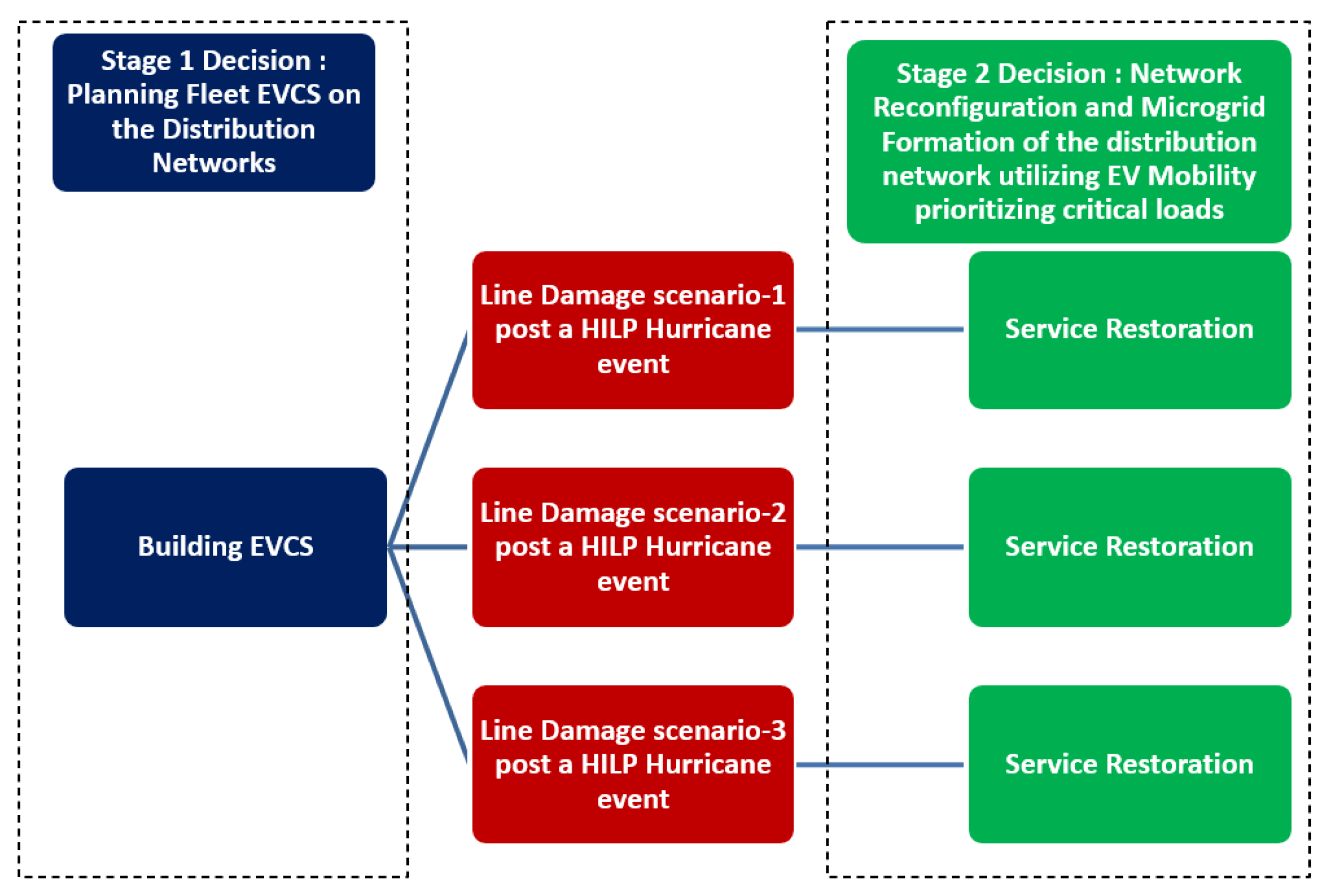
A two-stage stochastic optimization approach with a mixed-integer second-order cone programming (MISOCP) model is developed for the optimal siting of FEVCSs, considering EV mobility and the effects of extreme weather events. The first stage deals with the selection of the most favorable location for FEVCSs, whereas the second stage minimizes the weighted sum of the value of lost load (VOLL) under potential fault scenarios, integrating transportation network considerations into the grid restoration scheme.

3.

The study evaluates the influence of renewable-supported battery energy storage systems (BESSs) on the optimal placement of FEVCSs and demonstrates the potential of BESSs to improve the flexibility of the grid.

2. Problem Statement

The total storage capacity of a fleet of 20 medium- or heavy-duty EVs can reach 4 to 8 MWh. Since most trucks operate less than 5 h a day [2], such a fleet can dedicate some of its EVs to provide services to the grid to enhance the reliability and resilience of the power grid. HILP events, such as hurricanes, can lead to the failure of distribution network infrastructure, causing power outages in the network. Grid operators now have new options to resolve unplanned outages because of the proliferation of distributed resources on the grid. Utility services monitor significant weather events so that the maintenance teams can respond to potential faults in the distribution network; after a weather event has passed, several faults occur in a power distribution network. These faults can create multiple healthy and faulty sections in the network. A smart grid can use distributed energy resources (DERs) in the network to form microgrids and power the healthy sections of the network. EV fleet storage can be used to form and operate islanded networks, minimizing the effects of customer outages. Medium and heavy-duty EVs can opt to support the grid during HILP events. FEVCSs in strategic locations can enhance the resilience of the power distribution network. The time required by the vehicles to charge and move energy from one node to another should be considered. In this paper, the problem of strategically placing FEVCSs to enhance the resilience of the distribution network is modeled as a two-stage stochastic optimization model. Figure 1 presents the proposed two-stage stochastic optimization model.

A three-node transportation network and a 33-node distribution network for the second stage model is represented in Figure 2, which presents a scenario with faults on branches 7–8 and 26–27. The protection scheme on the distribution network is assumed to isolate faults using reclosers and circuit breakers. With the fault repairs in progress, the next step is to energize the maximum number of nodes. Microgrids can be established using DERs such as renewable generators, energy storage systems, and fleet vehicles. The mobility of fleet vehicles can be considered by using a transportation network. The fleet vehicles can act as BESSs or move energy from one microgrid to another during grid-service restoration via microgrid formation. In the scenario shown in Figure 2, three microgrids are used to power all the nodes of the distribution network. In the real world, there is some flexibility in the node that can be used to power an energy consumer. The problem addressed in this paper is to find the optimal location to connect FEVCS customers to the grid. Building FEVCSs at strategic locations can improve grid resilience while progressing toward the goal of reducing GHG emissions.

3. Mathematical Formulation

In this paper, a stochastic model is presented as a solution to a planning problem regarding the resilience of a distribution network. The first stage models the investment decision with options of hardening and the placement of FEVCS as methods to improve resilience. Line hardening involves the substitution of overhead lines and poles with underground cables, a modification aimed at mitigating the grid’s susceptibility to external disruptions and ensuring consistent and reliable power distribution. In the second stage, a joint grid restoration scheme with network reconfiguration and microgrid formation is modeled in the presence of DGs and fleet vehicles. Investing decisions in the first stage are based on the expected cost of load shedding, weighted by the probability distribution of line damage scenarios for the second stage.

3.1. First Stage: Distribution System Planning

The distribution planning model minimizes the investment cost required for the upgrade of the infrastructure as shown in (1). The options for investments to enhance the resilience provided are distribution line hardening of line l represented by $R_l$ and the installation of FEVCSs represented by $E_e$. In the third term, $N_H$ represents the number of HILP events in a year times the weighted sum based on the probability of the objective function of all fault scenarios in the second stage. Constraint (2) defines the budget limit in the investment of infrastructure. Constraint (3) indicates each EVCS can be assigned to only one bus.

$$\begin{array}{c}\hfill min\sum _l{C}_l^R\times R_l+\sum _e{C}_e^E\times E_e+N_H\times \sum _s{\pi }_s\times \rho \left(s\right)\end{array}$$

(1)

$$\begin{array}{c}\hfill \sum _l{C}_l^R\times R_l+\sum _e{C}_e^E\times E_e\le B\end{array}$$

(2)

$$\begin{array}{c}\hfill \sum _e{E}_e\le 1,\forall i\end{array}$$

(3)

3.2. Second Stage: Joint Restoration Scheme

In the event of a natural disaster that affects the grid, there may be line damages in the distribution network and also a failure in the supply from the transmission substation. Microgrids play a vital role in grid restoration during this crisis. The grid restoration scheme considered in the model uses a microgrid formation that incorporates available DGs and fleet vehicles. The objective function of the joint restoration scheme is to minimize the expected cost of load shedding, shown in (4).

$$\begin{array}{cc}\hfill \rho \left(s\right)=& min\sum _s\sum _t\sum _i(VoL{L}_i\times s_{i,t,s}^d)+\sum _s\sum _t\sum _j(l_{j,t,s}\times r_l)\hfill \end{array}$$

(4)

In the equation, $\rho \left(s\right)$ represents the objective function, which is a function of scenario s, and minimizes the sum of VOLL multiplied by the load shedding and $I^{2}r$ losses. $VoL{L}_i$ represents VOLL at node i, and $s_{i,t,s}^d$ represents the load shedding at node i in time t of scenario s. The constraints for the joint restoration scheme are network reconfiguration and microgrid formation, DG, time–space network (TSN), and fleet vehicle constraints.

3.2.1. Network Reconfiguration and Radiality Constraints

Network reconfiguration constraints define the switching action that segregates the nodes, ensuring the radiality of the microgrids. The binary variable $A_{i,m,s}$ will be one if the i-th node belongs to the microgrid $m\in S_M$ in the scenario $s\in S_S$. Here, $S_M$ represents the set of all microgrids and $S_S$ is the set of all scenarios considered in the second stage.

$$\begin{array}{c}\hfill A{r}_{i,s}=\sum _{m=1}^{S_M}{A}_{i,m,s}\le 1,\forall i,m,s\end{array}$$

(5)

The node i can be connected to microgrid m in scenario s if the m-th member of $S_{I_{DG}}$ is selected as the root bus.

$$\begin{array}{c}\hfill A_{i,m,s}\le A_{j,m,s},j\in S_{I_{DG}}\forall i,m,s\end{array}$$

(6)

The binary variable $O_{l,s}$ is set to zero if two nodes of a distribution line do not belong to the same microgrid. Meanwhile, $i^{\prime }$ represents the index for the terminal bus of line l. Equation (7) is linearized by applying linear methods to Equations (8)–(10). Equation (11) defines a binary variable $O_{l,s}$ that is 1 when the branch is active as part of any microgrid in scenario s.

$$\begin{array}{c}\hfill O_{l,s}\le A_{i,m,s}\times A_{i^{\prime },m,s},\forall i,i^{\prime },m,s\end{array}$$

(7)

$$\begin{array}{c}\hfill O_{l,m,s}\le \sum _i{A}_{i,m,s},i\in S_{IB},\forall l,m,s\end{array}$$

(8)

$$\begin{array}{c}\hfill O_{l,m,s}\le \sum _{i^{\prime }}{A}_{i^{\prime },m,s},i^{\prime }\in S_{TB},\forall l,m,s\end{array}$$

(9)

$$\begin{array}{cc}\hfill O_{l,m,s}\ge & \sum _i{A}_{i,m,s}+\sum _{i^{\prime }}{A}_{i^{\prime },m,s}-1,i\in S_{IB},i^{\prime }\in S_{TB}\forall l,m,s\hfill \end{array}$$

(10)

$$\begin{array}{c}\hfill O_{l,s}=\sum _{m\in S_M}{O}_{l,m,s},\forall l,s\end{array}$$

(11)

Constraints (12)–(14) represent the status of a line and a bus while considering damaged lines during a scenario using the binary variable $F_{l,s}$ and hardening in the first stage controlled by the binary variable $R_l$. Equation (12) controls the effect of hardening on line damage. Equations (13) and (14) ensure that the health status of the line and bus generated during the line damage scenario is applied to the model.

$$\begin{array}{c}\hfill O_{l,s}\le 1-(1-F_{l,s})\times (1-R_l),\forall l,s\end{array}$$

(12)

$$\begin{array}{c}\hfill O_{l,m,s}\le L{H}_{l,s},\forall l,m,s\end{array}$$

(13)

$$\begin{array}{c}\hfill A_{i,m,s}\le B{H}_{i,s},\forall i,m,s\end{array}$$

(14)

The radiality of each distribution network is ensured by utilizing a necessary and sufficient condition from [18]. The necessary condition requires the number of buses minus the number of branches to be equal to one, which is ensured using Constraints (15)–(17). The sufficient condition is to ensure connectivity of each microgrid, which is included in the model employing Constraints (18)–(21). The binary variable ${\xi }_{m,s}$ is one if microgrid m is selected. Meanwhile, ${\beta }_{i,i^{\prime },l,m,s}$ represents the fictional flow on line l with nodes $i\&i^{\prime }$. Finally, ${\beta }_{i^{\prime },m,s}^{\left(2\right)}$ represents the fictional supply of master DG m.

$$\begin{array}{c}\hfill \sum _i{A}_{i,m,s}\le M\times {\xi }_{m,s},\forall l,s\end{array}$$

(15)

$$\begin{array}{c}\hfill {\xi }_{m,s}\le M\times \sum _i{A}_{i,m,s},\forall l,s\end{array}$$

(16)

$$\begin{array}{c}\hfill \sum _l{O}_{l,m,s}=\sum _i{A}_{i,m,s}-{\xi }_{m,s},\forall l,s\end{array}$$

(17)

$$\begin{array}{cc}\hfill \sum _{i\in S_{TB}}& \sum _l{\beta }_{i,i^{\prime },l,m,s}^{\left(1\right)}-\sum _{i\in S_{IB}}\sum _l{\beta }_{i,i^{\prime },l,m,s}^{\left(1\right)}=A_{i^{\prime },m,s},i^{\prime }\ne S_{I_{DG}}\forall m,s\hfill \end{array}$$

(18)

$$\begin{array}{cc}\hfill \sum _{i\in S_{TB}}& \sum _l{\beta }_{i,i^{\prime },l,m,s}^{\left(1\right)}-\sum _{i\in S_{IB}}\sum _l{\beta }_{i,i^{\prime },l,m,s}^{\left(1\right)}=-{\beta }_{i^{\prime },m,s}^{\left(2\right)},i^{\prime }=S_{I_{DG}}\forall m,s\hfill \end{array}$$

(19)

$$-O_{l,m,s}\times M\le {\beta }_{i,i^{\prime },l,m,s}^{\left(1\right)}\le O_{l,m,s}\times M, i\in S_{TB},i^{\prime }\in S_{IB}\forall l,m,s$$

(20)

$$A_{i^{\prime },m,s}\le {\beta }_{i^{\prime },m,s}^{\left(2\right)}\le M\times A_{i^{\prime },m,s},i^{\prime }\in S_{I_{DG}}\forall m,s$$

(21)

3.2.2. DG Constraints

DGs are used via microgrids as the primary source of energy during restoration to reduce the load shedding. Equations (22)–(24) model the DG’s active, reactive, and apparent power limits.

$$\begin{array}{c}\hfill 0\le P_{g,t}^{DG}\le P_g^{DG,max}\end{array}$$

(22)

$$\begin{array}{c}\hfill -Q_g^{DG,max}\le Q_{g,t}^{DG}\le Q_g^{DG,max}\end{array}$$

(23)

$$\begin{array}{c}\hfill ∥P_{g,t}^{DG}{Q}_{g,t}^{DG}∥\le S_g^{DG,max}\end{array}$$

(24)

3.2.3. Time–Space Network Constraints

The TSN model is used to represent the movement of fleet vehicles along the grid during a disaster [10]. The binary variable $G_{f,e{e}^{\prime },t}$ is one if the vehicle f is on an arc from FEVCS e to $e^{\prime }$ during time t. Constraint (25) models undergo movement during a period of time. Equation (26) models the relationship between the state of a vehicle and the progression of time. Equation (27) defines the initial position of the vehicles.

$$\begin{array}{c}\hfill G_{f,e{e}^{\prime },t}=1,\forall f\in S_F,t\in T\end{array}$$

(25)

$$\begin{array}{cc}\hfill \sum _{(m,e^{\prime })\in K_m^{-}}{G}_{f,e{e}^{\prime },t}& =\sum _{(m,e^{\prime })\in K_m^{+}}{G}_{f,e{e}^{\prime },t+1},\forall f\in S_F,e\in S_{EVCS}\cup S_V,t\in T\hfill \end{array}$$

(26)

$$\begin{array}{c}\hfill \sum _{(m,e^{\prime })\in K_m^{+}}{G}_{f,e{e}^{\prime },1}=G_{f,e}^0,\forall f\in S_F,e\in S_{EVCS}\cup S_V\end{array}$$

(27)

3.2.4. Operational Constraints of Fleet Vehicles

If $E_e$ is a binary variable which represents the choice to build an FEVCS at the candidate location node e, then ${\gamma }_{e,s}$ is the binary variable that represents an active node during microgrid formation with an FEVCS installed at node e. Equation (28) is linearized using (29)–(31).

$$\begin{array}{c}\hfill {\gamma }_{e,s}=A{r}_{e,s}\times E_{e,s},\forall e,s\end{array}$$

(28)

$$\begin{array}{c}\hfill {\gamma }_{e,s}\le A{r}_{e,s},\forall e,s\end{array}$$

(29)

$$\begin{array}{c}\hfill {\gamma }_{e,s}\le E_{e,s},\forall e,s\end{array}$$

(30)

$$\begin{array}{c}\hfill {\gamma }_{e,s}\ge E_{e,s}+A_{e,s}-1,\forall e,s\end{array}$$

(31)

Similarly, ${\alpha }_{f,e,t,s}$ connects the active EVCS node to the fleet vehicle’s movement along the grid. The variable $G_{f,ee,t,s}$ represents the active arc $ee$ of the fleet vehicle f at a time t in the scenario, where s means that the vehicle is connected to a node e of the TSN. Constraint (32) is linearized using (33)–(35).

$$\begin{array}{c}\hfill {\alpha }_{f,e,t,s}={\gamma }_{e,s}\times G_{f,ee,t,s},\forall f,s\end{array}$$

(32)

$$\begin{array}{c}\hfill {\alpha }_{f,e,t,s}\le {\gamma }_{e,s},\forall f,s\end{array}$$

(33)

$$\begin{array}{c}\hfill {\alpha }_{f,e,t,s}\le G_{f,ee,t,s},\forall f,s\end{array}$$

(34)

$$\begin{array}{c}\hfill {\alpha }_{f,e,t,s}\ge G_{f,ee,t,s}+{\gamma }_{e,s}-1,\forall f,s\end{array}$$

(35)

The charging and discharging of fleet vehicles are represented by Constraints (36)–(47). Constraints (36) and (37) restrict the charging and discharging of fleet vehicles to happen only at an active node with FEVCS when the vehicle is on the arc $e-e$. Constraints (38)–(40) control the charging or discharging of vehicles over a period of time. Constraint (41) defines a single variable that represents the power transfer of the fleet vehicle. Constraint (42) represents the apparent power limit of the fleet vehicles.

$$\begin{array}{c}\hfill 0\le P_{f,e,t,s}^{FV,ch}\le {\alpha }_{f,e,i,s}\times P_e^{EVCS,max},\forall f,t,s\end{array}$$

(36)

$$\begin{array}{c}\hfill 0\le P_{f,e,t,s}^{FV,dch}\le {\alpha }_{f,e,i,s}\times P_e^{EVCS,max},\forall f,t,s\end{array}$$

(37)

$$\begin{array}{c}\hfill 0\le P_{f,e,t,s}^{FV,ch}\le Y_{f,t,s}^{ch}\times P_e^{EVCS,max},\forall f,t,s\end{array}$$

(38)

$$\begin{array}{c}\hfill 0\le P_{f,e,t,s}^{FV,dch}\le Y_{f,t,s}^{dch}\times P_e^{EVCS,max},\forall f,t,s\end{array}$$

(39)

$$\begin{array}{c}\hfill Y_{f,t,s}^{dch}+Y_{f,t,s}^{ch}\le {\alpha }_{f,e,i,s},\forall f,t,s\end{array}$$

(40)

$$\begin{array}{c}\hfill P_{f,e,t,s}^{FV}=\frac{P_{f,e,t,s}^{FV,dch}}{{\eta }^{dch}}-{\eta }^{dch}{P}_{f,e,t,s}^{FV,ch},\forall f,t,s\end{array}$$

(41)

$$\begin{array}{c}\hfill ∥P_{f,e,t,s}^{FV}{Q}_{f,e,t,s}^{FV,dch}∥\le {\alpha }_{f,e,i,s}\times S_f^{EVCS,max}\end{array}$$

(42)

The constraints related to the state of charge (SOC) of the fleet vehicles are modeled in (43)–(47). Constraint (43) defines the relationship of the initial SOC of the EV with a SOC of the second hour, which is activated by ${\alpha }_{f,e,t,s}$. Constraint (44) defines the relationship of the SOC of the EV when t is not equal to one. The relationship between the SOC of the EV when the EV is not connected to an FEVCS is shown in (45) and (46). The upper and lower limit of the SOC of the EV is defined in Constraint (47).

$$\begin{array}{cc}\hfill -M& (1-{\alpha }_{f,e,t,s})\le SO{C}_{Initial}^{FV}-SO{C}_{f,t,s}^{FV}-P_{f,e,t+1,s}^{FV}\le M(1-{\alpha }_{f,e,t,s}),\forall f,t=1,s\hfill \end{array}$$

(43)

$$\begin{array}{cc}\hfill -M& (1-{\alpha }_{f,e,t,s})\le SO{C}_{f,t-1,s}^{FV}-SO{C}_{f,t,s}^{FV}-P_{f,e,t+1,s}^{FV}\le M(1-{\alpha }_{f,e,t,s}),\forall f,t\ne 1,s\hfill \end{array}$$

(44)

$$\begin{array}{cc}\hfill -M& \sum _e{\alpha }_{f,e,t,s}\le SO{C}_{Initial}^{FV}-SO{C}_{f,t,s}^{FV}-P_{f,e,t+1,s}^{FV}\le M\sum _e{\alpha }_{f,e,t,s},\forall f,t=1,s\hfill \end{array}$$

(45)

$$\begin{array}{cc}\hfill -M& \sum _e{\alpha }_{f,e,t,s}\le SO{C}_{f,t-1,s}^{FV}-SO{C}_{f,t,s}^{FV}-\times P_{f,e,t+1,s}^{FV}\le M\sum _e{\alpha }_{f,e,t,s},\forall f,t\ne 1,s\hfill \end{array}$$

(46)

$$\begin{array}{c}\hfill SO{C}_f^{min}\le SO{C}_{f,t+1,s}\le SO{C}_f^{max},\forall f,t,s\end{array}$$

(47)

3.2.5. Power Flow Constraints

The nodal active power balance is modeled using Constraint (48) [18]. Since $p_{f,e,t,s}^{FV}$ in (48) is the product of $P_{f,e,t,s}^{FV}$ and ${\alpha }_{f,e,t,s}$, Constraints (49)–(51) are used to linearize the equation. Constraints (52) and (53) define the decision variables for switchable loads. Constraint (54) defines a decision variable to represent load shedding at each node in each scenario.

$$\begin{array}{cc}\hfill & \sum _{i\in N1\left(j\right)}(p_{ij,t}-l_{ij,t}{r}_{ij})-\sum _{k\in N2\left(j\right)}{p}_{jk,t}+\sum _{m\in S_M}\left[\sum _{g\in S_G}{P}_{g,t}^{DG}+\sum _{f\in S_{FV}}{p}_{f,e,t,s}^{FV}-p_{j,t}^d\right]=0\hfill \end{array}$$

(48)

$$\begin{array}{c}\hfill p_{f,e,t,s}^{FV}\le P_e^{EVCS,max},\forall f,t,s\end{array}$$

(49)

$$\begin{array}{c}\hfill p_{f,e,t,s}^{FV}\le P_{f,e,t,s}^{FV},\forall f,t,s\end{array}$$

(50)

$$\begin{array}{c}\hfill p_{f,e,t,s}^{FV}\ge P_{f,e,t,s}^{FV}-P_e^{EVCS,max},\forall f,t,s\end{array}$$

(51)

$$\begin{array}{c}\hfill p_{j,t}^d=A{r}_{j,s}\times D_{j,t}^P,\forall j,t,s\end{array}$$

(52)

$$\begin{array}{c}\hfill q_{j,t}^d=A{r}_{j,s}\times D_{j,t}^Q,\forall j,t,s\end{array}$$

(53)

$$\begin{array}{c}\hfill s_{j,t}^d=D_{j,t}^P-p_{j,t}^d,\forall j,t,s\end{array}$$

(54)

Similarly, the nodal reactive power balance is modeled using Constraint (55), which is linearized by (56)–(58).

$$\begin{array}{cc}\hfill & \sum _{i\in N1\left(j\right)}(q_{ij,t}-l_{ij,t}{x}_{ij})-\sum _{k\in N2\left(j\right)}{q}_{jk,t}+\sum _{m\in S_M}\left[\sum _{g\in S_G}{Q}_{g,t}^{DG}+\sum _{f\in S_{FV}}{q}_{f,e,t,s}^{FV}-q_{j,t}^d\right]=0\hfill \end{array}$$

(55)

$$\begin{array}{c}\hfill q_{f,e,t,s}^{FV}\le Q_e^{EVCS,max},\forall f,t,s\end{array}$$

(56)

$$\begin{array}{c}\hfill q_{f,e,t,s}^{FV}\le Q_{f,e,t,s}^{FV,dch},\forall f,t,s\end{array}$$

(57)

$$\begin{array}{c}\hfill q_{f,e,t,s}^{FV}\ge Q_{f,e,t,s}^{FV,dch}-Q_e^{EVCS,max},\forall f,t,s\end{array}$$

(58)

The upper and lower limits for nodal voltages of active nodes are modeled using (59). The voltages of the master DGs are set using Constraint (60). The nodal voltage drop constraints bound via the Big-M method are modeled using (61). The relation between power flow, current, and voltage is defined using (62). Constraint (63) is used to model the limits of branch current flow in the distribution network. Constraints (64) and (65) model the active and reactive power flow through the closed branches of the distribution network.

$$\begin{array}{c}\hfill A_{i,m,s}\times {\left(V_{(i,min)}\right)}^2\le u_{i,t}\le A_{i,m,s}\times {\left(V_{(i,max)}\right)}^2,\forall i,t,s\end{array}$$

(59)

$$\begin{array}{c}\hfill u_{i,t}=A_{i,m,s}\times {\left(V_m^{DG,set}\right)}^2,\forall i\in S_{I_{DG}},\forall i,t,s\end{array}$$

(60)

$$\begin{gathered} \begin{array}{cc}\hfill -M& \times (1-O_{l,s})\le u_{i,t,s}-u_{j,t,s}-2(r_{ij}{p}_{ij,t}+x_{ij}{q}_{ij,t})+({\left(r_{ij}\right)}^2+{\left(x_{ij}\right)}^2)l_{ij,t}\le \hfill \end{array} \\ \begin{array}{c}\hfill M\times (1-O_{l,s}),\forall l,t,s\end{array} \end{gathered}$$

(61)

$$\begin{array}{c}\hfill ∥2p_{ij,t}2q_{ij,t}(l_{ij,t}-u_{i,t})∥\le (l_{ij,t}+u_{i,t})\end{array}$$

(62)

$$\begin{array}{c}\hfill 0\le l_{l,t,s}\le O_{l,s}\times {\left(I^{Max}\right)}^2,\forall l,t,s\end{array}$$

(63)

$$\begin{array}{c}\hfill -O_{l,s}\times \left(p_{ij}^{Max}\right)\le p_{ij,t,s}\le O_{l,s}\times \left(p_{ij}^{Max}\right),\forall i,t,s\end{array}$$

(64)

$$\begin{array}{c}\hfill -O_{l,s}\times \left(q_{ij}^{Max}\right)\le q_{ij,t,s}\le O_{l,s}\times \left(q_{ij}^{Max}\right),\forall i,t,s\end{array}$$

(65)

The model of BESS used in [19] was used to represent the behavior of BESS during grid service restoration.

Objective function (1) constrained by (2) and (3) forms the stage 1 model of the two-stage stochastic model. Stochastic objective function (4) constrained by (5)–(65) forms the MISOCP stage 2 of the two-stage stochastic problem. Combined objective functions of both the above-mentioned stages constrained by their respective constraints form the two-stage stochastic optimization approach with a MISOCP model. In a two-stage stochastic model, the first stage makes decisions before the realization of uncertainty, creating a framework for optimal decision making, while the second stage adapts these decisions post-realization, ensuring a robust and flexible response to various possible scenarios.

3.3. Scenario Generation and Reduction

Figure 1 shows that the distribution network’s line damage scenarios post-HILP event links the first stage to the second stage of the model. Since hurricanes are addressed in the problem, the wind speed data from Atlantic Oceanographic and Meteorological Laboratory’s hurricane database [20] was fed into a custom PDF sampler and reconstructor by Pantelis Sopasakis [21]. This custom PDF reconstructor was used to generate wind speeds that create hurricane wind speeds. Fragility functions from [15] were employed to generate 100 line damage scenarios. The program scenred [22] was used to reduce the 100 scenarios to three scenarios.

4. Numerical Results

4.1. Feeder and Case Description

The model was tested on a modified IEEE-33 node distribution network and a four-node transportation network, as shown in Figure 3. The feeder has residential loads connected to nodes 1–22, commercial loads from nodes 22 to 33, and a hospital at node 30. Figure 4 shows the load profiles used for the different load types. The loads and VOLL for all the nodes in the case are shown in Figure 5. The 33-node network is divided into four zones, shown as Z1, Z2, Z3, and Z4 in Figure 3. The distributed generation available in the network includes three solar farms across nodes 18, 22, and 25, and a conventional gas generator of 1 MW at node 33. A candidate node from each zone was selected as a potential FEVCS location. The selected candidate nodes for FEVCS are presented as nodes connected by a road network in the figure. Nodes 18, 22, 25, and 33 were selected as the search window for the optimal location of the FEVCS. It is assumed that the fault is active for 8 h, and during a fault, the upstream substation does not provide power to the network. Furthermore, it is assumed that the FEVCS has more than three charging ports available for the support of grid restoration. Only three representative EVs—several fleets of EVs with the same routing behavior—are considered in all cases to incorporate the variation in usable EV storage with a minimal computational load. Moreover, the size of the chargers can be varied to incorporate the increase or decrease in usable EV storage; the considered FEVCS is made up of 125 kW capacity chargers, vehicles are considered to have usable storage of 300 kWh each, and six fleet vehicles are considered available for grid restoration. To reduce the computational load, two fleet vehicles are assumed to follow the same behavior; therefore, the representative EV considered for the base cases has a storage of 600 kWh and a charger rating of 250 kW. Cases 0, 1, and 2 are cases with zero, one, and two FEVCSs on the distribution network, respectively. The aforementioned cases do not have any BESS in the network. Cases 3, 4, and 5 are cases with zero, one, and two FEVCSs with solar farms supported by BESS. The probabilities of the line damage scenarios after scenario reduction are 0.277, 0.388, and 0.333 respectively. The results of scenario 2 of the second stage are presented as it is the most probable scenario and will have the most influence, while the first stage model decides the location of the FEVCS. The rest of the scenarios do not have faults that interrupt the power flow to cause any load loss. In the analysis below, the SOC has been mentioned in terms of stored energy in kWh.

4.2. Simulation Results and Analysis

The results of the distribution system planning model presented in Section 3.1 are based on the stochastic objective function of all three scenarios of the joint restoration scheme presented in Section 3.2. As the scenario with the highest probability, scenario 2 is used to present the results and analysis of the second stage of the model. The faults in scenario 2 are on branches 16–17, 17–18, 21–22, 6–26, 9–15, and 22–12. The model’s response to these faults for Case 0 is shown in Figure 6. Acting as the grid forming generator, the gas turbine generator GT4 forms microgrid MG4 energizing the loads on nodes 18 and 26–33. While GT4 acts as the master generator in MG4, the PV generator PV1 acts as a slave generator providing active power when available and reactive power support to improve the voltage of the system.

4.2.1. Case 1: Optimal Location of the FEVCS

The optimal location of the first FEVCS for the presented network is node 25. As shown in Figure 7, nodes 18 and 25–33 are active during the fault. As there are no other EVCSs in this case, node 25 was selected because the FEVCS can act as energy storage to power node 25, which was added to the active grid because the VOLL of the nodes in zones Z3 and Z4 is higher. Figure 8 shows the generation, load, and vehicle-to-grid during the fault. The SOC of the fleet vehicles and the power of vehicle-to-grid is shown in Figure 9. In Section 4.2.2, the model solves the problem of the second-best location for the FEVCS of the network in the presence of an FEVCS at node 25.

4.2.2. Case 2: Second-Best Location for FEVCS

The second-best location of the FEVCS is estimated to be at node 22. In Case 2, FEVCSs at nodes 22 and 25 act as energy storage for the grid; compared with Case 1, one more node is active in the network, reducing the VOLL of Case 1. The mobility of the fleet vehicles is presented in

Table 2. Mobility of fleet vehicles in the transportation network in Case 2.

	Time
	15:00	16:00	17:00	18:00	19:00	20:00	21:00
EV#1	2-3	3-2	2-3	3-3	3-3	3-3	3-3
EV#2	1-1	1-2	2-2	2-2	2-3	3-3	3-3
EV#3	4-3	3-3	3-3	3-2	2-2	2-2	2-2

. As shown in the Figure 10, two master DGs form microgrids MG2 and MG3 to energize the active grid sections. While the generators PV2 and PV3 act as master DGs, GT4 follows the generator PV3. Moreover, both FEVCSs support the mircogrids in moving energy from an energy surplus microgrid to an energy deficient microgrid. The fleet vehicle EV-1 is not used for restoration during 14:00–16:00 h; instead, the vehicle is located at node 3 of the transportation network, which overlaps with the distribution network at node 25. From Figure 11, EV-1 is used from 18:00 to 21:00 h, during which the storage of EV-1 reduces to the minimum value. Mobility is used by the model for vehicles EV-2 and EV-3. The demand to upkeep microgrid 3, controlled by the DG at node 25, is higher than the demand for microgrid 2, controlled by node 22. Therefore, the model uses EV-3 at node 25 for 16:00 to 17:00 h and then sends EV-3 to node 22 because the available storage cannot provide sufficient energy to node 25. Then EV-2, which has higher storage, is used to energize node 25 to provide sufficient energy to manage the supply–demand balance of the presented configurations.

4.2.3. Effects of BESS on the FEVCS Location

A BESS of 1 MW capacity and 2.5 MWh storage was added to all solar farms in Cases 0, 1, and 2 to obtain Cases 3, 4, and 5. The network configuration of the restored grid is presented in Figure 12. The active nodes in the restored distribution network have increased from Case 2. In Case 4, the model solved the optimal location of the FEVCS in the presence of renewables backed by the BESS. The optimal location of the FEVCS is node 25 in the distribution network.

Figure 13 shows that, when compared to Case 3, Case 4 adds node 24 and sheds node 26. Node 24 has a higher VOLL compared to node 26 because of the commercial load capacity on node 26. Compared with Case 2, EV-1 and EV-2 charge when there is surplus energy during some hours to support the grid during other hours. As shown in Figure 14, EV-1 discharges during 17:00 h, charges during 18:00 h, and discharges during 19:00–21:00 h. Adding a BESS for the solar farm at node 25 has provided the network with this flexibility compared with Case 2.

The model solved the problem in Case 5 for the best two locations for the FEVCS on the presented network in the presence of renewables backed by BESS, with a MIPGap of 0.13%. The best two locations for the FEVCSs are node 25 and node 22. In comparison to Case 4, Case 5 powers a lower number of nodes because the model prioritizes loads with higher VOLL. Both microgrids have one FEVCS each. The configuration after service restoration of the distribution network in Case 5 is shown in Figure 15.

Table 3. Mobility and SOC of fleet vehicles in the transportation network in Case 5.

	Time
	15:00	16:00	17:00	18:00	19:00	20:00	21:00
EV#1	1-4	4-3	3-3	3-3	3-2	2-2	2-2
EV1_SOC (kWh)	600.0	600.0	350.0	100.0	100.0	81.8	56.3
EV#2	2-3	3-3	3-2	2-2	2-3	3-3	3-3
EV2_SOC (kWh)	600.0	350.0	350.0	555.8	555.8	305.8	55.8
EV#3	2-2	2-2	2-3	3-3	3-3	3-3	3-4
EV3_SOC (kWh)	513.3	600.0	600.0	427.6	216.8	50.0	50.0

shows the mobility and variation in the SOC of the EVs. EV-1 is called to node 3 at 16:00 h. At 17:00 h, EV-1 is in the arc 3-3 of the TSN, indicating that EV-1 is connected to node 3 of the transportation network, which is node 25 of the power distribution network. EV-1 discharges at 17:00 and 18:00 h, supporting microgrid 3. At 19:00 h, EV-1 is called to node 2 to support microgrid 2 during 20:00–21:00 h. EV-2 is called to node 25 at 15:00 h, discharges at node 25 to support microgrid 3, and is called to node 22 to charge from microgrid 2 at 18:00 h. EV-2 goes back to node 25 during 19:00 h and supports microgrid 3 in 20:00 and 21:00 h. EV-2 transports energy from microgrid 2 to microgrid 3 to power more critical loads on microgrid 2. Similarly, EV-3 is called to node 22 at 14:00 h. EV-3 supports microgrid 2 during 15:00 h, recharges during 16:00 h, and supports microgrid 3 during 18:00–20:00 h. Figure 16 shows the variation in the objective function for all cases. Adding a BESS to the mix has increased the effects of the FEVCS in improving the objective function.

4.3. MISOCP Relaxation Gap and Simulation Setup

The accuracy of MISOCP relaxation was tested to compare the power flow obtained from conic relaxation with the original nonconvex model by evaluating the relaxation error defined as

$$Gap=ma{x}_{\forall (i,j)}\left|p_{ij}^2+q_{ij}^2-\left(l_{ij}{u}_i\right)\right|$$

(66)

The SOC gap for the case is the order of ${10}^{-9}$ MW. Simulations were carried out on an Apple Macbook with 32 GB RAM and an Apple M2 Pro CPU with 12 cores. The problem was modeled using MathWorks’ MATLAB with YALMIP and Gurobi addons. The MIPGap and the solution time of all simulated cases are shown in

Table 4. MIPGap (%) and solution time.

Case	MIP GAP	Solution Time (hours)
0	0	0.004
1	0	0.261
2	0.001	17.534
3	0	0.597
4	0.078	55.437
5	0.13	70.579

. In the context of the presented results, “MIPGap” is a parameter set to define the tolerance level for the difference between the lower and upper objective bounds, allowing the algorithm to terminate once this relative gap is attained, thereby ensuring that the obtained solution is close to optimality within this threshold.

5. Conclusions and Future Works

The present study provides a comprehensive assessment of a two-stage stochastic model for optimizing the location of the FEVCS within a distribution network. This innovative approach aims to improve network resilience and reliability, particularly during operational faults or disaster management scenarios. The model was thoroughly tested on a modified IEEE-33 node distribution network and a four-node transportation network, which included various types of loads and DGs.

The optimal location of the FEVCS, as identified by the model, was at node 25. This node was selected because of its potential to act as energy storage for powering the node and its influence on zones Z3 and Z4 with higher VOLL. Furthermore, the second-best location was determined to be node 22, which added an active node to the network and reduced VOLL compared with the first case. This scenario also showed a strategic use of the mobility and storage capabilities of the fleet vehicles, providing an energy supply–demand balance.

In addition, renewable generators supported by a BESS were also considered. The model demonstrated an increased number of active nodes in the restored distribution network, with the optimal FEVCS location remaining at node 25. The presence of the BESS allowed for greater flexibility in the network, allowing the vehicles to charge during periods of surplus energy and support the grid during other hours. When two FEVCSs were present alongside BESS-backed renewables, the model prioritized loads with higher VOLL, resulting in powering a fewer number of nodes, but catering to more critical loads.

The proposed stochastic model presents a potential path for strategic planning and optimization of the FEVCS in a distribution network, enhancing the resilience and reliability of the network. The results highlight the valuable role of an FEVCS, particularly when combined with a BESS, in responding to network faults and managing supply–demand balances. Future work further explores other factors that influence the model and test the model on larger or more complex network configurations and to use a stochastic distribution control approach to assess the robustness of the optimization by controlling the probability density function (PDF) shape of the concerned objective functions. In this context, the narrower and sharper PDF of the optimized objective functions would indicate the strong robustness of the optimization.

References

1. U.S. Environmental Protection Agency. Fast Facts on Transportation Greenhouse Gas Emissions. Available online: https://www.epa.gov/greenvehicles/fast-facts-transportation-greenhouse-gas-emissions (accessed on 5 June 2023).
2. National Renewable Energy Laboratory. Fleet DNA Project Data Summary Report. Available online: https://www.nrel.gov/transportation/assets/pdfs/fleet_dna_delivery_trucks_report.pdf (accessed on 16 January 2023).
3. Atlas Public Policy. U.S. Medium- and Heavy-Duty Truck Electrification Infrastructure Assessment. Available online: https://atlaspolicy.com/u-s-medium-and-heavy-duty-truck-electrification-infrastructure-assessment/ (accessed on 16 January 2023).
4. Chargepoint. Electric Vehicle (EV) Charging Incentives. Available online: https://www.chargepoint.com/incentives/commercial?type=13&state=45 (accessed on 16 January 2023).
5. Panteli, M.; Trakas, D.N.; Mancarella, P.; Hatziargyriou, N.D. Power systems resilience assessment: Hardening and smart operational enhancement strategies. Proc. IEEE 2017, 105, 1202–1213. [Google Scholar] [CrossRef]
6. Hussain, A.; Musilek, P. Resilience Enhancement Strategies For and Through Electric Vehicles. Sustain. Cities Soc. 2022, 80, 103788. [Google Scholar] [CrossRef]
7. Brown, M.A.; Soni, A. Expert perceptions of enhancing grid resilience with electric vehicles in the United States. Energy Res. Soc. Sci. 2019, 57, 101241. [Google Scholar] [CrossRef]
8. Ahmadi, S.E.; Marzband, M.; Ikpehai, A.; Abusorrah, A. Optimal stochastic scheduling of plug-in electric vehicles as mobile energy storage systems for resilience enhancement of multi-agent multi-energy networked microgrids. J. Energy Storage 2022, 55, 105566. [Google Scholar] [CrossRef]
9. Yao, F.; Wang, J.; Wen, F.; Zhao, J.; Zhao, X.; Liu, W. Resilience Enhancement for a Power System with Electric Vehicles under Extreme Weather Conditions. In Proceedings of the 2019 IEEE Innovative Smart Grid Technologies-Asia (ISGT Asia), Chengdu, China, 21–24 May 2019; pp. 3674–3679. [Google Scholar]
10. Yao, S.; Wang, P.; Zhao, T. Transportable energy storage for more resilient distribution systems with multiple microgrids. IEEE Trans. Smart Grid 2018, 10, 3331–3341. [Google Scholar] [CrossRef]
11. Erenoğlu, A.K.; Sancar, S.; Terzi, İ.S.; Erdinç, O.; Shafie-khah, M.; Catalão, J.P. Resiliency-Driven Multi-Step Critical Load Restoration Strategy Integrating On-Call Electric Vehicle Fleet Management Services. IEEE Trans. Smart Grid 2022, 13, 3118–3132. [Google Scholar] [CrossRef]
12. Ma, S.; Chen, B.; Wang, Z. Resilience enhancement strategy for distribution systems under extreme weather events. IEEE Trans. Smart Grid 2016, 9, 1442–1451. [Google Scholar] [CrossRef]
13. Nazemi, M.; Moeini-Aghtaie, M.; Fotuhi-Firuzabad, M.; Dehghanian, P. Energy storage planning for enhanced resilience of power distribution networks against earthquakes. IEEE Trans. Sustain. Energy 2019, 11, 795–806. [Google Scholar] [CrossRef]
14. Dehghani, N.L.; Jeddi, A.B.; Shafieezadeh, A. Intelligent hurricane resilience enhancement of power distribution systems via deep reinforcement learning. Appl. Energy 2021, 285, 116355. [Google Scholar] [CrossRef]
15. Ghasemi, M.; Kazemi, A.; Gilani, M.A.; Shafie-Khah, M. A stochastic planning model for improving resilience of distribution system considering master-slave distributed generators and network reconfiguration. IEEE Access 2021, 9, 78859–78872. [Google Scholar] [CrossRef]
16. Faramarzi, D.; Rastegar, H.; Riahy, G.; Doagou-Mojarrad, H. A three-stage hybrid stochastic/IGDT framework for resilience-oriented distribution network planning. Int. J. Electr. Power Energy Syst. 2023, 146, 108738. [Google Scholar] [CrossRef]
17. Poudyal, A.; Poudel, S.; Dubey, A. Risk-based active distribution system planning for resilience against extreme weather events. IEEE Trans. Sustain. Energy 2022, 14, 1178–1192. [Google Scholar] [CrossRef]
18. Ding, T.; Lin, Y.; Bie, Z.; Chen, C. A resilient microgrid formation strategy for load restoration considering master-slave distributed generators and topology reconfiguration. Appl. Energy 2017, 199, 205–216. [Google Scholar] [CrossRef]
19. Ravi, A.; Bai, L.; Cecchi, V.; Ding, F. Stochastic Strategic Participation of Active Distribution Networks with High-Penetration DERs in Wholesale Electricity Markets. IEEE Trans. Smart Grid 2023, 14, 1515–1527. [Google Scholar] [CrossRef]
20. NOAA’s Atlantic Oceanographic & Meteorological Laboratory. Hurricane Database. Available online: https://www.aoml.noaa.gov/hrd/hurdat/hurdat2.html (accessed on 16 July 2021).
21. Sopasakis, P. PDFsampler. 2023. Available online: https://www.mathworks.com/matlabcentral/fileexchange/41689-pdfsampler (accessed on 20 January 2023).
22. Scenred. 2023. Available online: https://github.com/supsi-dacd-isaac/scenred (accessed on 20 January 2023).
Figure 1. Two-stage stochastic optimization model.
Applsci 13 12181 g001
Figure 2. Service restoration using DERs.
Applsci 13 12181 g002
Figure 3. Four-node transportation and IEEE-33 distribution network of the test case.
Applsci 13 12181 g003
Figure 4. Load profiles for different load types.
Applsci 13 12181 g004
Figure 5. Load and VOLL for different nodes.
Applsci 13 12181 g005
Figure 6. Grid service restoration by microgrid formation for fault in Scenario 2, Case 0.
Applsci 13 12181 g006
Figure 7. Grid service restoration by microgrid formation for fault in Scenario 2, Case 1.
Applsci 13 12181 g007
Figure 8. Generation load balance in microgrid 3 with optimal EVCS in Case 1.
Applsci 13 12181 g008
Figure 9. Variation in SOC and charging power of fleet EVs in Case 1.
Applsci 13 12181 g009
Figure 10. Grid service restoration by microgrid formation for fault in Scenario 2, Case 2.
Applsci 13 12181 g010
Figure 11. Variation in SOC and charging power of fleet EVs in Case 2.
Applsci 13 12181 g011
Figure 12. Grid service restoration in fault for Scenario 2, Case 3.
Applsci 13 12181 g012
Figure 13. Grid service restoration in fault for Scenario 2, Case 4.
Applsci 13 12181 g013
Figure 14. Variation in SOC and charging power of fleet EVs in Case 4.
Applsci 13 12181 g014
Figure 15. Grid service restoration in fault for Scenario 2, Case 5.
Applsci 13 12181 g015
Figure 16. Objective function of Cases 0–5.
Applsci 13 12181 g016