1. Introduction
Autonomous driving is a future-oriented technology with broad markets and development prospects. With the development of artificial intelligence and automation, in the automotive field, active safety systems in vehicles make transportation more efficient and safe [
1]. Nowadays, more and more vehicles are equipped with Advance Driver-Assistance Systems (ADASs). And among the subtasks of ADASs, drivable area segmentation is one of the important issues in all situations. The goal of drivable road segmentation is to sense the surrounding environment, keeping vehicles within safe road boundaries and preventing potential accidents, such as collisions with pedestrians or other vehicles in the driver’s blind spot [
2]. Therefore, it is fundamental to perceive complex scenarios and discern the drivable areas while driving.
In the past, most studies focused on the inaccurate road segmentation caused by the obstruction of other pedestrians or vehicles, or camera imaging distortion due to underexposure or halo effects. In the beginning, traditional image processing methods including edge-based, texture-classification-based, illuminant-invariance-based, and geometric-vanish-point-based methods were proposed [
3]. In the subsequent years, machine learning classifiers were applied to the field of drivable area segmentation, such as the SVM method [
4]. However, both image processing and machine learning methods are based on experiential hand-crafted feature extractions, which lead to vulnerable robustness in complex scenes. With the development of Convolutional Neural Network (CNN)-based models becoming mainstream in segmentation, there is no need for hand-crafted feature extractions and more advanced solutions have been designed for drivable area segmentation. In order to make the model performance as accurate as possible, it requires a massive collection of fine annotated data for training, which is time-consuming and expensive. Methods such as deep transfer learning and self-supervision can effectively reduce the dependence on labeled data [
5,
6,
7], but they can not fully balance real-time results and accuracy in drivable area segmentation tasks. However, feature-perturbation-based semi-supervised methods have been proven to be effective in segmentation tasks [
8]. Therefore, we propose a semi-supervised method to leverage unlabeled data for drivable area segmentation by expanding the scope of features and enforcing the consistency between the perturbed expanding features and pseudo labels, which better overcomes the insufficiency of labeled data.
The model we designed consists of a main-encoder, a main-decoder, auxiliary encoders (aux-encoders), and auxiliary decoders (aux-decoders). In the following, the main-encoder and main-decoder together will be referred to as the main modules. Aux-encoders and aux-decoders together will be referred to as the auxiliary modules. Different kinds of perturbation are combined with the auxiliary modules and used in semi-supervised training.
As for training, fully-supervised training is performed first, where the main modules are trained on labeled data. Semi-supervised training follows closely, as shown in
Figure 1. Predictions on original unlabeled data are first made by the main modules, generating pseudo labels corresponding to the predictions made by auxiliary modules on perturbed data. Then, unsupervised loss is designed to ensure the expanded feature cross-consistency between the perturbed and pseudo labels so that the model can leverage information in unlabeled data and improve the accuracy of the main modules.
We conduct experiments on the CamVid and Cityscapes datasets. Our semi-supervised methods, by only utilizing 40% labeled data, almost reach the same Intersection-over-Union (IoU) values as fully supervised methods achieve with 100% labeled data. Compared with other semi-supervised methods, ours significantly outperforms other methods on IoU values and FPS values. The major contributions of our work can be summarized as follows:
To the best of our knowledge, our work is the first to introduce semi-supervised deep learning methods for drivable area segmentation. We propose a semi-supervised drivable area segmentation method based on expanded feature cross-consistency. The method is able to effectively utilize the information hidden in unlabeled data, which achieves a performance close to that of a fully supervised model with all labeled data by using only parts of labeled data.
We innovatively design a series of encoder-level feature perturbations and verify their effectiveness in our semi-supervised methods through a series of ablation study experiments.
We conducted a wide range of experiments on changing proto-segmentation models and comparing our semi-supervised method with others on road segmentation. Results show that our method has good generalizability and robustness in the field of drivable road segmentation.
The rest of this paper is organized as follows: Previous work related to drivable road area segmentation and semi-supervised methods is reviewed in
Section 2. Our proposed semi-supervised segmentation methods are elaborated on in
Section 3. The experimental settings are provided in
Section 4. The experimental results including those of ablation experiments and comparisons with other semi-supervised methods are specified in
Section 5. The discussion on the generalizability and extensibility of our semi-supervised method is illustrated in
Section 6. We conclude this work and delineate the potential future directions for improvement in
Section 7.
2. Related Work
In this section, works related to traditional and deep learning-based methods for drivable road area segmentation will be presented, as well as advanced semi-supervised methods that are able to compensate for the insufficient amount of training data in practical scenarios.
2.1. Traditional Drivable Road Area Segmentation
Drivable road areas usually differ from surrounding pixels and have unique local visual features. Therefore, based on image features, traditional image processing drivable road area segmentation methods can be divided into edge-based, texture-classification-based, illuminant-invariance-based, and geometric-vanish-point-based methods [
3]. First, edges are a commonly used visual feature for drivable road area segmentation. For example, He et al. [
9] proposed a color-feature- and edge-image-based algorithm, by obtaining road boundaries and delimiting the area complying with Gaussian distribution, improving accuracy and reducing the computational complexity. Second, texture-classification-based methods are employed for drivable road area segmentation. Graovac et al. [
10] innovatively divided one road picture into distinguishable regions and subsequently calculated their texture differences based on statistical numerical features. Third, illuminant-invariance-based methods have also been designed for drivable road area segmentation. Alvarez et al. [
11] proposed a novel method based on shadow-invariant features, which took full advantage of RGB-distributed information and camera direction information for road segmentation, achieving more robust and efficient results. Furthermore, geometric-vanish-point-based methods are also applied in this field. In [
12], texture directions were extracted using confidence-weighted Gabor filters and clustered for estimating the vanish point, and then road boundaries were obtained through calculation.
Moreover, machine learning methods based on hand-crafted visual features have also been leveraged for drivable road area segmentation. These methods usually consist of three steps: feature extraction, image classification, and post-processing. For example, Zhou et al. [
13] extracted both color features and texture features, and then an SVM classifier was employed for classification. In [
4], structured SVMs were utilized for learning geometric features based on edges, color, and homography. In [
14], Foedisch et al. used a simple neural network to achieve real-time road area segmentation. Some researchers use a composite of multiple machine learning models [
15,
16]. Both of them achieved promising segmentation results.
However, though both the aforementioned traditional-image-processing-based methods and machine learning methods may work in some simple scenarios, they are vulnerable to various environmental factors, such as lightning and blocking. They tend to fail in knotty but more common real-life scenarios where road shadows, vehicle obscuration, and picture defects exist.
2.2. Fully Supervised Drivable Road Area Segmentation
With the development of deep learning, Convolutional Neural Networks (CNNs) have been feasible solutions for semantic segmentation [
17,
18,
19,
20,
21]. Some of them have been adapted and applied for drivable road area segmentation. For example, Holder et al. used a deep CNN to segment drivable road areas and the experimental results showed that it outperformed those conventional SVM-classifier-based techniques [
22]. Also, a fully convolutional residual network was further implemented for drivable road area segmentation, illustrating that deeper networks can achieve better results. Subsequent researchers made structural improvements based on prototype models. For example, an up-convolutional network was proposed in [
23], all-layer and stage-layer modules were designed in [
24], a siamesed fully convolutional network (s-FCN-loc) was proposed in [
25], and a reverse attention network was designed in [
26]. Furthermore, instead of improving the structure of a single model, in [
27], a CNN was combined with Long Short-Term Memory (LSTM) for better drivable road area segmentation performance. In addition, for some special tasks such as segmentation with fisheye lens, Ref. [
28] used ResNet101 v2 as a feature extraction module to achieve accurate segmentation results for road surfaces. To improve the real-time performance of CNNs, Ref. [
29] used an uncertainty-aware symmetric network based on asymmetric dilated convolution and validated it on embedded devices. Yolo-based models [
30] also performed well in this field. YoloP [
31] and YoloPv2 [
32] are capable of achieving segmentation accurately and efficiently, and are able to complete the perception of lanes and traffic objects at the same time. Other methods that allow for the segmentation of the drivable area in multiple-task scenarios include DLT-Net [
33], HybridNets [
34], and GBIP-Net [
35]. ULODNet achieved the segmentation of drivable areas by detecting lanes and obstacles on roads [
36].
These studies have demonstrated that CNN-based models can achieve remarkable accuracy in drivable road area segmentation. However, a prerequisite for fully supervised algorithms to achieve good results is that the amount of data needs to be large enough and of a high-enough quality. By presenting the related works in
Table 1, it is seen that even if a large number of images can be obtained relatively easily, fine labels must be a time-consuming and expensive task, especially in drivable road area segmentation. Therefore, to overcome this limitation, we propose a semi-supervised drivable road area method, which can achieve satisfactory performance with few annotations.
2.3. Semi-Supervised Semantic Segmentation
As deep learning becomes mainstream, methods that can balance low data annotation and higher accuracy are deserving of our attention, such as deep transfer learning [
5], domain adaptation [
37], self-supervised learning [
6,
7], and semi-supervised learning [
8]. However, the most suitable scenarios for deep transfer learning tend to be large models with fine-tuning, which may conflict with arithmetic-poor on-board edge computing devices in drivable area segmentation tasks. Although self-supervised learning guarantees low-inference computation consumption and does not even require labeled data, it means that larger data volumes and training are required to ensure model accuracy. In the field of autonomous driving, safety, in this case accuracy, is prioritized. Thus semi-supervised methods are considered to be balanced.
Further, semi-supervised methods in semantic segmentation models can be divided into five categories: adversarial methods, consistency regularization, pseudo-labeling, contrastive learning, and hybrid [
8]. Among them, the idea behind consistency regularization methods is that the same input model should be given the same output. Based on this, CCT [
38] and CPS [
39] perform perturbations on intermediate feature maps and model weight parameters respectively, expecting the outputs of the models to be consistent with no perturbation. CutMix [
40] ClassMix [
41], and VAT [
42] perturb the input data, and have been incorporated into data augmentation in a wide range of fields and achieved favorable results. Inspired by CCT, CPS, and input perturbation methods, we propose a semi-supervised drivable road segmentation method with expanded feature cross-consistency, which combines input perturbations and feature perturbations.
3. Methodology
We consider that, for similar inputs, the model should achieve the same output, which is the theoretical basis for extracting hidden information from unlabeled data in our methods. Different types of perturbations are approaches to artificially creating similar inputs. Loss functions are used to restrain the consistency of the output.
We innovatively set up a set of auxiliary encoders and a set of auxiliary decoders, and by cross-connecting the main encoders and decoders through them, we ensure that all the main modules are involved in the gradient update during unsupervised training. If only one set of auxiliary modules is employed (for example, using only auxiliary decoders), then only the main module to which it is cross-linked (the main encoder, in this case) achieves gradient updating, while the main module (the main decoder, in this case) corresponding to this auxiliary module does not leverage the information in the unlabeled data. Perturbations are artificially designed for generating similar inputs and they are introduced into different nodes of the model: the encoder and the decoder. Such dual auxiliary module structure allows our semi-supervised methods to be applied to nearly all models based on an encoder–decoder structure. Furthermore, the fact that only the main modules are involved during inference makes our method less computationally dependent than others, making it suitable for drivable area segmentation.
More details on the overall algorithm, generation of perturbations, model structure, and loss will be elaborated on in this section.
3.1. Overall Algorithm
Figure 2 shows the panorama of our proposed algorithm, which consists of the main-encoder, the main-decoder, auxiliary encoders (aux-encoders), and auxiliary decoders (aux-decoders). In the training stage, fully supervised training is performed first. Limited labeled data
with corresponding annotations
are fed into the main-encoder and main-decoder to learn how to predict semantic segmentation results in a traditional supervised manner.
Then, the remaining unlabeled data are used to train the main-encoder, main-decoder, aux-encoders, and aux-decoders by enforcing consistency between pseudo labels and the predictions of auxiliary modules, which include and . Each auxiliary encoder takes as input a perturbed version of the input data and each auxiliary decoder takes as input a perturbed version of the encoder’s output. This way, the representation learning of the main-encoder and main-decoder is further enhanced using the unlabeled data, and, subsequently, that of the segmentation network. In the inference stage, only the main-encoder and main-decoder are used to predict segmentation results, which means the model is not bloated during the inference stage.
3.2. Perturbations
As mentioned in
Section 3.1, in the training stage, perturbations are used both on the input unlabeled data and the encoder’s output. In our implementation, nine types of perturbations are used:
VAT Perturbations: They are used to push data distribution to be isotropically smooth around each data point based on virtual adversarial training, the process of which can be regarded as a kind of noise with the greatest impact against the gradient. We apply them in both aux-encoders and aux-decoders, formulated as . t represents the input tensor, represents the perturbed tensor, and represents the VAT perturbations.
Dropout Perturbations: They randomly choose some positions with probability p and zero the elements in them.
Feature Noise Perturbations: They first generate a noise tensor and add on the input tensor, formulated as , where ⊙ represents element-wise multiplication.
Feature Drop Perturbations: They first generate a threshold and create a mask , where is the batch-level maximum of the mean value of each dimension. Finally, we obtains perturbed tensors by performing element-wise multiplication, formulated as .
Cutout Perturbations: They are used to reduce the feature dependency on certain continuous elements of the input tensor, by randomly setting values of a cropped area as zero based on the predictions of the main modules .
Masking Perturbations: Masking perturbations contain two null-one mask matrices, a none-road mask
to confine background relationships and a road mask
to limit road area [
43], where
. Each of the masks performs preliminary screening by utilizing the predictions of the main-modules
.
Salt Noise Perturbations: They aim at simulating the effect of black and white noise in low-res pictures. Some positions are randomly set to the maximum value of t, and some are set to the minimum with random sampling rate 0.3, which is achieved through element-wise multiplication of mask with t. This process is formulated as .
Color Jittering Perturbations: They consist of three types of transformation: brightness B, contrast C, and saturation S. In our implementation, they are used sequentially to perturb the input tensor, formulated as .
Lighting Perturbations: After transforming images to tensors, the eigenvalues and eigenvectors of all channels are concatenated together. Then, a matrix L of the same size as t is generated based on them. Finally, we obtain perturbed tensors by adding two matrices in an element-wise manner: .
3.3. Network Structure
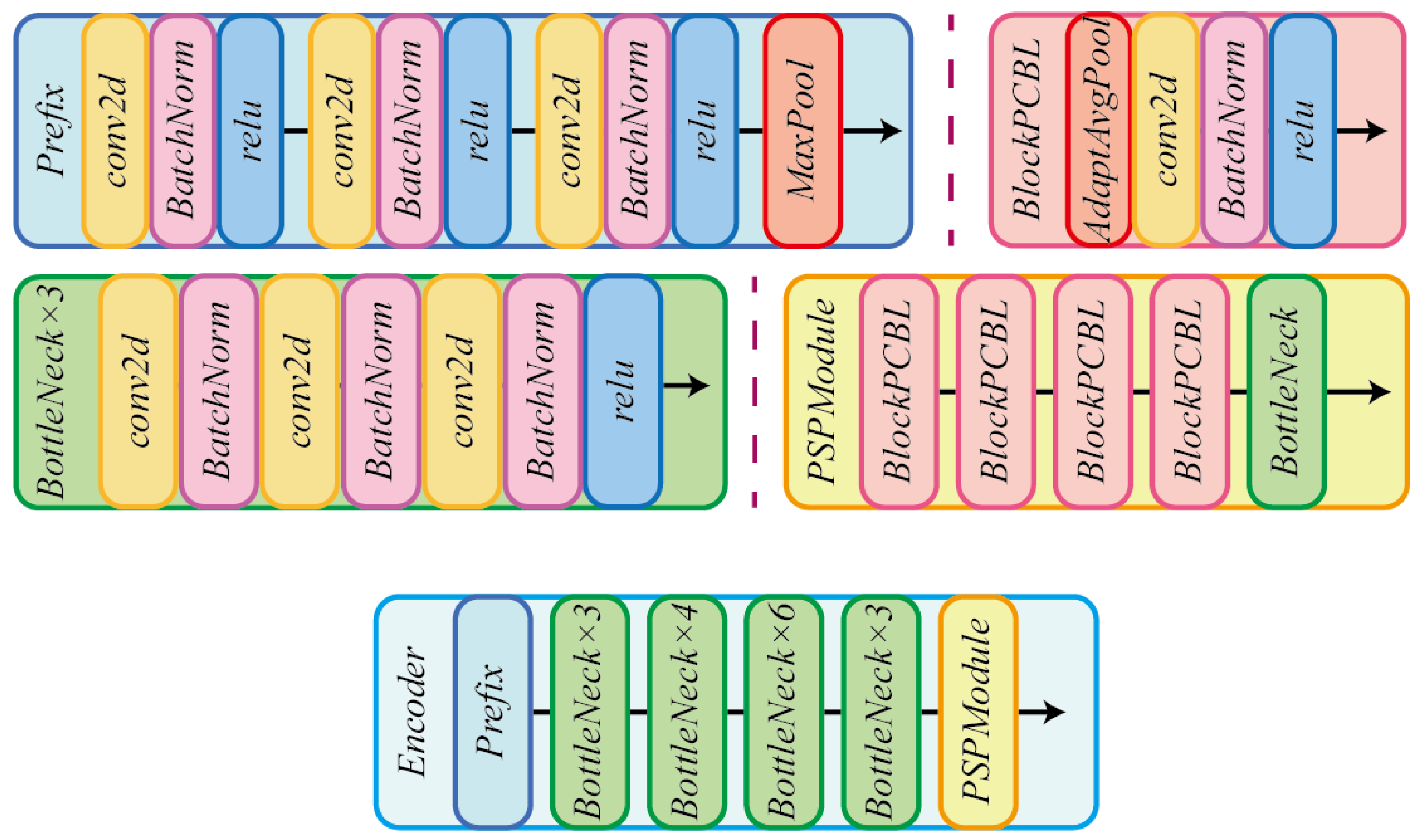
The main-encoder is based on ResNet-50 [
44], with dilated convolutions, followed by one PSP module [
45] for additional enhancements in extracting features. It is a widely used general backbone that has been proven to have good performance in different segmentation tasks. The input of the main-encoder is unperturbed images and it outputs feature maps as the input for the main-decoder. The feature maps concatenate both high-dimensional and low-dimensional features, extracted by residual layers composed of a series of bottleneck blocks, shown in
Figure 3.
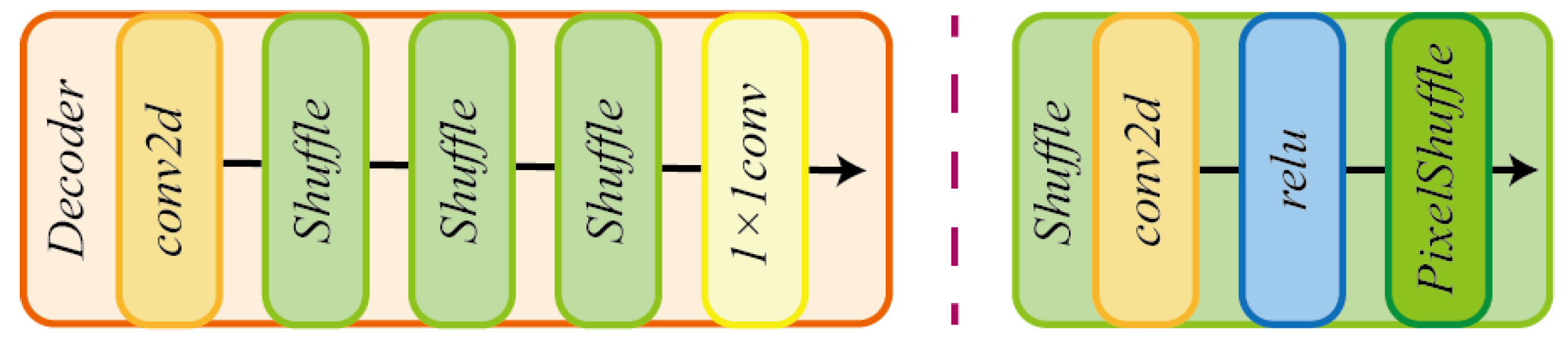
Main Decoder: Feature maps generated from the main-encoder are fed into the main-decoder to predict the semantic segmentation results of the drivable road area. To maximize the robustness of decoding both original and perturbed features from different encoders, after one Conv2d layer, we only employ the simple 1 × 1 2d-convolution and three pixel shuffle modules as the main-decoder, where a pixel shuffle module consists of three layers: Conv2d, ReLU, and PixelShuffle, shown in
Figure 4.
Auxiliary Encoders: Auxiliary encoders consist of several aux-encoders with different perturbations, including VAT, dropout, feature noise, salt noise, color jittering, and lighting perturbations. And there is more than one aux-encoder for each kind of perturbation. It is denoted as , where K is the total number.
Auxiliary Decoders: Auxiliary Decoders are composed of aux-decoders with perturbations including VAT, dropout, feature noise, feature drop, cutout, and masking, which are not exactly consistent with those used in the aux-encoder because of differences in properties during training in different modules. In the same way as aux-encoders, it can be formulated as follows: .
3.4. Loss Functions
The loss function consists of two parts: a supervised part and an unsupervised part, which are computed using cross-entropy and MSE, respectively. The specific calculation of each part is as follows.
3.4.1. Supervised Loss
The input data are in the form of ((, ),()), where is labeled data, y is the corresponding label of , and is indicated as unlabeled data.
Supervised loss is the first stage calculated. It is consistent with normal fully supervised training, where only main modules, namely the main-encoder
and main-decoder
, participate in the prediction
, shown as (
1).
This section may be divided by subheadings. It should provide a concise and precise description of the experimental results, their interpretation, as well as the experimental conclusions that can be drawn.
Cross-entropy (CE) loss is used for this part, which measures the similarity between
and labels
y, shown as (
2).
3.4.2. Unsupervised Loss
The design idea of unsupervised loss is to enable the model to utilize the information of unlabeled data during inference. For the above purposes, unsupervised loss
is designed to consist of two items: loss of aux-encoders
and loss of aux-decoders
.
We first need to generate pseudo labels
corresponding to the input
, shown as (
4).
On completion of that, a copy of
is sent to each aux-encoder
, where one certain perturbation is applied on it, and then transferred to the main-decoder
to make predictions
. This progress can be formulated as below:
As for the unsupervised loss of aux-decoders
, it is processed through the main-encoder
and each aux-decoder
, which is mathematically expressed as follows:
Following obtaining the predictions
for aux-decoders, MSE loss is calculated as follows:
The loss is back-propagated through aux-encoders and the main-decoder, and is back-propagated through aux-decoders and the main-encoder. Thus, both the main-encoder and main-decoder are able to exploit information of unlabeled data during inference.
3.4.3. Total Loss
At the beginning of training, the model, in a fully supervised way, has learned only a very small amount of information from the labeled data, on the basis of which noisy pseudo labels are generated for unsupervised training. Therefore, the weights of the unsupervised loss computed at the initial training are set small and increase with continued training.
The unsupervised weighting parameter
is used to implement the idea above, and increases from 0 to 1 as training progresses. We denote
as
i, the proportion of labeled data as
p, and the total number of images in the training set as
D. Then,
can be expressed as follows:
Total loss
is formulated as follows:
4. Experiment Settings
The experiment settings contain the detailed configuration of implementation, the settings of the datasets, and the calculations of performance metrics.
4.1. Implementation Details
Our code compilation environment for running all experiments is based on the Pytorch 1.13.0 version of Python 3.8 on one Nvidia RTX3090. All training is performed for 150 epochs and the optimizer is SGD. The supervised and unsupervised learning rates are set to 0.01 and 0.001, respectively. In the parameter settings of SGD, weight decay is set to 0.0001, momentum is set to 0.9, and other parameters are kept in their default settings. We use Poly mode in the lr-scheduler with 1.2 of the parameter pow and other parameters are set to default.
4.2. Datasets
Cityscapes: Cityscapes is a large-scale dataset containing multiple cities that supports different vision tasks such as semantic segmentation and instance segmentation. We only use the semantic segmentation dataset part of Cityscapes, which contains a total of 2985 image materials from 18 cities for the training set and 500 images from 3 cities for the validation set. Every image in Cityscapes has a native size of 2048 × 1024 pixels, which is cropped to 513 × 513 pixels in experiments. There are 34 classes in the original semantic segmentation dataset, which are redundant in road segmentation. Therefore, only the road class is retained, and the remaining classes are merged into one non-road class.
CamVid: CamVid, short for The Cambridge-driving Labeled Video Database, is a lightweight semantic segmentation dataset. Compared with the Cityscapes dataset, the images in CamVid have more complex roads, more vehicles, and smaller dimensions, making prediction relatively more difficult. The CamVid dataset contains 701 images, of which 367 images are in the training set, 101 images belong to the validation set, and 223 images are used in the test set. Each image in CamVid is 480 × 360 pixels in size, and it is cropped to 360 × 360 pixels as the input. The CamVid dataset provides 32 ground-truth semantic labels, which are merged into 11 broad categories when used in a semantic segmentation task. In our experiment, only the road class is preserved and the remaining class are integrated to produce road and non-road class labels applicable to drivable area segmentation.
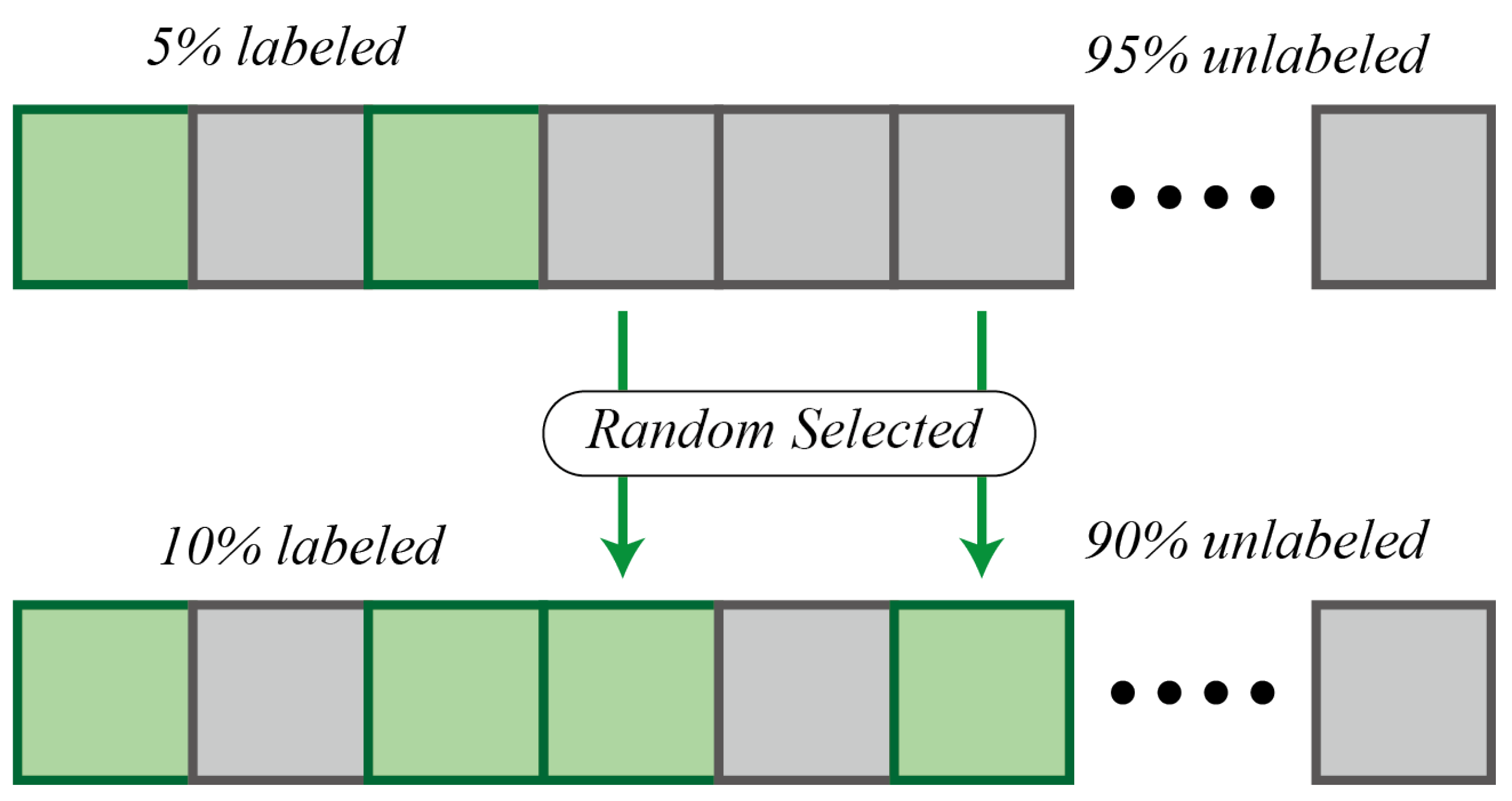
Whether the Cityscapes dataset or the CamVid dataset is used, their data are all labeled data. Thus, in unsupervised training, a certain percentage of images are randomly selected from the original training set, considering them as unlabeled data by ignoring their corresponding labels, and the rest of the data are kept intact for supervised training.
Figure 5 illustrates the above operations.
4.3. Performance Metrics
Given an image for drivable road segmentation, the output of the model will be divided into two classes: “Road” and “Others”. We use five performance metrics to measure the experimental results, which are accuracy, recall, precision, F1-Score, and Intersection over Union (IoU), in all experiments.
4.3.1. Accuracy
Accuracy is used to measure the proportion of pixels with correct predictions in all pixels, which is calculated with (
11).
4.3.2. Recall
The value of recall is the proportion of road class pixels with correct predictions in all road class pixels, which can be expressed as Equation (
12).
4.3.3. Precision
Precision is the proportion of road class pixels with correct predictions in the pixels that are predicted as road pixels, which is calculated with (
13).
4.3.4. F1-Score
The F1-Score is used to measure the average performance of precision and recall, which is calculated with (
14).
4.3.5. IoU
The IoU is used to measure the correlation between road class pixels and the pixels that belong to or are predicted to belong to the road class, which is calculated with (
15).
4.3.6. FPS
FPS is the ratio of the number of images to the total inference time, which measures the real-time performance of the model. The inference time for each batch of test image is denoted as
, and the number of the test dataloader is denoted as
N. Then, the FPS calculation formula is (
16).
5. Experimental Results
5.1. Ablation Studies
The purpose of this experiment is to study the performance of different modules in the models and prove the improvement in our methods. We conducted the following experiments on arrangements with auxiliary modules:
Only aux-encoders (Aux-En).
Only aux-decoders (Aux-De).
Add both aux-encoders and aux-decoders.
Fully supervised model.
In consideration of the rigor of the experiment, we ensured that each semi-supervised model had the same number of auxiliary modules. To be specific, the model with only aux-encoders adds two aux-encoders of each type, comprising twelve in total. And two aux-encoders of each type were appended to the model with only aux-decoders, keeping the totals consistent with the former. As for the model using both aux-encoders and aux-decoders, six aux-encoders and six aux-decoders of each perturbation were employed. In the process of training, 40% images were selected as labeled data, and the results are shown in
Table 2.
Table 2 presents that all semi-supervised methods outperformed the results of fully supervised training. As for semi-supervised methods, the performances of the model with only aux-encoders and the one with only aux-decoders (CCT-structure method) are similar, but the model using both aux-encoders and aux-decoders has significant performance improvement in terms of IoU on two datasets, reaching 0.871 and 0.865, respectively. This illustrates that the synthetic multiple auxiliary modules can make more accurate predictions in different datasets.
5.1.1. Perturbations
The purpose of this experiment is to assess the effectiveness of each kind of perturbation used in aux-encoders. The structure of the aux-decoders remained unchanged during the experiments. In each experiment, one set of aux-encoders consists of six aux-encoders with the same perturbation. And each kind of perturbation was tested in turn on two datasets, both with 40% labeled data. Moreover, we additionally conducted experiments on the model that comprises all kinds of perturbations as comparisons, which is denoted as “All” in
Table 3 and
Table 4. The results are shown below.
It can be seen from the tables above that although the effect of each kind of perturbation may fluctuate on different datasets, they all make improvements compared to the models with only aux-decoders. Methods “All” outperform the rest of them on both datasets, proving that all perturbations are effective and that using multiple perturbations at the same time can improve performance.
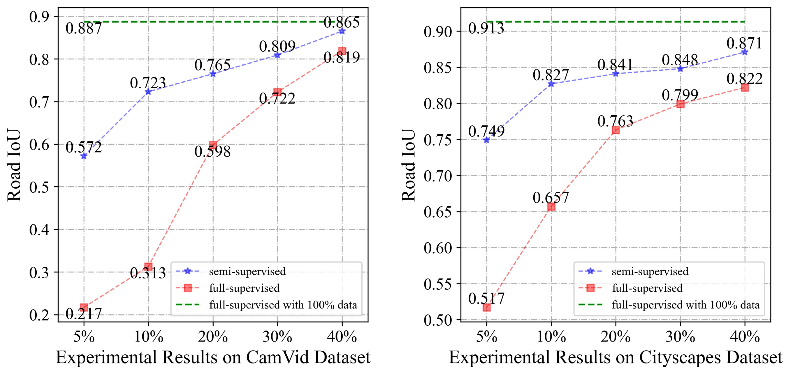
5.1.2. Proportions of Labeled Data
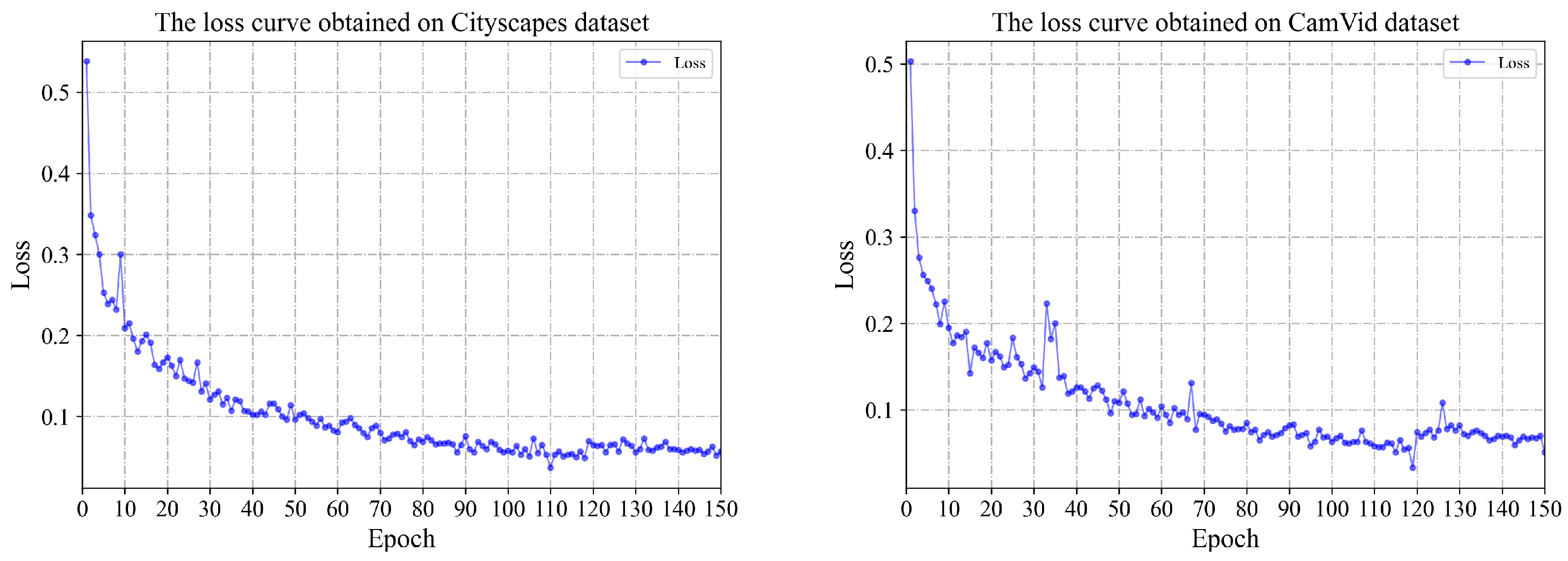
This part of the experiment is designed to analyze the improvements caused by increasing the proportion of labeled data and find a ratio that balances data volume and accuracy. Specifically, the percentage of labeled data is gradually expanded, beginning with 5%, and increasing to 10%, 20%, and finally 40%, which guarantees an inclusion logic in spite of expanding proportions of labeled data, and minimizes the impact of data diversity caused by appending new labeled data. Moreover, in order to investigate convergence during training on two datasets, the loss curves with 40% labeled data are recorded in
Figure 6.
After setting the proportion of labeled data in the semi-supervised datasets, the following two experiments were conducted: fully supervised training on the labeled subset of the semi-supervised datasets and semi-supervised training on the whole of the semi-supervised datasets. All models use the same number of aux-encoders and aux-decoders, and the baseline is the result of fully supervised training on the original datasets with 100% of the data labeled.
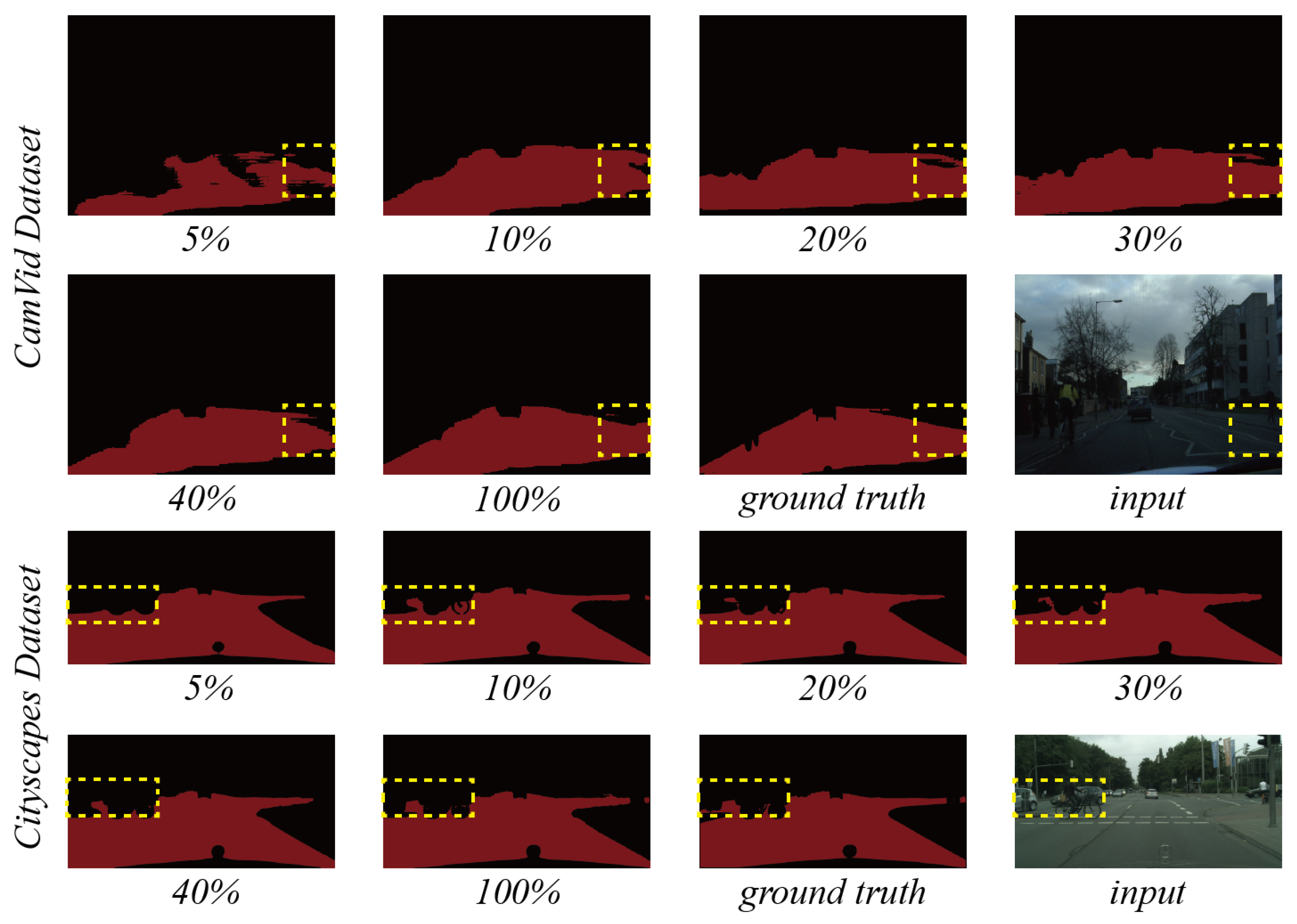
Figure 7 displays the line charts of the relationship between proportions of labeled data and IoU on two datasets and
Figure 8 shows the corresponding visualization of the predictions by semi-supervised models on a certain input. It can be seen from
Figure 7 that there is a significant gap between the IoU of fully supervised and semi-supervised methods when the proportions of labeled data are lower than 20%. With over 40% labeled data, no significant reduction in IoU in semi-supervised training is found compared with the baseline. For example, on the CamVid dataset, the IoU difference between 40% labeled semi-supervised models and fully supervised ones is only 0.022.
In
Figure 6, it can be observed that on both datasets the models have approximate convergence after the 110th epoch. Loss has more fluctuations on CamVid than on Cityscapes because that the latter has a larger numbers and sizes of images than the former.
And in
Figure 8, it is apparent that using 40% labeled data can obtain the same performance as the fully-supervised method on two datasets, and both of them are quite close to the ground truth, especially in the yellow dotted boxes.
In general, therefore, our models with only 40% labeled data can be used as an alternative to fully supervised models when the amount of labeled data is not sufficient.
5.2. Comparison for Other Semi-Supervised Methods
We compared our semi-supervised methods with others in the field of drivable road area segmentation. The experiments were conducted with the same percentage of labeled data (40%) on the Cityscapes and CamVid datasets, which are demonstrated in
Table 5 and
Table 6, respectively. The results of two the datasets are visualized in
Figure 9 and
Figure 10.
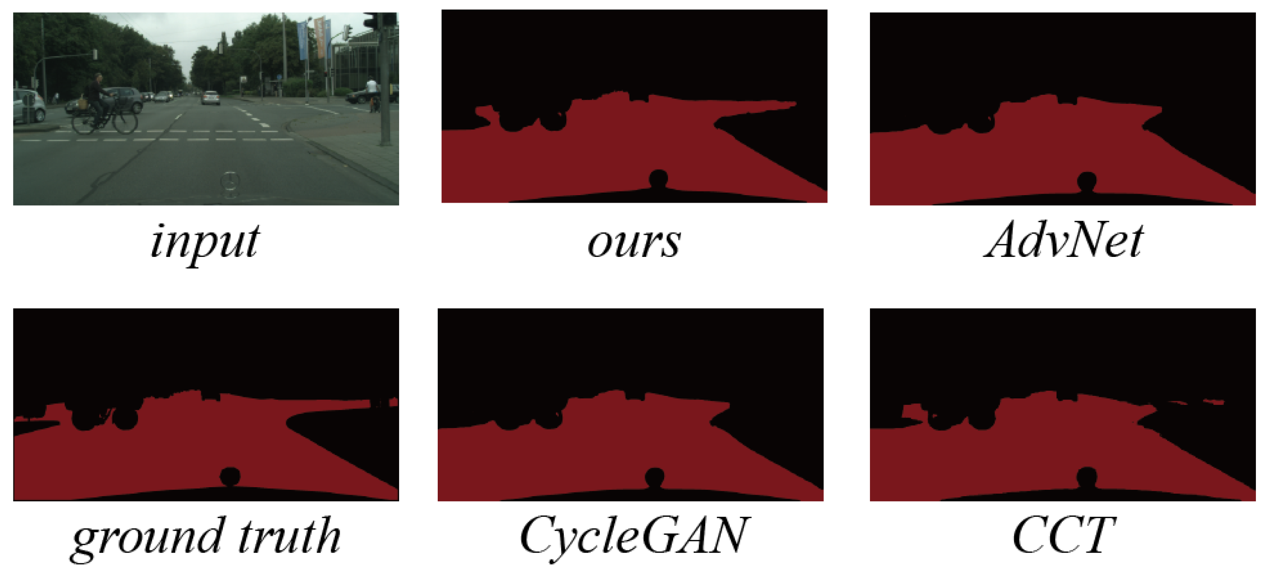
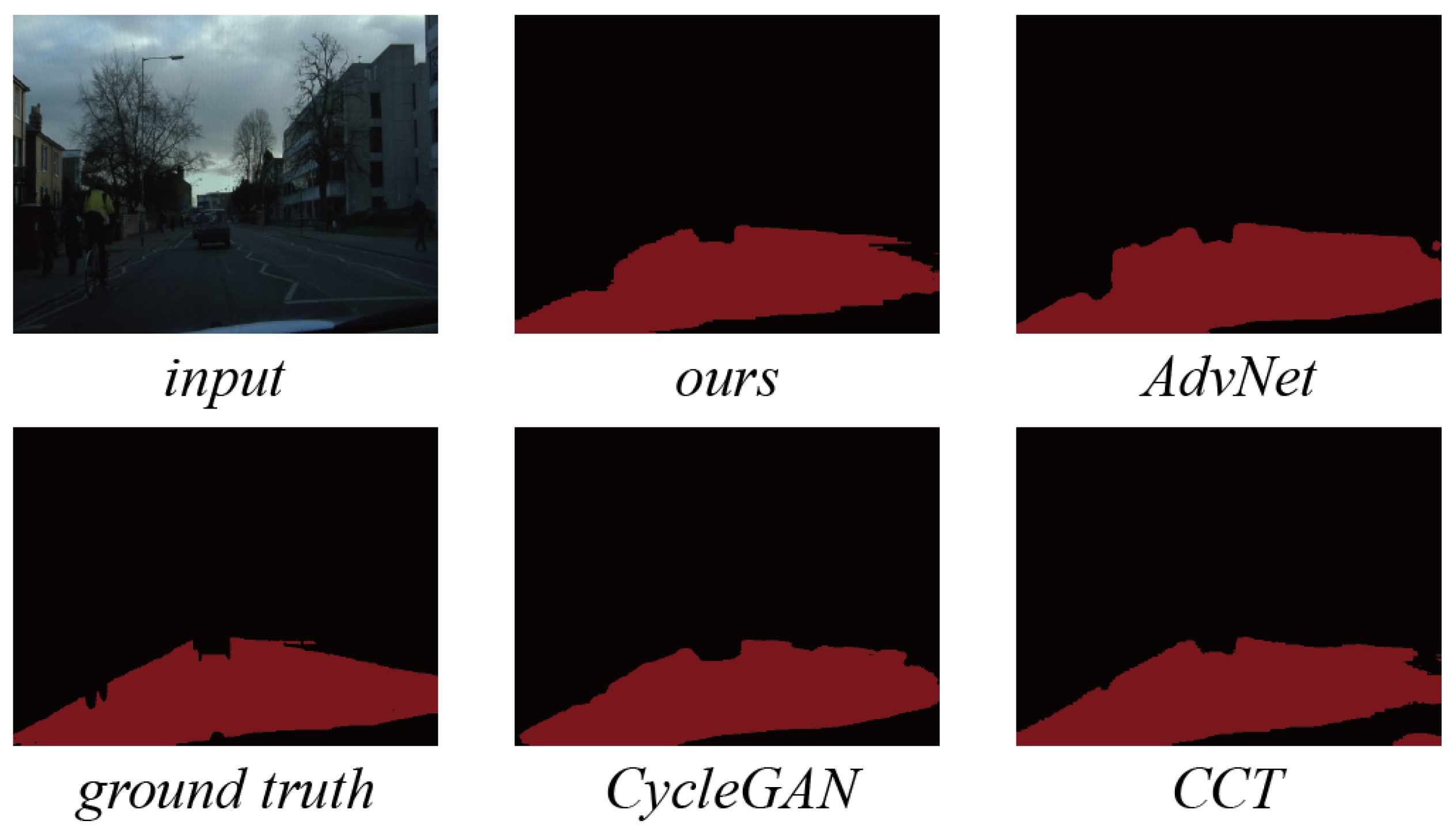
As can be seen from the two tables, our methods outperform the others. On the CamVid dataset, our method achieves the best results. Moreover, on the Cityscapes dataset, the IoU values of our method are significantly better than the second-best method. This is because our methods are based on feature consistency, and we expand the range of feature consistency to cover both the input level and the feature level, which are larger than the feature consistency used by CCT. Therefore, all modules in the inference backbone network of our methods are able to utilize the information of unlabeled data, achieving better performance.
It is also notable that our methods have the highest FPS, which means that our methods are more suitable in real-world autonomous driving scenarios to meet real-time requirements. Therefore, it is concluded that our proposed semi-supervised methods have the best performance in both accuracy and real-time metrics in the field of drivable area segmentation.
6. Discussion
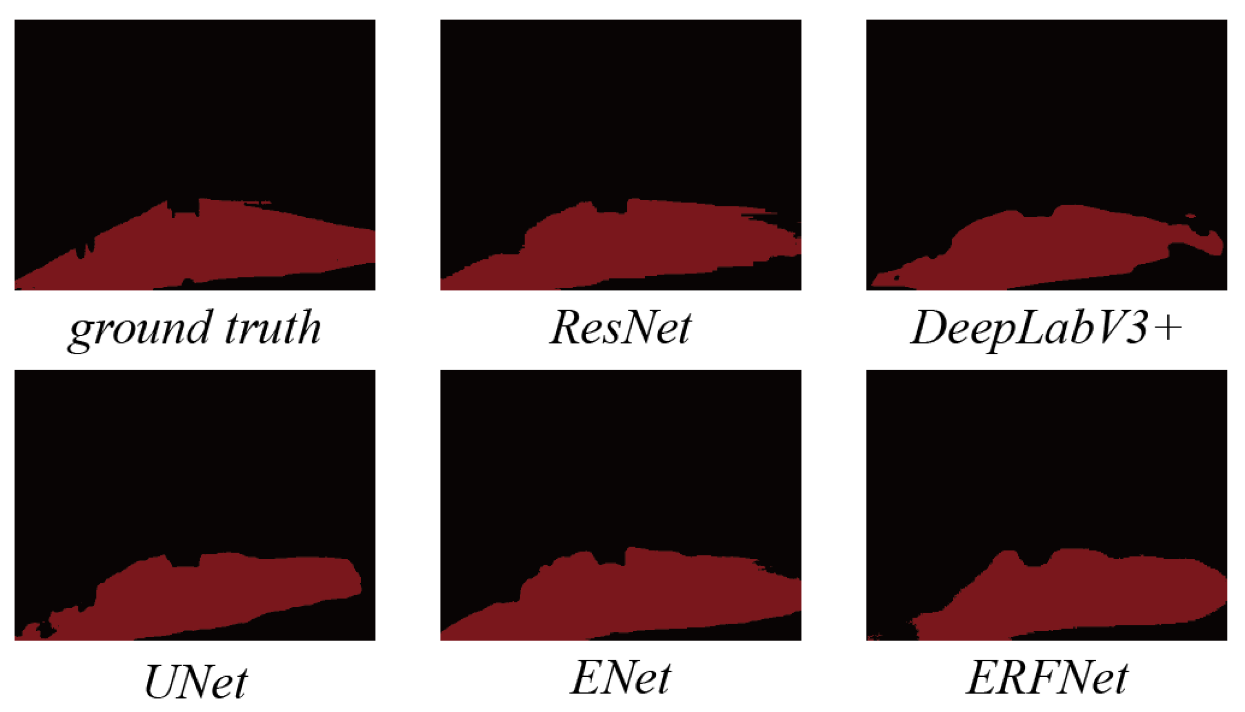
To verify the generalizability and extensibility of our semi-supervised method, we added auxiliary modules in the same way that our semi-supervised methods do on different basic segmentation models and ensured that the perturbed predictions is consistent with the originals. The classical semantic segmentation models that we selected included UNet [
46], ENet [
47], ERFNet [
48], and DeepLabV3+ [
49]. And the experiments were conducted on the CamVid dataset. During semi-supervised training, the proportion of labeled data was set to 40%, indicated by “semi” in
Table 7. Fully supervised experiments were performed on both 40% and 100% of total data for comparison, which are represented by “full” below the different percentages of data in the header of
Table 7. The results are shown in
Table 7 and
Figure 11.
As we can see from
Table 7, when only 40% of the labeled data are used for semi-supervised and fully supervised training, the results of the semi-supervised methods are all significantly improved over the fully supervised one for all basic models. Compared with the results of supervised training using all the data, it can be seen that there is still a gap between the semi-supervised methods and the fully supervised methods, but the gap is marginal, especially on the DeepLabV3+ model. This indicates the generalizability and potential of our methods. With more segmentation models being proposed, employing more advanced networks in our semi-supervised methods could achieve better performance, which is one of the focuses of future work.
7. Conclusions and Future Work
In summary, we proposed novel semi-supervised methods for drivable road segmentation. Our method reaches a good performance by enforcing cross-consistency between the perturbed expanding features and pseudo labels so that they can leverage the information of unlabeled data. Our methods can almost reach the same accuracy and IoU values by only using 40% labeled data as fully supervised methods do with 100% labeled data. Furthermore, the experimental results demonstrate that compared to other semi-supervised methods, ours has better accuracy and real-time performance in the field of drivable area segmentation. Moreover, our methods remain effective when employing other networks, which illustrates the generalizability of our method.
In the future, we will improve our methods by investigating new encoder–decoder-structured backbones that could reach the same IoU with fewer labeled data. If possible, we will deploy the model to an edge computing device such as Nvdia TX2 and perform experiments on real scenario and noisy data. In addition, experimentation regarding where perturbations are placed will be an appealing idea in models with a non-encoder–decoder structure, which can broaden the scope of applications of our semi-supervised method. Moreover, the main module should be as brief as possible to ensure real-time prediction. Finally, designing more efficient perturbations is also one of the focuses of future work.
Author Contributions
Conceptualization, S.M. and C.S.; methodology, S.M.; software, S.M.; validation, S.M.; formal analysis, S.M.; investigation, C.S.; resources, C.S.; data curation, S.M.; writing—original draft preparation, S.M.; writing—review and editing, C.S.; visualization, S.M.; supervision, C.S.; project administration, C.S.; funding acquisition, C.S. All authors have read and agreed to the published version of the manuscript.
Funding
This research received no external funding.
Institutional Review Board Statement
Not applicable.
Informed Consent Statement
Not applicable.
Data Availability Statement
The authors used the publicly available datasets Cityscapes and CamVid for the experiments. The Cityscapes dataset is available in [
50]. The CamVid dataset is available in [
51].
Conflicts of Interest
The authors declare no conflict of interest.
References
- Yurtsever, E.; Lambert, J.; Carballo, A.; Takeda, K. A Survey of Autonomous Driving: Common Practices and Emerging Technologies. IEEE Access 2020, 8, 58443–58469. [Google Scholar] [CrossRef]
- Wen, L.-H.; Jo, K.-H. Deep Learning-Based Perception Systems for Autonomous Driving: A Comprehensive Survey. Neurocomputing 2022, 489, 255–270. [Google Scholar] [CrossRef]
- Bar Hillel, A.; Lerner, R.; Levi, D.; Raz, G. Recent Progress in Road and Lane Detection: A Survey. Mach. Vis. Appl. 2014, 25, 727–745. [Google Scholar] [CrossRef]
- Yao, J.; Ramalingam, S.; Taguchi, Y.; Miki, Y.; Urtasun, R. Estimating Drivable Collision-Free Space from Monocular Video. In Proceedings of the 2015 IEEE Winter Conference on Applications of Computer Vision, Waikoloa, HI, USA, 5–9 January 2015; pp. 420–427. [Google Scholar]
- Yu, F.; Xiu, X.; Li, Y. A Survey on Deep Transfer Learning and Beyond. Mathematics 2022, 10, 3619. [Google Scholar] [CrossRef]
- Jaiswal, A.; Babu, A.R.; Zadeh, M.Z.; Banerjee, D.; Makedon, F. A Survey on Contrastive Self-Supervised Learning. Technologies 2020, 9, 2. [Google Scholar] [CrossRef]
- Ericsson, L.; Gouk, H.; Loy, C.C.; Hospedales, T.M. Self-Supervised Representation Learning: Introduction, advances, and challenges. IEEE Signal Process. Mag. 2022, 39, 42–62. [Google Scholar] [CrossRef]
- Yang, X.; Song, Z.; King, I.; Xu, Z. A Survey on Deep Semi-Supervised Learning. IEEE Trans. Knowl. Data Eng. 2023, 35, 8934–8954. [Google Scholar] [CrossRef]
- Gao, Y.; Song, Y.; Yang, Z. A Real-Time Drivable Road Detection Algorithm in Urban Traffic Environment. In Computer Vision and Graphics; Bolc, L., Tadeusiewicz, R., Chmielewski, L.J., Wojciechowski, K., Eds.; Lecture Notes in Computer Science; Springer: Berlin/Heidelberg, Germany, 2012; Volume 7594, pp. 387–396. ISBN 978-3-642-33563-1. [Google Scholar]
- Graovac, S.; Goma, A. Detection of Road Image Borders Based on Texture Classification. Int. J. Adv. Robot. Syst. 2012, 9, 242. [Google Scholar] [CrossRef]
- Alvarez, J.M.Á.; Lopez, A.M. Road Detection Based on Illuminant Invariance. IEEE Trans. Intell. Transport. Syst. 2011, 12, 184–193. [Google Scholar] [CrossRef]
- Kong, H.; Audibert, J.-Y.; Ponce, J. Vanishing Point Detection for Road Detection. In Proceedings of the 2009 IEEE Conference on Computer Vision and Pattern Recognition, Miami, FL, USA, 20–25 June 2009; pp. 96–103. [Google Scholar]
- Zhou, S.; Gong, J.; Xiong, G.; Chen, H.; Iagnemma, K. Road Detection Using Support Vector Machine Based on Online Learning and Evaluation. In Proceedings of the 2010 IEEE Intelligent Vehicles Symposium, La Jolla, CA, USA, 21–24 June 2010; pp. 256–261. [Google Scholar]
- Foedisch, M.; Takeuchi, A. Adaptive Real-Time Road Detection Using Neural Networks. In Proceedings of the 7th International IEEE Conference on Intelligent Transportation Systems (IEEE Cat. No.04TH8749), Washington, WA, USA, 3–6 October 2004; pp. 167–172. [Google Scholar]
- Crisman, J.D.; Thorpe, C.E. UNSCARF—A Color Vision System for the Detection of Unstructured Roads. In Proceedings of the 1991 IEEE International Conference on Robotics and Automation, Sacramento, CA, USA, 9–11 April 1991; pp. 2496–2501. [Google Scholar]
- Yun, S.; Guo-ying, Z.; Yong, Y. A Road Detection Algorithm by Boosting Using Feature Combination. In Proceedings of the 2007 IEEE Intelligent Vehicles Symposium, Istanbul, Turkey, 13–15 June 2007; pp. 364–368. [Google Scholar]
- Shelhamer, E.; Long, J.; Darrell, T. Fully Convolutional Networks for Semantic Segmentation. IEEE Trans. Pattern Anal. Mach. Intell. 2017, 39, 640–651. [Google Scholar] [CrossRef]
- Badrinarayanan, V.; Kendall, A.; Cipolla, R. SegNet: A Deep Convolutional Encoder-Decoder Architecture for Image Segmentation. IEEE Trans. Pattern Anal. Mach. Intell. 2017, 39, 2481–2495. [Google Scholar] [CrossRef] [PubMed]
- Chen, L.-C.; Papandreou, G.; Kokkinos, I.; Murphy, K.; Yuille, A.L. DeepLab: Semantic Image Segmentation with Deep Convolutional Nets, Atrous Convolution, and Fully Connected CRFs. IEEE Trans. Pattern Anal. Mach. Intell. 2018, 40, 834–848. [Google Scholar] [CrossRef] [PubMed]
- Chen, L.-C.; Papandreou, G.; Schroff, F.; Adam, H. Rethinking Atrous Convolution for Semantic Image Segmentation. arXiv 2017, arXiv:1706.05587. [Google Scholar]
- Krizhevsky, A.; Sutskever, I.; Hinton, G.E. ImageNet Classification with Deep Convolutional Neural Networks. Commun. ACM 2017, 60, 84–90. [Google Scholar] [CrossRef]
- Holder, C.J.; Breckon, T.P.; Wei, X. From On-Road to Off: Transfer Learning within a Deep Convolutional Neural Network for Segmentation and Classification of Off-Road Scenes. In Computer Vision—ECCV 2016 Workshops; Hua, G., Jégou, H., Eds.; Lecture Notes in Computer Science; Springer International Publishing: Cham, Switzerland, 2016; Volume 9913, pp. 149–162. ISBN 978-3-319-46603-3. [Google Scholar]
- Oliveira, G.L.; Burgard, W.; Brox, T. Efficient Deep Models for Monocular Road Segmentation. In Proceedings of the 2016 IEEE/RSJ International Conference on Intelligent Robots and Systems (IROS), Daejeon, Republic of Korea, 9–14 October 2016; pp. 4885–4891. [Google Scholar]
- Reis, F.A.L.; Almeida, R.; Kijak, E.; Malinowski, S.; Guimaraes, S.J.F.; Do Patrocinio, Z.K.G. Combining Convolutional Side-Outputs for Road Image Segmentation. In Proceedings of the 2019 International Joint Conference on Neural Networks (IJCNN), Budapest, Hungary, 14–19 July 2019; pp. 1–8. [Google Scholar]
- Wang, Q.; Gao, J.; Yuan, Y. Embedding Structured Contour and Location Prior in Siamesed Fully Convolutional Networks for Road Detection. IEEE Trans. Intell. Transport. Syst. 2018, 19, 230–241. [Google Scholar] [CrossRef]
- Sun, J.-Y.; Kim, S.-W.; Lee, S.-W.; Kim, Y.-W.; Ko, S.-J. Reverse and Boundary Attention Network for Road Segmentation. In Proceedings of the 2019 IEEE/CVF International Conference on Computer Vision Workshop (ICCVW), Seoul, Republic of Korea, 27–28 October 2019; pp. 876–885. [Google Scholar]
- Lyu, Y.; Bai, L.; Huang, X. Road Segmentation Using CNN and Distributed LSTM. In Proceedings of the 2019 IEEE International Symposium on Circuits and Systems (ISCAS), Sapporo, Japan, 26–29 May 2019; pp. 1–5. [Google Scholar] [CrossRef]
- Scheck, T.; Mallandur, A.; Wiede, C.; Hirtz, G. Where to Drive: Free Space Detection with One Fisheye Camera. In Proceedings of the Twelfth International Conference on Machine Vision (ICMV 2019), Amsterdam, The Netherlands, 31 January 2020; p. 12. [Google Scholar]
- Gong, S.; Zhou, H.; Xue, F.; Fang, C.; Li, Y.; Zhou, Y. FastRoadSeg: Fast Monocular Road Segmentation Network. IEEE Trans. Intell. Transport. Syst. 2022, 23, 21505–21514. [Google Scholar] [CrossRef]
- Jiang, P.; Ergu, D.; Liu, F.; Cai, Y.; Ma, B. A Review of Yolo Algorithm Developments. Procedia Comput. Sci. 2022, 199, 1066–1073. [Google Scholar] [CrossRef]
- Wu, D.; Liao, M.; Zhang, W.; Wang, X.; Bai, X.; Cheng, W.; Liu, W. YOLOP: You Only Look Once for Panoptic Driving Perception. Mach. Intell. Res. 2022, 19, 550–562. [Google Scholar] [CrossRef]
- Han, C.; Zhao, Q.; Zhang, S.; Chen, Y.; Zhang, Z.; Yuan, J. Yolopv2: Better, faster, stronger for panoptic driving perception. arXiv 2022, arXiv:2208.11434. [Google Scholar]
- Qian, Y.; Dolan, J.M.; Yang, M. DLT-Net: Joint detection of drivable areas, lane lines, and traffic object. IEEE Trans. Intell. Transp. Syst. 2020, 21, 4670–4679. [Google Scholar] [CrossRef]
- Vu, D.; Ngo, B.; Phan, H. Hybridnets: End-to-end perception network. arXiv 2022, arXiv:2203.09035. [Google Scholar]
- Shao, M.-E.; Haq, M.A.; Gao, D.-Q.; Chondro, P.; Ruan, S.-J. Semantic segmentation for free space and lane based on grid-based interest point detection. IEEE Trans. Intell. Transp. Syst. 2022, 23, 8498–8512. [Google Scholar] [CrossRef]
- Zhang, Z.; Qin, J.; Wang, S.; Kang, Y.; Liu, Q. ULODNet: A Unified Lane and Obstacle Detection Network Towards Drivable Area Understanding in Autonomous Navigation. J. Intell. Robot. Syst. 2022, 105, 4. [Google Scholar] [CrossRef]
- Kim, S.; Kim, D.; Kim, H. Texture Learning Domain Randomization for Domain Generalized Segmentation. arXiv 2023, arXiv:2303.11546. [Google Scholar]
- Ouali, Y.; Hudelot, C.; Tami, M. Semi-Supervised Semantic Segmentation With Cross-Consistency Training. In Proceedings of the 2020 IEEE/CVF Conference on Computer Vision and Pattern Recognition (CVPR), Seattle, WA, USA, 13–19 June 2020; pp. 12671–12681. [Google Scholar]
- Chen, X.; Yuan, Y.; Zeng, G.; Wang, J. Semi-Supervised Semantic Segmentation with Cross Pseudo Supervision. In Proceedings of the 2021 IEEE/CVF Conference on Computer Vision and Pattern Recognition (CVPR), Nashville, TN, USA, 20–25 June 2021; pp. 2613–2622. [Google Scholar]
- French, G.; Laine, S.; Aila, T.; Mackiewicz, M.; Finlayson, G. Semi-Supervised Semantic Segmentation Needs Strong, Varied Perturbations. arXiv 2020, arXiv:1906.01916. [Google Scholar]
- Olsson, V.; Tranheden, W.; Pinto, J.; Svensson, L. ClassMix: Segmentation-Based Data Augmentation for Semi-Supervised Learning. In Proceedings of the 2021 IEEE Winter Conference on Applications of Computer Vision (WACV), Waikoloa, HI, USA, 3–8 January 2021; pp. 1368–1377. [Google Scholar] [CrossRef]
- Miyato, T.; Maeda, S.; Koyama, M.; Ishii, S. Virtual Adversarial Training: A Regularization Method for Supervised and Semi-Supervised Learning. IEEE Trans. Pattern Anal. Mach. Intell. 2019, 41, 1979–1993. [Google Scholar] [CrossRef]
- Oliva, A.; Torralba, A. The Role of Context in Object Recognition. Trends Cogn. Sci. 2007, 11, 520–527. [Google Scholar] [CrossRef]
- He, K.; Zhang, X.; Ren, S.; Sun, J. Deep Residual Learning for Image Recognition. In Proceedings of the 2016 IEEE Conference on Computer Vision and Pattern Recognition (CVPR), Las Vegas, NV, USA, 27–30 June 2016; pp. 770–778. [Google Scholar]
- Zhao, H.; Shi, J.; Qi, X.; Wang, X.; Jia, J. Pyramid Scene Parsing Network. In Proceedings of the 2017 IEEE Conference on Computer Vision and Pattern Recognition (CVPR), Honolulu, HI, USA, 21–26 July 2017; pp. 6230–6239. [Google Scholar] [CrossRef]
- Ronneberger, O.; Fischer, P.; Brox, T. U-Net: Convolutional Networks for Biomedical Image Segmentation. arXiv 2015, arXiv:1505.04597. [Google Scholar]
- Paszke, A.; Chaurasia, A.; Kim, S.; Culurciello, E. ENet: A Deep Neural Network Architecture for Real-Time Semantic Segmentation. arXiv 2016, arXiv:1606.02147. [Google Scholar]
- Romera, E.; Alvarez, J.M.; Bergasa, L.M.; Arroyo, R. Efficient ConvNet for Real-Time Semantic Segmentation. In Proceedings of the 2017 IEEE Intelligent Vehicles Symposium (IV), Los Angeles, CA, USA, 11–14 June 2017; pp. 1789–1794. [Google Scholar]
- Chen, L.-C.; Zhu, Y.; Papandreou, G.; Schroff, F.; Adam, H. Encoder-Decoder with Atrous Separable Convolution for Semantic Image Segmentation. arXiv 2018, arXiv:1802.02611. [Google Scholar]
- Cordts, M.; Omran, M.; Ramos, S.; Rehfeld, T.; Enzweiler, M.; Benenson, R.; Franke, U.; Roth, S.; Schiele, B. The Cityscapes Dataset for Semantic Urban Scene Understanding. In Proceedings of the 2016 IEEE Conference on Computer Vision and Pattern Recognition (CVPR), Las Vegas, NV, USA, 27–30 June 2016; pp. 3213–3223. [Google Scholar] [CrossRef]
- Brostow, G.J.; Fauqueur, J.; Cipolla, R. Semantic Object Classes in Video: A High-Definition Ground Truth Database. Pattern Recognit. Lett. 2009, 30, 88–97. [Google Scholar] [CrossRef]
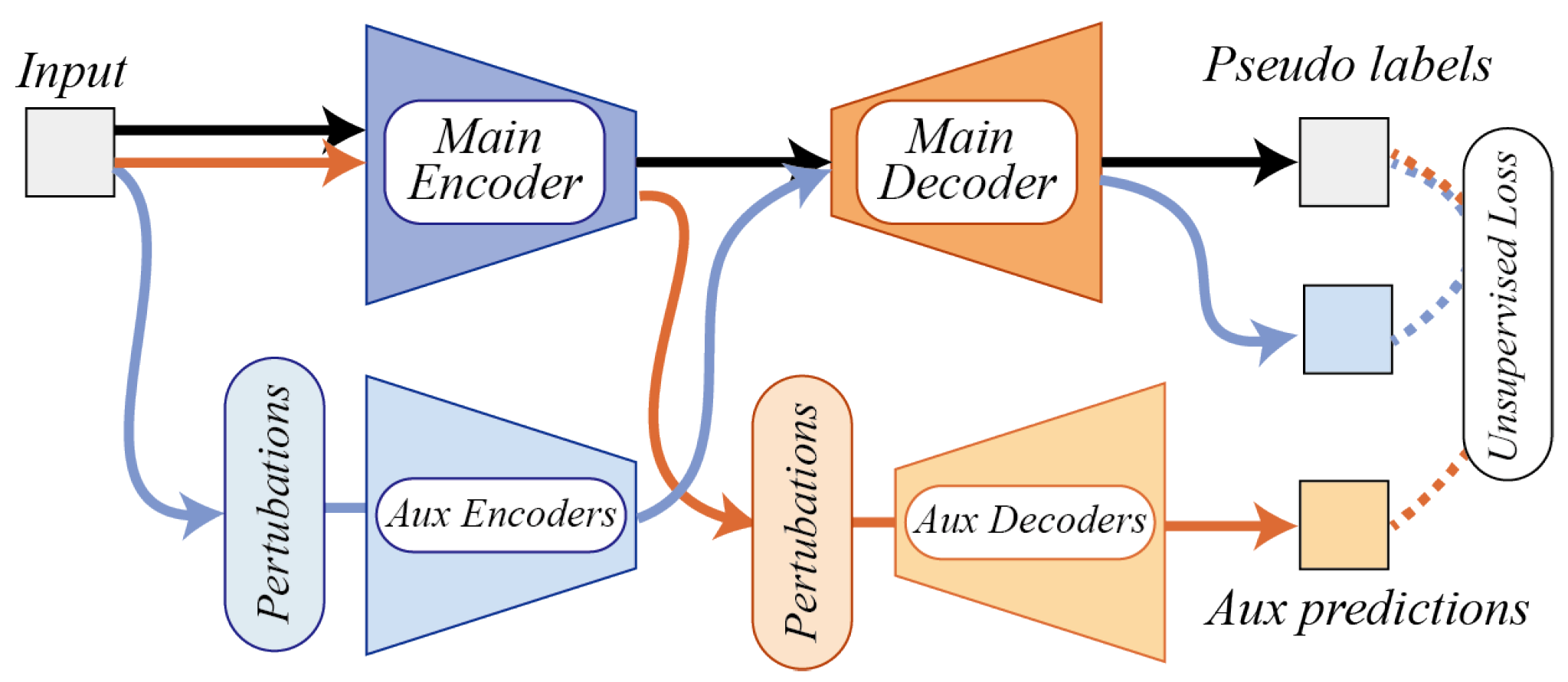
Figure 1.
The overall flow of semi-supervised training: Main modules first generate pseudo labels on original unlabeled data, which is shown in black arrows. Then, auxiliary modules make predictions on perturbed data, and unsupervised loss is designed to measure the discrepancy between pseudo labels and perturbed prediction, which are shown in light blue arrows (predictions perturbed by auxiliary encoders) and orange arrows (predictions perturbed by auxiliary decoders).
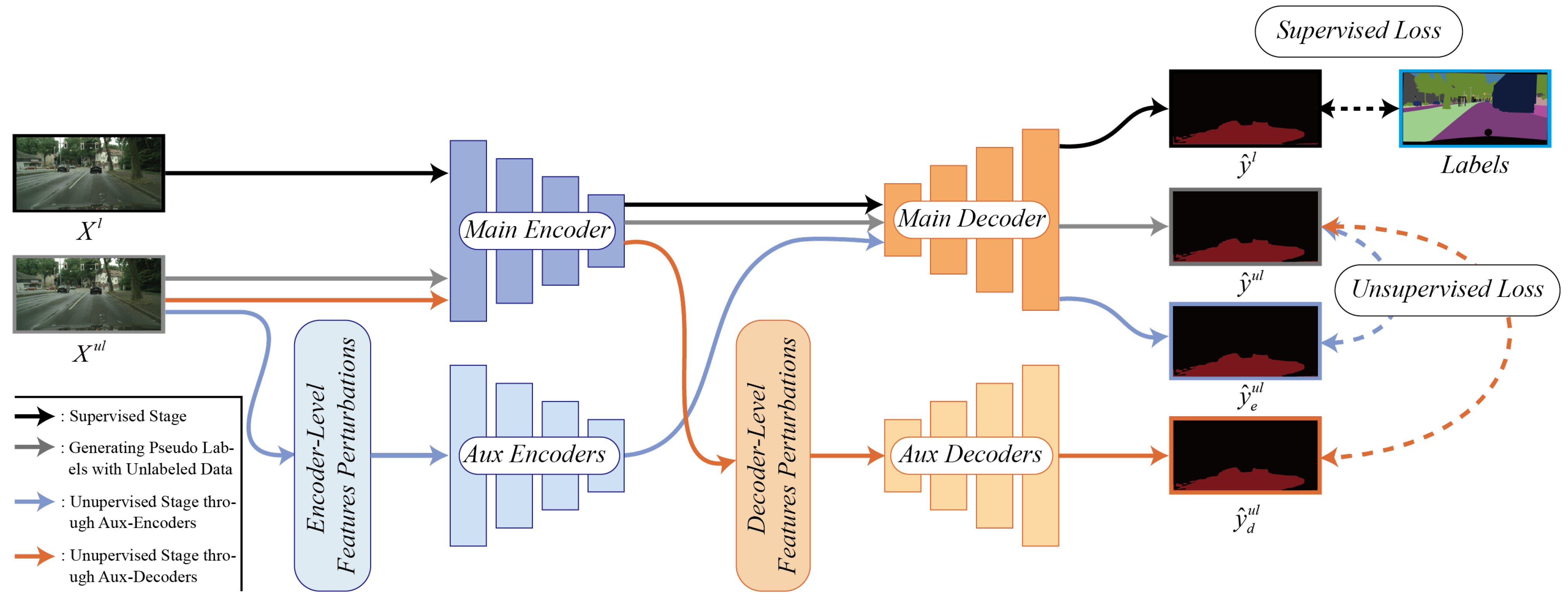
Figure 2.
The overall algorithm can be divided into four stages. Stage 1: supervised training is illustrated as black lines. Stage 2: the predictions on unlabeled data are used to ensure consistency between the perturbed prediction yielded from stages 3 and 4 by MSE loss, shown as gray lines. Stage 3: unlabeled data are reconstructed by aux-encoders generating perturbed tensors, and then those tensor are transferred to main decoder for prediction, shown as light blue lines. Stage 4: main encoder transforms the unlabeled data into feature maps and then distributes them to aux-decoders with different perturbations to make the prediction.
Figure 3.
The detailed structures of the main-encoder.
Figure 3.
The detailed structures of the main-encoder.
Figure 4.
The detailed structures of the main decoder.
Figure 4.
The detailed structures of the main decoder.
Figure 5.
Randomly selecting some new labeled data and adding them into preceding selected data.
Figure 5.
Randomly selecting some new labeled data and adding them into preceding selected data.
Figure 6.
The loss curves obtained on Cityscapes and CamVid datasets show that the models have approximated convergence after 110th epoch.
Figure 6.
The loss curves obtained on Cityscapes and CamVid datasets show that the models have approximated convergence after 110th epoch.
Figure 7.
With the increment in the labeled data, the IoU values become closer to the baseline. With over 40% labeled data, no significant reduction in IoU in semi-supervised training is found compared with baseline.
Figure 7.
With the increment in the labeled data, the IoU values become closer to the baseline. With over 40% labeled data, no significant reduction in IoU in semi-supervised training is found compared with baseline.
Figure 8.
Prediction of semi-supervised methods on two datasets with different labeled-data percentages.
Figure 8.
Prediction of semi-supervised methods on two datasets with different labeled-data percentages.
Figure 9.
Examples of making predictions on certain images from Cityscapes using our method and others (CycleGAN, AdvNet, and CCT).
Figure 9.
Examples of making predictions on certain images from Cityscapes using our method and others (CycleGAN, AdvNet, and CCT).
Figure 10.
Examples of making predictions on certain images from CamVid using our method and others (CycleGAN, AdvNet, and CCT).
Figure 10.
Examples of making predictions on certain images from CamVid using our method and others (CycleGAN, AdvNet, and CCT).
Figure 11.
Our method can achieve significant improvement when applied to different segmentation models (ResNet, UNet, ENet, ERFNet, and DeepLabV3).
Figure 11.
Our method can achieve significant improvement when applied to different segmentation models (ResNet, UNet, ENet, ERFNet, and DeepLabV3).
Table 1.
Literature review: related works on road area segmentation.
Table 1.
Literature review: related works on road area segmentation.
| Reference | Type | Method/Model |
|---|
| He et al. [9] | Image processing | a color-feature- and edge-image-based method. |
| Graovac et al. [10] | Image processing | a texture-classification-based method. |
| Alvarez et al. [11] | Image processing | an illuminant-invariance-based method. |
| Alvarez et al. [12] | Image processing | a Gabor-filter- and clustering-based vanish point method |
| Zhou et al. [13] | Machine learning | a color-feature- and texture-feature-based SVM method. |
| Yao et al. [4] | Machine learning | a geometric-feature (including edges, color and homography)-based structured SVM method. |
| Foedisch et al. [14] | Machine learning | a color-features-based neural network. |
| Crisman et al. [15] | Machine learning | a edge-based modified clustering method. |
| Yun et al. [16] | Machine learning | a boosting-, SVM-, and random forest-classifier-based complex method |
| Holder et al. [22] | Deep learning | a deep CNN-based model |
| Oliveira et al. [23] | Deep learning | an up-convolutional network-based model. |
| Reis et al. [24] | Deep learning | an all-layer- and stage-layer-module-based model. |
| Wang et al. [25] | Deep learning | a siamese fully convolutional network-based model. |
| Sun et al. [26] | Deep learning | an improved SegNet with reverse attention-based model. |
| Lyu et al. [27] | Deep learning | a CNN- combined with LSTM-based model. |
| Scheck et al. [28] | Deep learning | a ResNet101 v2-based model for fisheye lens. |
| Gong et al. [29] | Deep learning | an asymmetric dilated CNN-based model. |
| Wu et al. [31] | Deep learning: multi-tasking learning | YoloP: a CSPDarkNet-backbone-based multi-task model. |
| Han et al. [32] | Deep learning: multi-tasking learning | YoloPv2: a improved model based on YoloP with an E-ELAN-based shared encoder. |
| Qian et al. [33] | Deep learning: multi-tasking learning | DLT-Net: a model with the improved VGG16-based encoder. |
| Vu et al. [34] | Deep learning: multi-tasking learning | HybridNets: a model with a backbone of EfficientNet-B3. |
| Shao et al. [35] | Deep learning: multi-tasking learning | GBIP-Net: a method focused on interest points whose model is based on SAMT framework. |
| Zhang et al. [36] | Deep learning: multi-tasking learning | ULODNet: a ResNet- or DarkNet-backbone-based network. |
Table 2.
Results on models with different auxiliary modules with 40% labeled data.
Table 2.
Results on models with different auxiliary modules with 40% labeled data.
| Method | Cityscapes | CamVid |
|---|
|
Aux-En
|
Aux-De
|
Accuracy
|
IoU
|
Accuracy
|
IoU
|
|---|
| × | × | 0.931 | 0.825 | 0.915 | 0.822 |
| ✓ | × | 0.952 | 0.857 | 0.930 | 0.824 |
| × | ✓ | 0.951 | 0.845 | 0.934 | 0.836 |
| ✓ | ✓ | 0.954 | 0.871 | 0.939 | 0.865 |
Table 3.
Results on different perturbations of aux-encoders in Camvid dataset with 40% labeled data.
Table 3.
Results on different perturbations of aux-encoders in Camvid dataset with 40% labeled data.
| Method | Accuracy | Recall | Precision | F1-Score | IoU |
|---|
| VAT | 0.919 | 0.907 | 0.975 | 0.938 | 0.832 |
| Dropout | 0.928 | 0.904 | 0.981 | 0.943 | 0.849 |
| Feature noise | 0.932 | 0.924 | 0.975 | 0.948 | 0.848 |
| Salt noise | 0.926 | 0.904 | 0.985 | 0.942 | 0.843 |
| Color jittering | 0.925 | 0.908 | 0.981 | 0.943 | 0.838 |
| Lighting | 0.932 | 0.933 | 0.975 | 0.953 | 0.862 |
| All | 0.939 | 0.931 | 0.977 | 0.953 | 0.865 |
Table 4.
Results on different perturbations of aux-encoders in Cityscapes dataset with 40% labeled data.
Table 4.
Results on different perturbations of aux-encoders in Cityscapes dataset with 40% labeled data.
| Method | Accuracy | Recall | Precision | F1-Score | IoU |
|---|
| VAT | 0.948 | 0.953 | 0.966 | 0.960 | 0.865 |
| Dropout | 0.950 | 0.950 | 0.971 | 0.960 | 0.862 |
| Feature noise | 0.950 | 0.952 | 0.968 | 0.960 | 0.864 |
| Salt noise | 0.952 | 0.955 | 0.967 | 0.961 | 0.857 |
| Color jittering | 0.949 | 0.951 | 0.967 | 0.959 | 0.861 |
| Lighting | 0.953 | 0.956 | 0.968 | 0.963 | 0.868 |
| All | 0.954 | 0.957 | 0.969 | 0.963 | 0.871 |
Table 5.
Performance of different semi-supervised methods on Cityscapes.
Table 5.
Performance of different semi-supervised methods on Cityscapes.
| Method | Accuracy | Recall | Precision | F1-Score | Road IoU | FPS |
|---|
| ours | 0.957 | 0.968 | 0.970 | 0.969 | 0.871 | 106.1 |
| CycleGAN | 0.948 | 0.960 | 0.962 | 0.961 | 0.853 | 88.6 |
| AdvNet | 0.921 | 0.946 | 0.952 | 0.949 | 0.799 | 29.2 |
| CCT | 0.945 | 0.964 | 0.950 | 0.956 | 0.827 | 95.7 |
Table 6.
Performance of different semi-supervised methods on CamVid.
Table 6.
Performance of different semi-supervised methods on CamVid.
| Method | Accuracy | Recall | Precision | F1-Score | Road IoU | FPS |
|---|
| ours | 0.961 | 0.962 | 0.985 | 0.974 | 0.865 | 114.2 |
| CycleGAN | 0.904 | 0.942 | 0.961 | 0.951 | 0.841 | 100.6 |
| AdvNet | 0.941 | 0.953 | 0.967 | 0.960 | 0.789 | 61.8 |
| CCT | 0.959 | 0.948 | 0.989 | 0.968 | 0.861 | 103 |
Table 7.
Performance of different base segmentation models on CamVid.
Table 7.
Performance of different base segmentation models on CamVid.
| Model | Semi (40% Labeled) | Full (40% Labeled) | Full (100% Labeled) | FPS (40% Labeled) |
|---|
| UNet | 0.724 | 0.683 | 0.779 | 82.1 |
| ENet | 0.855 | 0.819 | 0.892 | 71.0 |
| ERFNet | 0.829 | 0.797 | 0.903 | 104.5 |
| DeepLabV3+ | 0.803 | 0.772 | 0.815 | 97.7 |
| Disclaimer/Publisher’s Note: The statements, opinions and data contained in all publications are solely those of the individual author(s) and contributor(s) and not of MDPI and/or the editor(s). MDPI and/or the editor(s) disclaim responsibility for any injury to people or property resulting from any ideas, methods, instructions or products referred to in the content. |
© 2023 by the authors. Licensee MDPI, Basel, Switzerland. This article is an open access article distributed under the terms and conditions of the Creative Commons Attribution (CC BY) license (https://creativecommons.org/licenses/by/4.0/).


