A Novel Method for the Analysis and Optimization of End Face Stress in Cycloidal Gears Based on Conformal Mapping

Featured Application

This research presents a novel method for optimizing stress distribution in gear designs, particularly improving the accuracy of intricate geometries like cycloidal gears.

Abstract

In the realm of precision engineering, the evaluation of stress distributions in complex geometries, such as the end face of gears, is paramount for determining performance characteristics, including the fatigue life of transmission devices. This research introduces a methodology that combines the method of conformal mapping for multiply connected regions with a proposed global scaling factor. This combination facilitates the transformation of stress computations from intricate geometries to a unit circle. By employing this method as a foundation for surrogate models, and by incorporating the Bayesian-enhanced least squares genetic algorithm optimization technique, this study refines the end face stress distribution, particularly considering variations induced by tooth profile modification errors. The results delineate a design parameter domain that is conducive to achieving uniform stress distribution, offering a refined perspective and methodology for the design of cycloidal wheels.

1. Introduction

Stress distribution plays a pivotal role in the design of gear end surfaces [1,2,3], profoundly affecting the gear’s performance and lifespan. Two primary determinants shape this distribution: the applied load and the material properties of the gear. Typically, the loads imposed on gears originate from power sources such as engines or motors on the input shaft. These loads give rise to compressive and shear stresses on the gear, culminating in varied stress distributions. Furthermore, the intrinsic attributes of the gear material, including its strength, hardness, and toughness, further delineate this distribution.

Stress distribution in gears plays a pivotal role in determining their longevity, reliability, and susceptibility to fatigue. When gears are subjected to loads, the distribution of stress can significantly influence their fatigue lives and the associated risk of fracture [4,5,6]. An optimized stress distribution enhances the gear’s lifespan and reduces failure risks. Many studies have emphasized the importance of understanding the underlying failure mechanisms in gear systems to enhance their reliability, efficiency, and longevity, with fatigue failure, particularly contact and bending fatigue, being a recurring concern. Guan and Wang utilized FEA to delve into the stress distribution in high-speed helical gear shafts, pinpointing fatigue fracture as the primary failure mode [7]. Similarly, the research by Qian et al. indicated that the maximum stress location correlates with the failure site [8]. FEA also surfaced as a crucial tool in other studies, such as those by Jalaja et al., which inspected aluminum alloy brake reducers for reusable launch vehicles, and by Yang et al., who explored stress sensitivity and fatigue life in harmonic gear drives. These analyses underlined the necessity to grasp material attributes and grain orientation to foresee ductile overload or fatigue failures [9]. In a contrasting perspective, Yin et al. highlighted the repercussions of misalignment, such as tooth breakage and pitting due to surface contact fatigue [10]. Meanwhile, Tsai et al. concentrated on structural stress analysis techniques and the prediction of fatigue life in high reduction ratio reducers, juxtaposing FEA-derived outcomes with formula-calculated stress and fatigue life estimates [11]. Furthermore, specific fatigue forms, like rolling contact fatigue in RV reducer crankshafts, have been investigated. Li et al. introduced a 3D elasto-plastic contact model, factoring in hardness gradients and initial residual stress for better fatigue life prediction [12]. Additionally, Feng et al. examined the breakdown of a secondary driving helical gear in electric vehicles, linking the failure to elevated contact stress and impact load caused by subpar material properties [13]. Collectively, these studies underscore the multifaceted aspects of gear failures. Addressing fatigue requires a holistic comprehension of stress distribution, material characteristics, and operational conditions. Consequently, the use of advanced analytical tools like FEA becomes indispensable in designing, diagnosing, and refining gear systems across various applications.

Stress distribution in gears profoundly impacts their transmission efficiencies, closely relating to gear friction, wear, and energy losses [14,15]. Optimizing this distribution can lead to improved transmission and energy conversion efficiencies. A surge of research has focused on the interplay between stress and transmission performance in various reducers, aiming to boost efficiency, reliability, and load capacity through innovative mechanical designs and mathematical modeling. Sun and Han’s examination of the China Bearing Reducer (CBR) underscored the significance of the clearance between the cycloid teeth and pin on the contact force and stress [16]. Using finite element methods, Song et al. found that in RV reducers, the eccentric shaft’s stiffness is of greater concern than the material strength [17]. Hsieh and team compared traditional and novel designs for two-stage speed reducers, analyzing their implications for stress and motion [18]. Mo et al. showcased the 2K-H internal meshing abnormal cycloidal gear (ACG) planetary reducer’s superior transmission properties and reduced stress levels [19], while Hsieh proposed a distinctive transmission design that optimized stress distribution [20]. The analytical models by Li et al. and Kim et al. took into account factors like elastic- and heat-induced deformations in cycloid and planetary gear speed reducers [21]. Huang et al.’s focus was on dynamic characteristics, using both static and dynamic finite element analyses to evaluate the stress distribution [22]. Delving into specific applications, Bao et al.’s finite element analysis led to a notable reduction in the contact stress in cycloid gears [23].

Moreover, the acoustic properties of gears are also affected by stress distribution. Fluctuations in stress can alter a gear’s vibration and noise levels, implying that a meticulously crafted stress distribution design can diminish these acoustic interferences, thereby improving the gear’s acoustic performance [24]. In summation, recognizing and addressing stress distribution in gears, especially on their end surfaces, is vital. A competent design that considers this aspect can not only refine the performance and reliability of the gear but also uplift the acoustic attributes, thereby optimizing the overall functionality of the mechanical system.

Despite the extensive research on gear stress distribution, several gaps persist, which our investigation aims to bridge. Firstly, while most of the prevailing studies lean heavily on FEA to interpret stress and fatigue, the wide dimensional span between gear profile modifications and the actual gear geometry poses computational challenges. Mature FEA software, when applied to these scenarios, is computationally intensive, making efficient analysis and optimization elusive. To counteract this, advanced optimization techniques like the Bayesian-enhanced least squares genetic algorithm optimization method (BLSGAOM) emerge as imperative tools, offering precise and cost-effective analyses. Secondly, the assumption of idealized conditions in many studies often overlooks real-world intricacies like input crank deformation, pin tooth runout, and backlash angles. These variables, aside from their individual impacts, can also lead to altered contact characteristics, affecting the overall gear performance. Thirdly, there is a discernible focus on tooth surface contact in the literature, sidelining the more complex yet crucial aspect of stress analysis on gear end surfaces with intricate shapes. This oversight potentially masks a significant area of stress accumulation, which might be the precursor to premature gear failures or sub-optimal performance. In summary, while the field has made commendable strides, a holistic, integrated approach that amalgamates advanced computational methods, real-world variables, and a deep dive into lesser-explored gear regions is the next frontier in gear stress distribution research.

This study is methodically structured to offer a systematic understanding of cycloid gear stress analysis and optimization. Initially, this paper lays the groundwork with a quadratic contact surface analysis and force modeling (Section 2). We then delve into an advanced analysis of end face stress in cycloid gears, introducing a conformal mapping technique that is suitable for multiply connected domains and discussing the geometric intricacies of cycloid gear profiles with pores (Section 3.1 and Section 3.2). The novel SACGES-CMMD method is presented (Section 3.3), followed by insights into the global stress scaling factor (Section 3.4). Section 4 propounds an innovative optimization approach, integrating Bayesian analysis with a genetic algorithm. Comprehensive results, ranging from the impact of clearance on contact force fluctuations to a comparative analysis of SACGES-CMMD versus conventional FEM, are detailed in Section 5. This study culminates in Section 6, succinctly summarizing the key findings and their broader implications.

2. Quadratic Contact Surface Analysis and Force Modeling

Specifically, studying the second-order surface of gear contact is of paramount significance in optimization, enhancing performance, and preventing malfunctions. Initially, this method aids in comprehending the shape variation and load distribution on the gear contact surface in real-time engagement, facilitating the optimization of mechanical properties like enhanced load-bearing capacity, noise reduction, and wear diminution. Furthermore, insights from the second-order surface can drive design optimizations, for instance, reshaping the gear to minimize sliding friction. Comprehending the characteristics of the gear contact surface also paves the way for designing intricate and efficient gear systems, like helical and bevel gears. Ultimately, understanding the gear contact via the second-order surface can illuminate the wear and failure mechanisms, which are critical for proactive fault prevention and gear maintenance.

In analyzing the contact of cycloid and pin gears, a simplified model that equivalently describes the contact as two cylindrical bodies interacting can be envisioned, as illustrated in Figure 1. The contact between the two cylindrical shapes can be characterized by a second-order equation, represented by the general form as Equation (1):

$$a{x}^2+b{y}^2+c{z}^2+2fyz+2gzx+2hxy+2ux+2vy+2wz+d=0$$

(1)

Given that this equation passes through the origin, by substituting x = 0, y = 0, and z = 0 into Equation (1), it can be deduced that d = 0. The point of origin is a mutual tangent plane for both cylindrical bodies, characterized by x = 0, y = 0, z = 0, and $\frac{\partial z}{\partial x}=0$. The partial differentiation of Equation (1), with respect to x yields, is $\mu =0$.

Similarly, by differentiating with respect to y, we deduce that $\upsilon =0$. With these outcomes, Equation (1) can be condensed into its simplified representation, labeled Equation (2).

$$a{x}^2+b{y}^2+c{z}^2+2fyz+2gzx+2hxy+2wz=0$$

(2)

Having obtained the first-order derivatives of the contact surface, and drawing on Taylor’s theorem, it becomes imperative to compute the second-order derivatives to fully specify the equation representing the contact surface. Thus, the second-order partial derivatives of Equation (2) with respect to both x and y need to be calculated, which lead to Equations (3) and (4), respectively.

$$2a+2c{(\frac{\partial z}{\partial x})}^2+2cz\frac{{\partial }^{2}z}{\partial x^2}+2fy\frac{{\partial }^{2}z}{\partial x^2}+2gx\frac{{\partial }^{2}z}{\partial x^2}+2g\frac{\partial z}{\partial x}+2g\frac{\partial z}{\partial x}+2w\frac{{\partial }^{2}z}{\partial x^2}=0$$

(3)

$$2b+2c{(\frac{\partial z}{\partial y})}^2+2cz\frac{{\partial }^{2}z}{\partial y^2}+2fy\frac{{\partial }^{2}z}{\partial y^2}+2f\frac{\partial z}{\partial y}+2f\frac{\partial z}{\partial y}+2gx\frac{{\partial }^{2}z}{\partial y^2}+2w\frac{{\partial }^{2}z}{\partial y^2}=0$$

(4)

Upon inserting x = 0, y = 0, z = 0, $\frac{\partial z}{\partial x}=0$, and $\frac{\partial z}{\partial y}=0$ into Equations (3) and (4), the resultant computation manifests as Equation (5).

$$\{\begin{array}{c}\frac{{\partial }^{2}z}{\partial x^2}=-\frac{a}{w}\\ \frac{{\partial }^{2}z}{\partial y^2}=-\frac{b}{w}\end{array}$$

(5)

Proceeding in a similar fashion, by differentiating Equation (2) first with respect to x and then y, we obtain Equation (6).

$$\frac{{\partial }^{2}z}{\partial x\partial y}=-\frac{h}{w}$$

(6)

By coupling Equations (5) and (6) with the first two terms of the Taylor series expansion, we derive Equation (7). Ultimately, the culmination of these calculations and derivations yields the result depicted in Equation (8).

$$f(x,y)=z=f(0,0)+x\frac{\partial z}{\partial x}+y\frac{\partial z}{\partial y}+\frac{1}{2}(x^2\frac{{\partial }^{2}z}{\partial x^2}+2xy\frac{{\partial }^{2}z}{\partial x\partial y}+y^2\frac{{\partial }^{2}z}{\partial y^2})$$

(7)

$$z=\frac{1}{2}(-\frac{a}{w}{x}^2-\frac{2hxy}{w}-\frac{b}{w}{y}^2)$$

(8)

Eccentricity is a function depicting the angular and spatial relationship between the axes of two cylindrical bodies. A higher eccentricity results in a broader contact surface between the two cylinders. The contact surface on the XY plane can be characterized using a quadratic surface, as described by Equation (8). Within this equation, parameters ‘a’ and ‘b’ govern the curvature of the contact surface in the X and Y directions, respectively, reflecting the width of the contact area, while ‘h’ determines the rotation angle of the contact surface. When the axes of the two cylinders are not perfectly parallel, an eccentricity distinct from zero emerges, implying that neither ‘a’ nor ‘b’ are zero. Consequently, the shape of the contact surface manifests as an ellipsoidal paraboloid. This suggests that the pressure distribution on the contact surface might be non-uniform, exhibiting peak values at the center and diminishing towards the edges.

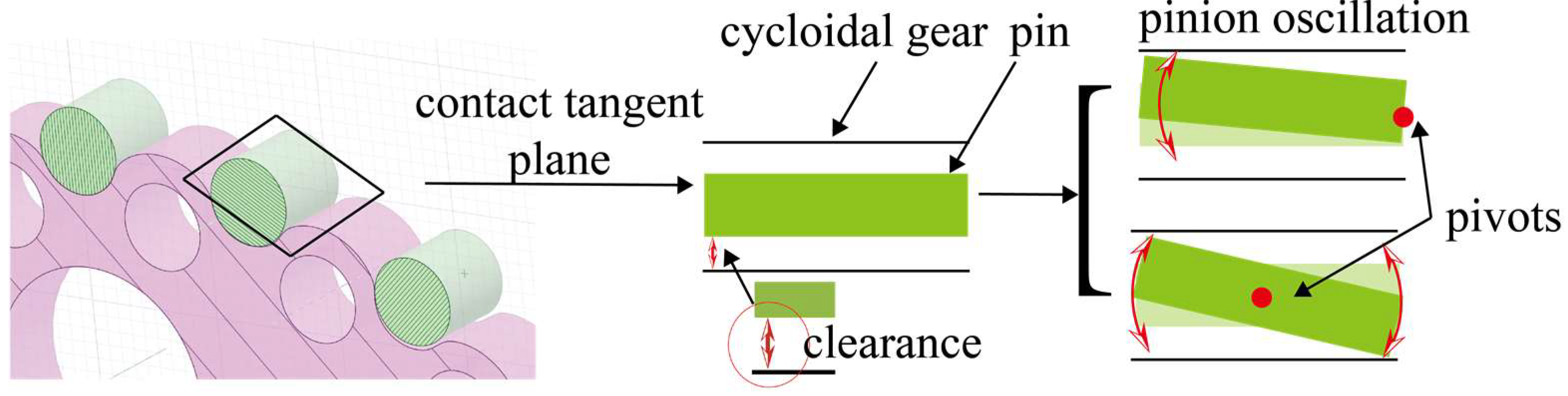
Upon an in-depth examination of the contact surface geometry in conjunction with the actual operational conditions, it becomes evident that the clearance during the meshing process between the pinion teeth and the cycloid gear leads to the misalignment of the axes of the two contacting bodies. This misalignment culminates in an ellipsoidal paraboloid-shaped contact region. Moreover, the oscillation or ‘runout’ of the pinion teeth undeniably has repercussions on the stress distribution across the face of the cycloid gear, as shown in Figure 2.

In scenarios considering pinion oscillation, this analysis operates on the presumption of contact between infinitesimally small convex bodies. The pressure distribution on the contact surface, under these circumstances, still conforms to the Hertzian stress distribution model. Notably, we disregarded any contact effects beyond the direct meshing of the pinion with the cycloid gear. This means that during the ‘runout’ phase of the pinion, there are no other collisions to account for.

To sum up, when the pinion engages with the cycloid gear, the situation can be approximated as the contact problem of two cylindrical bodies with misaligned axes. The deformation at the contact site manifests as an ellipsoidal paraboloid. Hence, when computing the contact forces between the cycloid and the pinion, the impact of a conical contact surface on the force dynamics is incorporated into the analysis.

Assuming that the angle between the axes of two cylinders is $\theta$, where $\theta \in \left(0^{°},{90}^{°}\right]$, it should be noted that when $\theta$ is 0°, the relationship between the contact force and deformation between the cylinders is linear, and a different contact force model is used; hence, this value is not included in the range. In addition, the radii of the two cylinders are R₁ and R₂, respectively. It is possible to calculate the heights of the two surfaces near the contact point, as shown in Equation (9).

$$h=z_1+z_2=\frac{x^2}{2R_1}+\frac{{(x\cos \theta -y\sin \theta )}^2}{2R_2}$$

(9)

where R₁ and R₂ denote the radii of the two cylinders, respectively.

By forming a quadratic form through the surface height h, the principal curvatures can be obtained, and consequently, the results for the equivalent radius are derived. This allows for the substitution of the equivalent rigid sphere and elastic half-space body contact force model (which is identical to the computational model used when the angle between the axes is 90°), as shown in Equation (10).

$$F=\frac{4}{3}{E}^{*}{\tilde{R}}^{1/2}{d}^{3/2},$$

(10)

The aforementioned formulas are based on the assumption of small deformations and that the cylindrical bodies are made of linear elastic materials. Under the conditions of complete contact, these equations are derived from the Hertzian contact theory model. The contact force F can be expressed as Equation (11).

$$F=\frac{4}{3}{E}^{*}{(R_1{R}_2)}^{1/4}{d}^{3/2}{\cos }^{3/2}\left(\frac{\pi -2\theta }{4}\right)$$

(11)

where $E^{*}$ represents the equivalent elastic modulus, assuming that the material of the cycloid wheel and the pin gear is the same, both being GCr15, $E^{*}=\frac{0.5E}{1-{\nu }^2}$. d represents the contact depth. ${\cos }^{3/2}\left(\frac{\pi -2\theta }{4}\right)$ denotes the ratio of the long and short axes of the ellipse in the contact region, and it takes into account the effect of the angle between the two cylindrical axes on the shape of the contact surface.

3. Analysis Method of End Face Stress for Cycloid Gear

Various methodologies are employed for the computation of stress on gear contact surfaces, including Mechanical Analysis, FEA, Empirical Formulation, the equivalent stress method, and Statistical Analysis. The applicability of these approaches hinges on the specific scenarios they address. While Mechanical Analysis and FEA offer nuanced insights into the stress distribution and magnitude on the contact surface, they mandate a comprehensive understanding of the gear’s structure and material properties, accompanied by intricate computational processes. The Empirical Formulation, albeit restricted in its applicability, proffers the advantages of simplicity and expeditious calculations. The equivalent stress method, despite its rapid computational attributes, has a circumscribed domain of applicability, potentially leading to discrepancies in its outputs. The Statistical Analysis approach is adept at mirroring the gear’s lifecycle characteristics, but it is inherently sensitive to the volume and distribution of data samples.

3.1. Conformal Mapping Method for Multiply Connected Domains

The Schwarz–Christoffel (SC) transformation serves as a keystone in the realm of geometry, facilitating the conformal mapping of the upper half of the complex plane into the interior of polygons. Harnessing the potential of the SC transformation paves the way for the geometrical elucidation of complex functions, enabling a probe into their inherent properties and addressing the boundary value challenges that are prevalent in the spheres of physics and engineering [25,26]. A quintessential representation of the SC formula is typically articulated as follows:

$$\omega =f(z)=C{{\displaystyle \int }}^{z_0}{\displaystyle \prod _{k=1}^n{(z-z_k)}^{a_k-1}}dz+C_1,$$

(12)

where the original vertices of the polygon ${\omega }_k$ correspond to the vertices $z_k$ after being mapped onto the circle. At the point ${\omega }_k$, the turning angle of the tangent to the polygon is $\left(1-a_k\right)\pi$. The constants C and C₁ are set based on the physical boundary conditions.

While the Schwarz–Christoffel (SC) mapping adeptly maps bounded polygons to the unit circle, its utility is confined to simply connected polygonal domains. When addressing bounded multiply connected polygonal regions, Mohamed et al. [27,28] have elucidated an approach grounded in the Koebe iterative method combined with boundary integral equations to ascertain mapping functions and their inverses for these multiply connected domains. This methodology furnishes a numerical implementation to compute circular mappings of multiply connected regions, leveraging the Koebe iterative procedure to approximate the mapping relations.

By discretizing the boundary components and deploying computationally economical algorithms, accurate circular mapping outcomes can be efficiently derived. Specifically, by employing the boundary values gleaned from the Koebe iterative method for bounded multiply connected regions, the mapping values for the interior points of the multiply connected domains can be determined using the Cauchy integral formula, as delineated in Equation (13). In a parallel vein, the Cauchy integral formula facilitates the computation of the values for circular inverse mapping, as presented in Equation (14).

$$w=\omega (z)=\frac{1}{2\pi \mathrm{i}}{\displaystyle {\int }_J\frac{\omega (\eta (t))}{\eta (t)-z}}{\eta }^{\prime }(t)\mathrm{d}t,$$

(13)

where $w$ is the value of the mapping function, representing the point on the complex plane after mapping; $z$ is the point on the complex plane waiting to be mapped; $\omega (\eta (t))$ denotes the value of the mapping function $\omega$ on the parameter curve $\eta (t)$; $\eta (t)$ is the parameter curve describing the path in the bounded region $J$; and ${\eta }^{\prime }(t)$ represents the derivative of the parameter curve $\eta (t)$ with respect to t.

$$z={\omega }^{-1}(w)=\frac{1}{2\pi \mathrm{i}}{\displaystyle {\int }_J\frac{{\omega }^{-1}(\xi (t))}{\xi (t)-w}}{\xi }^{\prime }(t)\mathrm{d}t,$$

(14)

where $z$ is the value of the inverse mapping function, indicating the point mapped to the complex plane; $w$ is the point on the complex plane waiting to undergo inverse mapping; ${\omega }^{-1}(\xi (t))$) signifies the value of the inverse mapping function ${\omega }^{-1}$ on the parameter curve $\xi (t)$; $\xi (t)$ is the parameter curve that outlines the trajectory in the bounded region $J$; and ${\xi }^{\prime }(t)$ is the derivative of the parameter curve $\xi (t)$ with respect to a given parameter.

3.2. Geometric Characteristics of Cycloid Gear Profiles with Pores

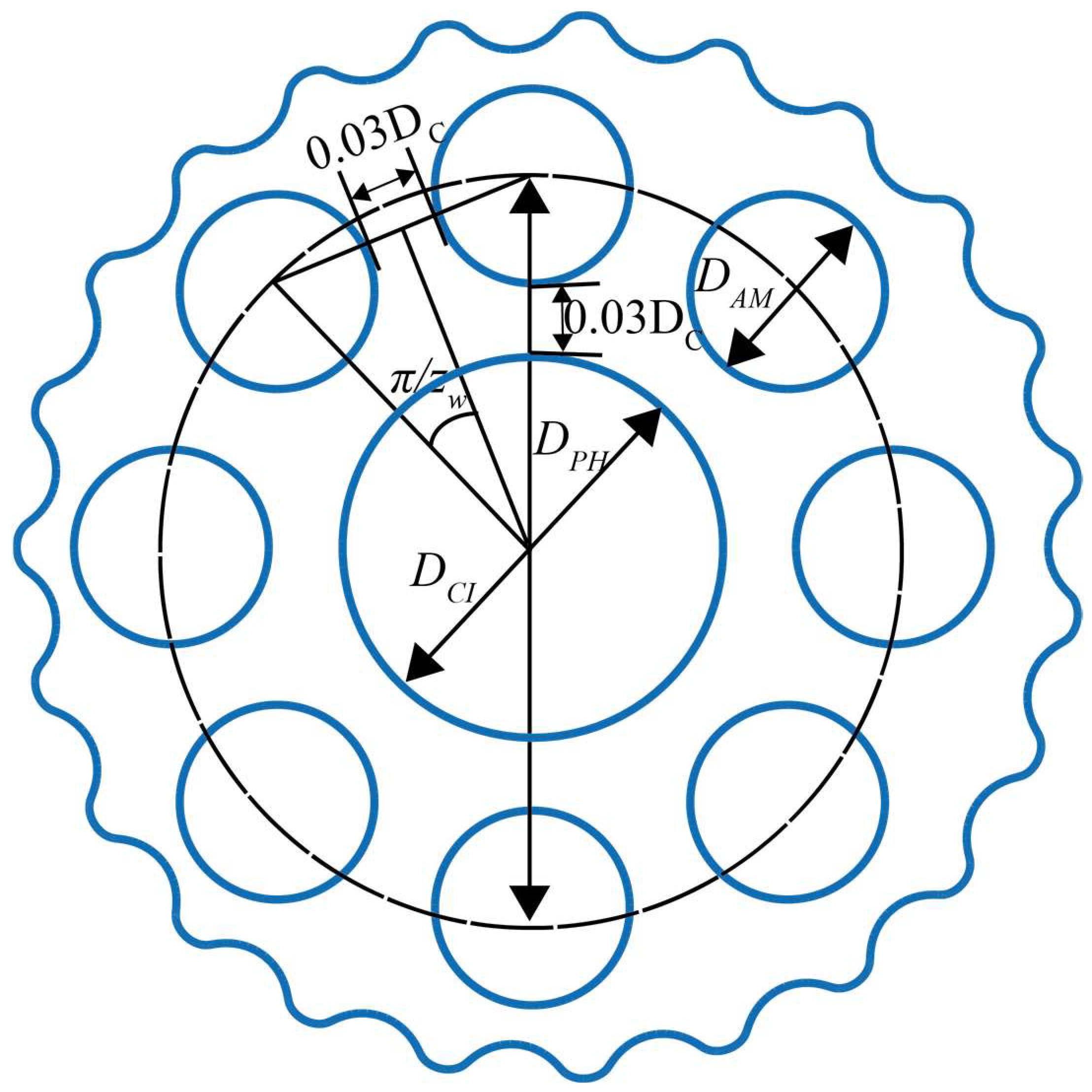
The maximum allowable diameter of the cycloidal gear pinhole is represented by Equation (15). The corresponding pin hole structure arrangement is shown in Figure 3.

$$\left[D_{AM}\right]=\min \left\{\begin{array}{c}{D}_{PH}-D_{CI}-2\times 0.03D_C\\ D_{PH}\sin \frac{\pi }{z_w}-0.03D_C\end{array}\right\},$$

(15)

where $D_C$ signifies the diameter of the cycloidal gear, $D_{PH}$ represents the diameter of the center circle of the cycloidal gear pinhole; and $D_{CI}$ denotes the diameter of the central hole of the cycloidal gear, and in this case, the value of $D_{CI}$ is set to 0.4$D_C$. It can also be determined based on the actual outer diameter of the installed bearing. The variable $0.03D_C$ indicates the empirical minimum wall thickness values for the pin holes.

3.3. SACGES-CMMD Method

By utilizing the dual quaternion cycloid gear tooth profile model delineated by Jiang [29], a collection of vertex coordinates was garnered. With the aid of the Plgcirmap toolbox, the bounded connected polygonal domain was adeptly transformed into a bounded connected unit circle domain. Subsequent to this transformation, boundary vertices were systematically numbered.

During the meshing phase, the areas of the cycloid gear teeth subject to force warranted a localized refinement. Consequently, a mesh gradient of 1.5 was set, and the GeometricOrder was designated as ‘quadratic’. For the boundary conditions, the nodes associated with the central hole were anchored with fixed constraints. Following these configurations, the stress analysis results of the unit circle were then deduced. Ultimately, the coordinates endowed with stress details were inversely mapped from the unit circle back to the polygonal domain. The procedural workflow of the stress analysis method of the cycloid gear end surface based on conformal mapping in multi-connected domains (SACGES-CMMD) is vividly depicted in Figure 4.

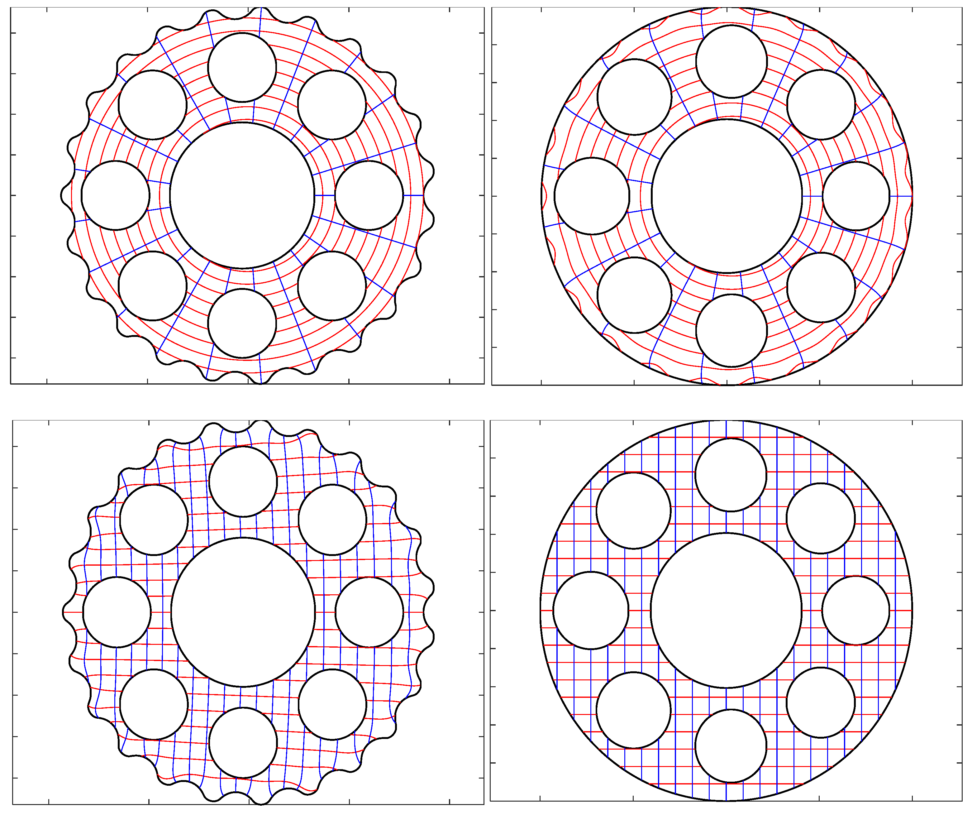
In the framework of this analysis, a bounded polygonal connected domain boasting a connectivity value of 10 was explored. To capture the conformal mapping of this domain, the ‘plgcirmap’ function in MATLAB 2020b was employed, leveraging the vertices of the polygon and selected points within the domain. During the mapping computation, normalization was invoked. The resultant conformal mapping, f, and its inverse, f⁻¹, were pictorially represented using the ‘plotmap’ function, as evinced in Figure 5.

In this investigation, an intricate mapping procedure was carried out, converting the node information from a bounded multiply connected region, specifically the epitrochoid area, to a unit circle. Building on this, the MATLAB PDE toolbox was employed to execute a stress analysis on the unit circle, delineating the process from stages (c) to (d), as shown in Figure 4. The subsequent inverse mapping process from the unit circle back to the polygonal region, embedding the stress information, necessitates the computation of the Jacobian matrix, executed as follows:

(1)

Initialization: For a designated polygonal region coupled with its associated stress tensor distribution, the position of each node (polygon vertex) and its corresponding first-order derivative are computed. Special attention is devoted to instances where the first-order derivative is zero, circumventing potential numerical complications in ensuing computations.

(2)

Computation of Jacobian Matrix for Inverse Mapping: Upon obtaining the node data and first-order derivatives, the Jacobian matrix for inverse mapping at each node is ascertained. The Jacobian is informed by the complex derivative of the inverse mapping function. By inputting complex variable details representing the unit circle node into the inverse mapping function, the correlated polygon node data are derived, and the differential from this reverse mapping (from the unit circle to the polygon) is secured. When constructing the Jacobian matrix, the derivative of the complex variable, normalized by its magnitude, is bifurcated into real and imaginary parts, serving as matrix elements. This protocol adheres to the Cauchy–Riemann equations characterizing complex functions. The result functions as a local Jacobian matrix for rotation and scaling at the node.

(3)

Mapping of Stress Tensor: During inverse mapping, the stress tensor on the unit circle is projected to nodes within the polygonal region. The need for scaling stems from the disparities in the dimensional magnitudes across the polygon. To accurately capture the stress levels, especially given the diverse stress distribution in various regions, a uniform global scaling factor is introduced based on the specific contour dimensions of the shape. This ensures a more authentic representation of the stress distribution throughout the domain. Additionally, each node might undergo local rotation and scaling, as described in step 2. These transformations are assessed in relation to the local node coordinate system, necessitating individual node calculations. When integrating these local adjustments with the global stress scaling influenced by dimensional magnitudes, a holistic and precise depiction of the stress distribution within the polygon emerges. It is crucial to balance the considerations of this uniform global scaling factor with the local rotational and scaling intricacies during stress tensor mapping within the polygonal domain. This study not only underscores this integration but also dives deep into the implications of the global scaling factor, laying the groundwork for subsequent inquiries in this domain.

(4)

Storing Mapping Outcomes: The stress tensor derived from mapping is archived within a novel matrix representing the stress distribution within the unit circle, culminating the tensor mapping from the polygonal to the unit circle domain.

3.4. Global Stress Scaling Factor

Considering the size discrepancy at the millimeter scale between the shape and the unit circle, a global stress scaling factor is employed in this paper for normalization purposes. As depicted in Figure 6, by holding the distance between the fixed point and the point of applied force constant, the alterations in the shape of the force-applied region have negligible impacts on the resultant maximum equivalent stress. When ensuring consistency in the mesh count, as per the representation in Figure 7, an inverse relationship between the maximum equivalent stress value and side length is evident. Their product, however, demonstrates minimal fluctuations. From the above observations, during the mapping process, it is discerned that the factors affecting the peak stress predominantly hinge on variations in the geometric dimensions, with shape deviations playing marginal roles.

In light of these findings, this paper introduces a methodology for computing the average radius of a polygon centered on its geometric centroid, which essentially serves to determine the scaling factor. The initial step merges the horizontal and vertical coordinates of each vertex of the polygon into a singular matrix. Subsequently, the geometric centroid of the polygon is ascertained. The ensuing step involves calculating the Euclidean distances from each vertex to the geometric centroid. The average of these distances renders the polygon’s average radius. The core intent behind this strategy is to harness the average radius as a pivotal reference value during geometric scaling transformations.

For a more formal representation, consider P as a two-dimensional polygon comprising n points, with the coordinates for each point delineated as (x_i, y_i), where i = 1, 2, …, n. Consequently, the average radius r_avg of the polygon P can be articulated as per Equation (16).

$$r_{\mathrm{avg}}=\frac{1}{n}{\displaystyle \sum _{i=1}^n\sqrt{{\left(x_i-\frac{1}{n}{\displaystyle \sum _{j=1}^n{x}_j}\right)}^2+{\left(y_i-\frac{1}{n}{\displaystyle \sum _{k=1}^n{y}_k}\right)}^2}}.$$

(16)

Given the context established in this study, the stress transformation process is delineated from unit circle inversion mapping to the polygon. Hence, the scaling factor is determined as 1/r_avg. Assuming that, during the variations in the geometric shape dimensions, the product of the stress and the scaling factor remains constant, this approach facilitates the determination of the stress across the cycloid gear cross section.

4. Bayesian-Enhanced Least Squares Genetic Algorithm Optimization Method

When integrating the research contents of Section 2 and Section 3, there is a need for an optimization algorithm to address the stress distribution optimization problem, considering the errors and random fluctuations in the contact force. In this study, we introduce the BLSGAOM, an innovative approach that seamlessly integrates Genetic Algorithms (GAs) with Least Squares Boosting Models, as shown in Algorithm 1. Initially, GA parameters are established within specified bounds, after which an iterative optimization, steered by BLSGAOM’s fitness function, adapts and fine-tunes these parameters. The specific settings for the input parameters are as follows: in the authors’ previous study [29], three error values were identified as the input parameters, with their respective numeric bounds defined as [0 mm, 0.1 mm], [0 mm, 0.04 mm], and an unspecified range denoted by [$0^{\prime },\hspace{0.17em}\hspace{0.17em}10^{\prime }$]. The three represent the bending deformation of the input crankshaft, the amount of pinion runout, and the hysteresis angle, respectively.

Algorithm 1 Bayesian-enhanced least squares genetic algorithm optimization model

Step Procedure

1 Set Genetic Algorithm Parameters: nvars← 3

lb← [0, 0, 0]

ub← [0.1, 0.04, 10/60]

2 Initialize Genetic Algorithm Options:

options ← SET Display to ’iter’, Migration Interval to 20, Migration Fraction to 0.3

bestFvals←$\Phi$

3 (x, fval) ← GA using fitnessFunction, lb, ub, and options

4 Display optimal solution and fitness: x, fval

5 Plot evolution of Best Fitness Value:

PLOT bestFvals vs. Generation

6 Function fitnessFunction(x):

ypred ← LSBM_predict_result(x1, x2, x3)

return ypred

7 Function outfun(options, state, flag): UPDATE bestFvals with min(state.Score)

DISPLAY state’s details

return options, state, optchanged

8 Function LSBM_predict_result(x1, x2, x3): LOAD pretrained model

X ← [x1, x2, x3]

result ← PREDICT with model and X

return result

9 LOAD Dataset

Extract input X and target y Split Dataset using cvpartition

10 Hyperparameter Tuning: Set optimization options results ← BAYESOPT

11 Train bestModel using FIT with optimal parameters

12 Predict: ypred ← PREDICT using bestModel and X

13 Compute metrics: MSE, RMSE, MAE, R2

14 Save trained model

15 Plot Actual vs. Predicted

A salient feature of our BLSGAOM is its adept utilization of surrogate models during the Bayesian optimization phase. These surrogate models have become indispensable tools in engineering design, offering substantial advantages, especially when faced with computationally challenging tasks. The incorporation of surrogate models offers a dual benefit: they significantly reduce the computational overhead by efficiently approximating complex problem behaviors and provide flexibility, enabling the seamless application of classical optimization algorithms. This malleability helps to sidestep potential pitfalls such as local optima and high computational costs, which are often inherent to the original problem.

Moreover, surrogate models enhance the interpretability of the foundational problem, making them invaluable in contexts where understanding the nuances of the problem is crucial. In scenarios characterized by expansive or intricate design spaces, these models proficiently navigate, identifying solutions that best align with specific criteria. Their inherent adaptability means they can easily assimilate new data, ensuring continuous refinement in their precision and efficiency.

By leveraging the strengths of these surrogate models, BLSGAOM provides a judicious approximation to the true objective function. This methodological approach ensures thorough exploration and exploitation of the hyperparameter space without resorting to excessive evaluations of the primary objective. The culmination of this process is a refined model armed with optimal settings. To validate the robustness of our model, the predictions are critically assessed using a suite of error metrics, providing a holistic view of its performance and reliability. The optimized model is shown in Equation (17).

$$\begin{array}{cc}\mathrm{minimize}& f(b,f,d)=\max (\sigma (b,f,d))+\mathrm{var}\left({\sigma }_{\mathrm{dist}}(b,f,d)\right)\\ \mathrm{s}.\mathrm{t}.& 0\le {\Delta }_b\le 0.1\\ & 0\le {\Delta }_f\le 0.04\\ & 0^{\prime }\le {\Delta }_d\le {10}^{\prime }\end{array}$$

(17)

where $f(b,f,d)$ represents the objective function of optimization; $\sigma (b,f,d)$ represents the maximum stress induced by the error terms; and ${\sigma }_{\mathrm{dist}}(b,f,d)$ represents the stress distribution caused by the error terms.

5. Results and Discussion

5.1. Results of Clearance Effect on Contact Force Fluctuation

For relatively minute angular deviations, as illustrated in Figure 2, the range of angular values can be approximated to the ratio of the clearance to pinion length and half of the clearance over the pinion length. Specifically, when the clearances are set at 10 μm, 20 μm, and 30 μm, respectively, they correspond to the angular variations of [0.001 rad, 0.002 rad], [0.002 rad, 0.004 rad], and [0.003 rad, 0.006 rad]. Within these bounds, the relationship between the contact force and contact depth is depicted in Figure 8. Post the establishment of a slight angular discrepancy due to the clearance, there is an overall reduction in the contact force. Additionally, as the clearance marginally increases within a certain range, there is a subtle rise in the contact force.

5.2. Accuracy Results for Conformal Mapping

In the present study, a meticulous computation and an analysis were conducted on the errors at a series of test points for complex functions. Initially, a set of test points were uniformly sampled on the unit disk, and through the inverse mapping of the complex functions, these points were correspondingly mapped to a collection on the complex plane, as illustrated in Figure 9a. Subsequently, the discrepancies between each test point and its associated point post inverse mapping were evaluated, with the maximum norm employed as the metric for error quantification.

According to the computed outcomes, a parabolic trend in the distribution of errors between the test points and their inversely mapped counterparts was discerned, as depicted in Figure 9b. Within this error distribution, the maximum error norm was found to be 2.7280 × 10⁻¹¹, signifying that the inverse mapping method exhibited exemplary performance in the majority of instances. Such a method could accurately preserve the relationship between the test points and the original points, underscoring its robustness and precision.

5.3. SACGES-CMMD vs. FEM Comparison Results

The SACGES-CMMD, in contrast to the FEM, brings forward a set of unique advantages. Central to these is the conformal mapping technique, which preserves angular relationships within multi-connected domains. This ensures that the stress patterns on a mapped unit circle accurately reflect those of the original polygonal domain. This geometric preservation, coupled with a scaling factor, streamlines stress computations. Additionally, this method boasts greater numerical stability, minimizing the potential instabilities and singularities that are often associated with direct FEM calculations on polygons. Moreover, applying the FEM on the unit circle guarantees a uniformly distributed grid, benefiting from the circular domain’s inherent regularity and thereby heightening the computational precision. Furthermore, the straightforward circular geometry of the stress distribution facilitates an enhanced visualization and comparability of the results. Collectively, the use of conformal mapping for stress distribution in multi-connected domains enhances geometric integrity, numerical robustness, grid uniformity, and the clarity of the visualization and analysis.

From a comparative analysis of the results obtained using the FEM and SACGES-CMMD, as depicted in Figure 10 and summarized in

Table 1. Comparison of FEM and SACGES-CMMD results.

	Scaling Factor	Maximum Mesh Size (mm)	Minimum Mesh Size (mm)	Mesh Gradient	Number of Nodes	Percentage Reduction (%)	Maximum Shear Stress (MPa)	Stress Distribution STD	Computation Time (s)	Percentage Reduction (%)
FEM	0.0892	0.892	0.0892	1.5	98,202	7.34	11.01	0.1028	18.95	−0.11
SACGES-CMMD		10	1		90,992		10.07	0.1275	18.97
FEM	0.0898	1.3470	0.0988		55,896	12.31	10.65	0.1296	17.21	−0.29
SACGES-CMMD		15	1.1		49,020		10.09	0.1749	17.26
FEM	0.0900	1.8	0.0990		46,758	15.63	10.72	0.1421	17.03	4.75
SACGES-CMMD		20	1.1		39,451		10.12	0.1931	16.22
FEM	0.0904	2.712	0.0994		38,654	19.34	10.68	0.1555	16.56	3.45
SACGES-CMMD		30	1.1		31,178		9.47	0.2135	15.99

, four key observations can be drawn:

(1)

Grid Scale and Gradient Consistency: Under equivalent computational conditions, both methodologies exhibited grid sizes and gradients of comparable scales.

(2)

Optimized Grid Utilization with SACGES-CMMD: Notably, the SACGES-CMMD approach utilized marginally fewer grid nodes than its FEM counterpart. The smallest reduction ratio in the number of nodes was 7.34%. As the mesh size increased, the reduction ratio in the nodes gradually increased as well, reaching up to 19.34% in the end. This suggests that the conformal mapping process underpinning SACGES-CMMD permits the elimination of superfluous grid elements, thereby optimizing computational efficiency within a compact grid layout.

(3)

Comparative Stress Metrics: The comparison highlighted a close correspondence between the maximal shear stress and the stress distribution’s STD for both methods, with no significant disparities discernible.

(4)

Computational Efficiency: While the computation durations of both techniques were roughly commensurate, a downward trend in the grid element count conferred the SACGES-CMMD with a slight edge in the computational expediency. In the comparison of the computational efficiency, when the mesh was dense, both exhibited similar efficiencies with variations of 0.11% and 0.29%, respectively. As the mesh size increased, the computational efficiency of SACGES-CMMD showed a significant improvement, reaching a peak of 4.75%.

When synthesizing these insights, it becomes evident that while SACGES-CMMD parallels the FEM in terms of computational precision and reliability, it proffers certain advantages. Namely, these comprise a leaner grid element composition and a modest reduction in the computation time. Consequently, SACGES-CMMD emerges as a viable strategy for stress distribution evaluations in multi-connected domains, holding potential for elucidating the characteristic stress distribution patterns within such domains. This stress analysis method provides a thought process for model equivalence transformation to solve the issue of computational infeasibility of the solid model before and after the cycloidal wheel modification across large-scale grid divisions. This is due to the fact that the amount of modification is at the micron level, while the tooth profile shape is at the millimeter level. It offers a solution for large-scale grid divisions in computational models.

5.4. Optimization Results of Stress Distribution Based on BLSGAOM

Drawing upon the parameter design presented in

Table 2. Design parameters of the cycloid-pin system for SACGES-CMMD.

Parameters	Values	Parameters	Values
Loading torque, T (Nm)	600	Number of teeth of cycloid gears, za	23
Density, ρ (Kg/m3)	7830	Pinion number, zb	24
Poisson’s ratio, $\nu$	0.3	Pitch radius of pin teeth, rb (mm)	72
Pin tooth center circle radius, Rb (mm)	100	Pitch radius of the cycloid gear, ra (mm)	69
Eccentricity, e (mm)	3	Pin tooth radius, rp (mm)	10
Elastic modulus, E (GPa)	208

, the contact force dynamics of the gear tooth profile are dissected. This analytical framework then sets the stage for the integration of conformal mapping techniques specific to multi-connected domains. The intricate cycloidal gear tooth profile is seamlessly mapped onto a unit circle through this approach.

The magic of this conformal mapping lies in its transformative capability; it simplifies the complex contour of the gear tooth to the elementary geometry of a unit circle. As alluded to in Section 3.3, utilizing the approximate relationships of the scaling factors enables the stress distribution results, which were originally derived from the FEM on the unit circle, to be inversely mapped onto the cycloidal gear tooth profile. This technique substantially curtails the computational overhead that is typically associated with stress distribution calculations, offering both efficiency and precision.

For this study, the Least Squares Boosting (LSBoost) method was enlisted to train the machine learning models. This endeavor commenced with the segregation of the dataset; of the 1000 data instances, 80% fueled the training phase, while the remaining 20% were earmarked for testing. Two pivotal hyperparameters—the learning rate and the number of learning epochs—were subjected to rigorous optimization. Specifically, the learning rate oscillated between 0.01 and 0.2, whereas the epochs ranged from 50 to 200. The Bayesian optimization, as depicted in Figure 11, underpinned the hyperparameter tuning phase, selecting the optimum values based on the anticipated improvements. The k-fold cross-validation technique was employed during model training to ensure both a robust assessment of the performance and a bulwark against overfitting. Upon finalizing the hyperparameters, the model was trained using the dataset and subsequently engaged in predictions.

To rigorously evaluate the predictive capacity of the model, we employed a comprehensive set of critical performance metrics. The Mean Square Error (MSE), a key indicator of the predictive accuracy, denoted an average squared difference of 9.6527 × 10⁻⁷ between the predicted and observed values, highlighting the model’s precision. This precision was further reinforced by the Root Mean Square Error (RMSE), valued at 9.8248 × 10⁻⁴, and the Mean Absolute Error (MAE), which reflected an average deviation of 2.7699 × 10⁻⁴. Additionally, the model’s explicative prowess was exemplified by an R-squared value of 0.9998, indicating that it could account for nearly all the variability in the data, as graphically illustrated in Figure 12. In pursuit of sustained research continuity and replicability, the optimally trained model was archived, priming it for prognosticating fresh datasets. This strategic archiving not only ensures seamless future applicability but also fosters the study’s replicability in analogous scenarios.

In the present investigation, the GA was harnessed for model parameter optimization. Drawing inspiration from the principles of natural selection and genetic mechanics prevalent in biological evolution, the GA emerges as a heuristic global optimization approach renowned for its exemplary global search capabilities.

The predictive model derived earlier was amalgamated with the three error terms, serving as the basis to forecast outcomes based on the input parameters. Thus, the predictions that were generated constituted the fitness function for the GA, with the overarching objective being the identification of the input parameters that optimize (minimize in this context) the aggregate of the maximum stress and the stress distribution STD.

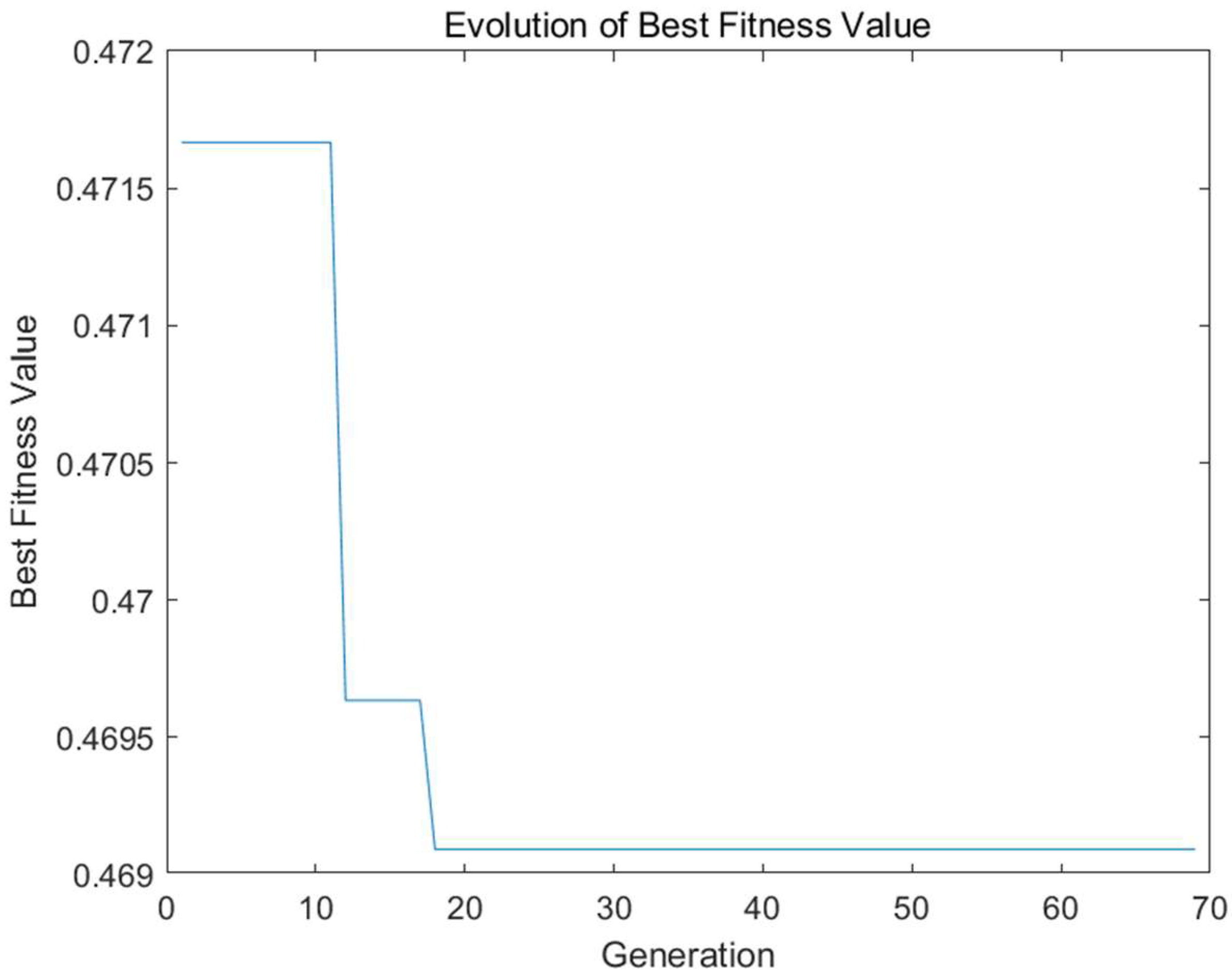
In this study, the configuration of the GA parameters was elucidated as follows: The solution vector length was set at three, directly corresponding to the three error terms. The defined search space bounds ranged from a lower boundary of [0 mm, 0 mm, 0°] to an upper boundary of [0.1 mm, 0.04 mm, 10/60°]. The output functions were integrated to record the optimal fitness values upon the conclusion of every generation. To bolster population diversity and sidestep the potential challenges of the local optima, migrations were programmed at intervals of every 20 generations, with each migration facilitating a randomized transfer of 30% of the population. When the GA was executed, the resulting optimal solution was pinpointed at [0.0641 mm, 0.0058 mm, 0.0584°]. This solution corresponded to a peak fitness (predictive error) value of 0.4691. A graphical representation depicting the progression of the optimal fitness value across generational transitions can be found in Figure 13.

5.5. Optimization Results of Stress Distribution Considering Contact Force Fluctuations

In the assembly, deviations manifesting as gear tooth jitters emerge due to the assembly clearances, subsequently leading to alterations in the contact forces. As stipulated by Equation (11), a rectification term, ${\cos }^{3/2}\left(\frac{\pi -2\theta }{4}\right)$, is incorporated during the computation of the contact forces. As with the parameter configurations delineated in Section 5.4, the optimization trajectory is vividly portrayed in Figure 14.

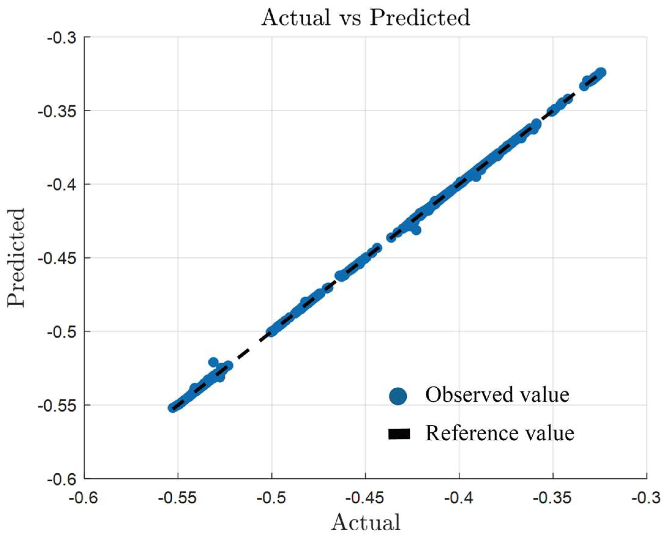
Ultimately, the performance metrics of the predictive model were elucidated as MSE = 6.8474 × 10⁻⁸, RMSE = 2.6168 × 10⁻⁴, and MAE = 4.6979 × 10⁻⁵, and the coefficient of determination, R², stood at 1. Collectively, these indices underscore the model’s robust explanatory power concerning the data, as graphically elucidated in Figure 15.

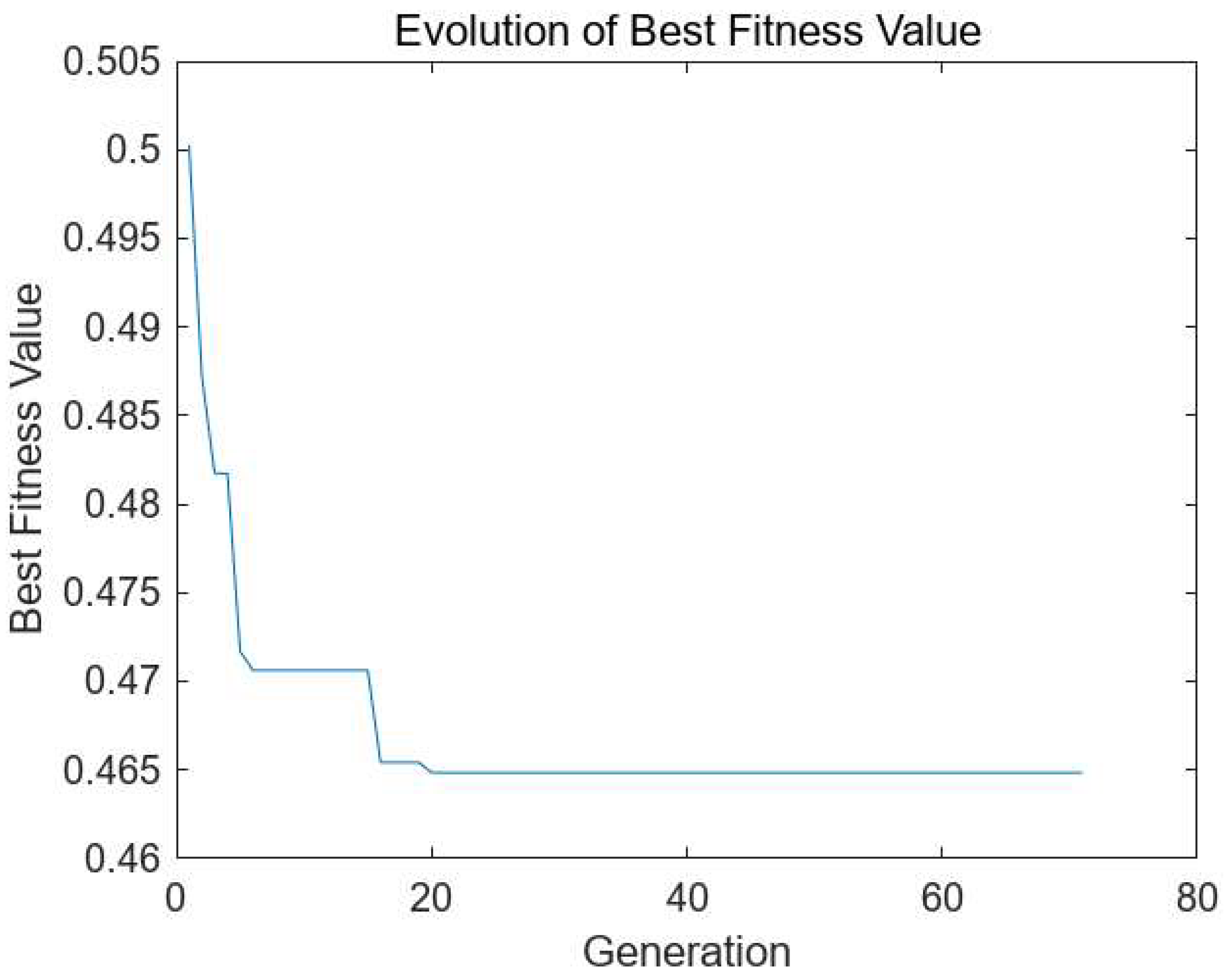
Upon the execution of the genetic algorithm, the optimal solution procured was [0.0645 mm, 0.0083 mm, 0.0819°]. This corresponds to an optimal fitness value (i.e., predictive error) of 0.4648. The trend of this optimal fitness value in relation to the number of generations can be visually represented in Figure 16.

In the comprehensive analysis on the stress distribution in the cycloid-pin gear systems, two distinct methodologies were adopted: one that factored in the nuances of the contact force fluctuations and another that disregarded these fluctuations. Before incorporating the effect of the contact force fluctuations, the Bayesian-enhanced least squares boosted surrogate model exhibited an R-squared value of 0.9998, an MSE of 9.6527 × 10⁻⁷, an RMSE of 9.8248 × 10⁻⁴, and an MAE of 2.7699 × 10⁻⁴. This model predicted an optimal error configuration of [0.0641 mm, 0.0058 mm, 0.0584°] with a predictive error (or fitness value) of 0.4691.

Upon the consideration of contact force fluctuations, brought about by gear tooth jitters due to assembly clearances, the model’s performance metrics exhibited an even higher fidelity. The R-squared value reached perfection, standing at 1, while the MSE, RMSE, and MAE values were reduced to 6.8474 × 10⁻⁸, 2.6168 × 10⁻⁴, and 4.6979 × 10⁻⁵, respectively. The optimal error values in this scenario were [0.0645 mm, 0.0083 mm, 0.0819°], corresponding to a slightly improved predictive error of 0.4648.

The observed improvements in the model’s performance metrics when accounting for the contact force fluctuations underpin the significance of considering such dynamic effects in the optimization process. By ensuring a holistic view of the system behavior, this study provides a pivotal foundation for more accurate predictive modeling and optimization in gear systems.

6. Conclusions

In this exploration to optimize the end face stress distribution of cycloidal gears, a parabolic contact surface between two cylindrical bodies was deduced, leading to the establishment of a model relating the contact force to the axis angle (between two axes) under varying clearances, and obtaining the corresponding impact factor. Concurrently, the adoption of the conformal mapping technique facilitated the geometric and stress transitions between the polygons and a unit circle. By harnessing the intricate multi-connected domain tooth profile of the cycloidal wheel, the approach synergized conformal mapping with a global stress scaling factor, promoting a reverse mapping from the unit circle to the polygons, and thereby determining the end face stress of the cycloidal wheel. The SACGES-CMMD methodology, compared to the FEM, showcased fewer grid divisions with a reduction ratio reaching up to 19.34%, improved computational efficiency peaking at 4.75%, and retained precision. To conclude, the employment of the Bayesian-enhanced least squares surrogate model combined with the genetic algorithm sought to minimize the sum of the maximum stress and the stress distribution STD as the optimization objectives. The objective of achieving a uniform stress distribution was attained by optimizing the operating error parameters and adjusting the design of the cycloidal gear profile. This endeavor yielded optimal solutions manifested as [0.0641 mm, 0.0058 mm, 0.0584°] and [0.0645 mm, 0.0083 mm, 0.0819°], underscoring the promise and relevance of the approach and illuminating avenues for future advancements and potential applications in the realm of gear end face stress analysis.