SliceSamp: A Promising Downsampling Alternative for Retaining Information in a Neural Network

Featured Application

Plug-and-play downsampling module SliceSamp provides support for deploying AI models on edge computing devices, powering neural networks with lighter weights, lower computational costs, and higher performance.

Abstract

Downsampling, which aims to improve computational efficiency by reducing the spatial resolution of feature maps, is a critical operation in neural networks. Many downsampling methods have been proposed to address the challenge of retaining feature map information. However, some detailed information is still lost, even though these methods can extract features with stronger semantics. In this paper, we propose a novel downsampling method which combines feature slicing and depthwise separable convolution for information-retaining downsampling. It slices the input feature map into multiple non-overlapping sub-feature maps by using indexes with a stride of two in the spatial dimension and applies depthwise separable convolution on each slice to extract feature information. To demonstrate the effectiveness of SliceSamp, we compare it with classical downsampling methods on image classification, object detection, and semantic segmentation tasks using several benchmark datasets, including ImageNet-1K, COCO, VOC, and ADE20K. Extensive experiments demonstrate that SliceSamp outperforms classical downsampling methods with consistent improvements in various computer vision tasks. The proposed SliceSamp shows advanced model performance with lower computational costs and memory requirements. By replacing the downsampling layers in different network architectures (including ResNet (Residual Network), YOLOv5, and Swin Transformer), SliceSamp brings different degrees of performance gains (+0.54~3.64%) compared to these baseline models. Additionally, SliceUpsamp enables high-resolution feature reconstruction and alignment during upsampling. SliceSamp and SliceUpsamp can be plug-and-play-integrated into existing neural network architectures. As a promising downsampling alternative to traditional methods, SliceSamp can also provide a reference for designing lightweight and high-performance model architectures in the future.

1. Introduction

In recent years, deep learning [1] has achieved remarkable success in various computer vision (CV) tasks, such as image classification [2], object detection [3,4], and semantic segmentation [5]. However, deep learning (DL) models often suffer from heavy computational burdens due to large numbers of parameters and high-dimensional input data, limiting their practical applications [6]. In particular, the proliferation of smart devices and IoT (Internet of Things) sensors has given rise to a pressing need for edge computing [7] as edge computing enables computation near data sources or things. To deploy DL models on resource-limited edge devices, reducing model complexity has become a priority [8,9]. Various techniques have been proposed for reducing the complexity of DL models, among which downsampling plays a crucial role [10]. However, most existing downsampling methods tend to lose some detailed information [11]. Thus, it remains a challenging problem to design a lightweight and efficient downsampling component which can retain more semantic and detailed information with lower algorithmic complexity. In this article, we address this issue by proposing a novel, high-performance slicing downsampling component.

In many computer vision tasks, neural network downsampling is a crucial technique that is used to reduce the spatial resolution of the feature map [11,12]. It can effectively reduce the computational and memory requirements of the network and expand the receptive field while retaining important information for subsequent processing [13]. It reduces the spatial resolution by proportionally scaling down the width and height of feature maps, which can be achieved by selecting a subset of features or by aggregating the features in local regions. Downsampling can help to regularize the network and prevent overfitting by reducing the number of parameters and introducing some degree of spatial invariance [14]. It can improve the efficiency of the neural network in processing large-scale complex data, such as remote sensing images and videos, and enable the DL models to operate on resource-limited devices [15]. Pooling or subsampling of feature maps, such as Max Pooling or Strided Convolution, is a common downsampling operation in the neural network [16]. However, most of the methods condense regional features to a single output, which suffers from several challenges, such as information loss and spatial bias [11]. For instance, Max Pooling only retains the most distinguishable features [17], and subsampling picks a portion of features randomly or according to rules [18,19], while the slicing adopted in this work utilizes the full information in the input feature map, as shown in Figure 1. Therefore, the research on neural network downsampling is still an active area where there is space for optimization, and more efficient methods need be developed for better retaining feature information.

Upsampling also plays an important role in neural networks. It is often used for image super-resolution [20], segmentation [21], and generation [22] tasks via the reconstruction of high-resolution feature maps during the decoding stage in the neural network [23]. The main upsampling methods include interpolation-based upsampling such as the Nearest Neighbor, Bilinear, and Bicubic Interpolation methods [24] and the Transposed Convolution [25] and Sub-Pixel Convolutional [26] methods. The simplest and fastest algorithm is Nearest Neighbor sampling in which each pixel is copied in four copies to a 2 × 2 neighborhood; however, jagged edges are often introduced [27]. The Bilinear and Bicubic Interpolation methods calculate new pixel values via the weighted averaging of the nearest pixels in the original image, providing smoother results than Nearest Neighbor Upsampling yet still introducing some blurring [28]. Transposed Convolution, also known as deconvolution or fractionally strided convolution, is the reverse operation of convolution. It produces high-quality results with an expensive computational burden [29]. Sub-Pixel Convolutional Upsampling rearranges the feature maps via a periodic shuffling operator to increase the spatial resolution [26]. It is fast and computationally efficient; however, it may lead to some artifacts. Many existing downsampling techniques are often combined with the above upsampling methods as it is difficult to implement an inverse transform for generating low-dimensional spatial features [11]. However, our proposed feature-slicing method can reconstruct high-resolution feature maps by reorganizing a feature map to enable the upsampling operation.

In this paper, we present a comprehensive review of state-of-the-art downsampling methods in neural networks, focusing on their advantages and disadvantages, theoretical properties, and practical applications. To overcome the limitations faced by existing downsampling methods, we intend to develop a simple downsampling method that achieves efficient feature extraction and captures channel importance with low computational complexity without discarding the semantic and detailed information of the feature maps. The main contributions of this paper are described briefly below.

(1)

A novel downsampling method based on feature slicing and depthwise separable convolution, SliceSamp, is proposed which is designed to retain all feature information while optimizing computational efficiency.

(2)

An upsampling component, SliceUpsamp, is constructed by reconstructing the feature maps from the channel dimension to the spatial dimension, enabling the inverse operation of downsampling.

(3)

An ablation study is introduced to evaluate the effectiveness of the key design elements. The proposed method can achieve a better balance between algorithmic complexity and model performance.

(4)

Extensive experiments are conducted via various computer vision tasks, including image classification, object detection, and semantic segmentation, based on several benchmark datasets. Our method exhibits significant advantages over classical downsampling methods by replacing the original downsampling layers in different network architectures.

The rest of this paper is organized as follows. Existing work relating to downsampling methods and depthwise separable convolution is reviewed in Section 2. The algorithmic concept and network architecture of the proposed method are described in Section 3. The dataset, implementation details, the results of experiments on a variety of computer vision tasks, and ablation studies are reported in Section 4. Study limitations and future work are discussed in Section 5. The conclusions of this work are summarized in Section 6.

2. Related Works

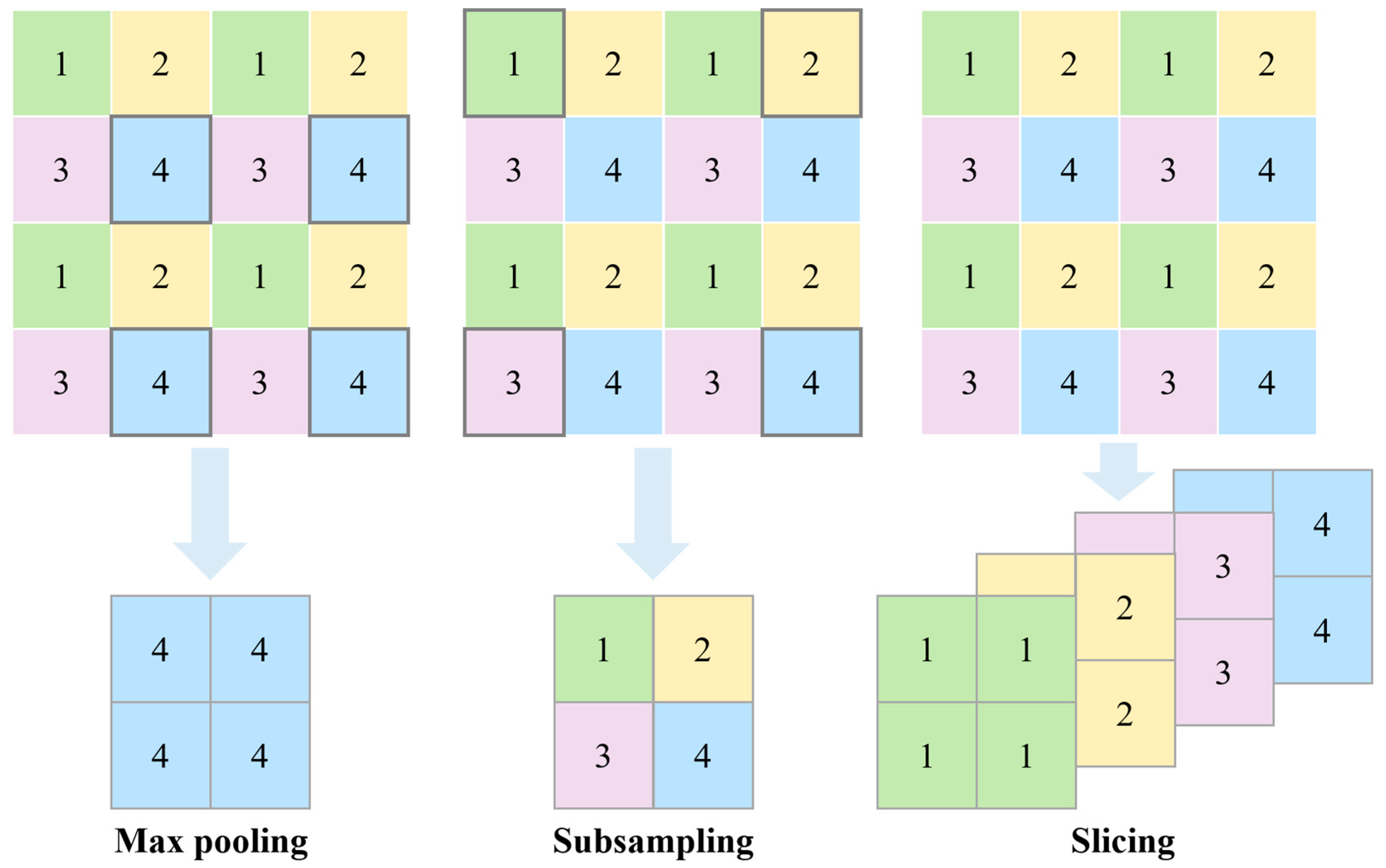
2.1. Downsampling in Neural Networks

To reduce model complexity, researchers have developed various downsampling methods that are tailored to specific tasks and architectures, including pooling-based [17,19], subsampling-based [16,30], patch-based [31,32], and learnable pooling [19,33] methods. In the early stages of neural network development, Maximum Pooling or Average Pooling were commonly adopted to achieve downsampling by taking the maximum or average value within a local window. These methods are fast and memory-efficient, yet t room for improvement remains in terms of information retention [11]. Some methods that combine Max and Average Pooling, such as Mixed Pooling [34], exhibit better performance compared to a single method. Unlike Maximum Pooling, Average Pooling, and their variants, SoftPool exponentially weights the activations using Softmax (normalized exponential function) kernels to retain feature information [12]. Wu et al. [35] proposed pyramid pooling for the transformer architecture; pyramid pooling which applies different scales of average pooling layers to generate pyramid feature maps, thus capturing powerful contextual features. There are also pooling methods that are designed to enhance the generalization of a model. For example, Fractional Pooling [36], S3Pool [13], and Stochastic Pooling [30] can prevent overfitting by taking random samples in the pooling region. However, most pooling-based methods are hand-crafted nonlinear mappings which usually employ fixed, unlearnable prior knowledge [37].

Nonlinear mapping can also be generated by overlaying complex convolutional layers and activation functions in a deep neural network (DNN) [16]. When the network is shallow, pooling has some advantages. When the network goes deeper, multi-layer stacked convolution can learn better nonlinearity than pooling. It can also achieve better results [38]. Therefore, Strided Convolution, which reduces spatial dimensionality by adjusting the stride to skip some pixels in the feature map, is generally used for downsampling in convolutional neural networks at present [16]. Pooling and Stride Convolution have the advantage of extracting stronger semantic features, although at the cost of losing some detailed information [39]. In contrast, the features extracted via passthrough downsampling [40] have less semantic information but retain more detailed information. In transformer-based networks, patch-based downsampling is generally adopted [31,32]. Patch merging is a method of reducing the number of tokens in transformer architectures which concatenates the features of each group of 2 × 2 neighboring patches and extracts the features with a linear layer [32]. Patch-based methods perform poorly at capturing fine spatial structures and details, like edges and texture [41]. Li et al. [42] stacked the results of the Discrete Wavelet Transform in the channel dimension instead of directly stacking patches to prevent spatial domain distortion. Moreover, Lu et al. [43] proposed a Robust Feature Downsampling Module by combining various techniques such as slice, Max Pooling, and group convolution, achieving satisfactory results in remote sensing visual tasks.

In recent years, learnable weights were gradually introduced into some advanced downsampling methods. Saeedan et al. [19] proposed Detail Preserving Pooling methods that use learnable weights to emphasize spatial changes and preserve edges and texture details. Gao et al. [33] proposed Local Importance-Based Pooling to retain important features based on weights learned by a local attention mechanism. Ma and Gu et al. [44] proposed spatial attention pooling to learn feature weights and refine local features. Hesse et al. [45] introduced a Content-Adaptive Downsampling method that downsamples only the non-critical regions learned by a network, effectively preserving detailed information in the regions of interest.

Recently, other studies proposed bi-directional pooling operations that can support both downsampling and upsampling operations, such as Liftpool [46] and AdaPool [11]. Liftpool decomposes the input into multiple sub-bands carrying different frequency information during downsampling and enables inverse recovery during upsampling [46]. AdaPool uses two groups of pooling kernels to better retain the details of the original feature, and its learned weights can be used as prior knowledge for upsampling [11]. These improved downsampling methods have demonstrated good performance gains, yet most of them still inevitably lose some feature information in the downsampling process. In this paper, we aim to explore how to improve model performance without discarding feature information during downsampling.

2.2. Depthwise Separable Convolution

Depthwise separable convolution (DSConv) [47] has gained significant attention in recent years due to its effectiveness at reducing the computational cost of convolutional layers in neural networks [48,49]. An early work was proposed by Chollet in the Xception model [44]. It replaced traditional Inception modules with DSConv and showed advanced performance on the ImageNet dataset with fewer parameters. Another remarkable work on DSConv is MobileNet, which builds faster and more efficient lightweight DNNs for mobile and embedded vision applications using DSConv [50]. In addition, several studies integrated and improved DSConv. Drossos et al. [51] combined DSConv and dilated convolutions for sound event detection. ShuffleNet uses channel shuffle to reduce computational costs in DSConv while maintaining or improving accuracy [52]. Recently, a depthwise separable convolution attention module was proposed to focus on important information and capture the relationships of channels and spatial positions [53]. Compared to standard convolutional layers, DSConv can significantly reduce the computational cost and memory requirements of a network while maintaining competitive model performance [54,55]. This makes it a popular choice in modern neural network architectures, especially for mobile and embedded devices with limited computational resources [56]. Overall, the above studies demonstrate the effectiveness of DSConv in terms of saving computational resources, as well as the potential ability to further improve model performance by combining DSConv with other techniques.

3. Methods

Common downsampling methods face certain challenges, such as the high number of parameters used in Strided Convolution, the inability of patch merging to extract spatial and channel information, and the loss of detailed information via the pooling operation. To address these issues, we propose exploring a hybrid method which combines slice sampling with depthwise separable convolutions (DSConvs). In this section, we describe the algorithmic concepts and architectures of the proposed downsampling and upsampling components. The downsampling component, SliceSamp, uses a combination of slicing and DSConv to reduce the spatial resolution of input feature maps while retaining all their features. The corresponding upsampling component, SliceUpsamp, uses the inverse operation of slicing to reconstruct high-resolution features; this is a process of reorganizing high-dimensional features rather than simply using interpolation to fill in the missing values.

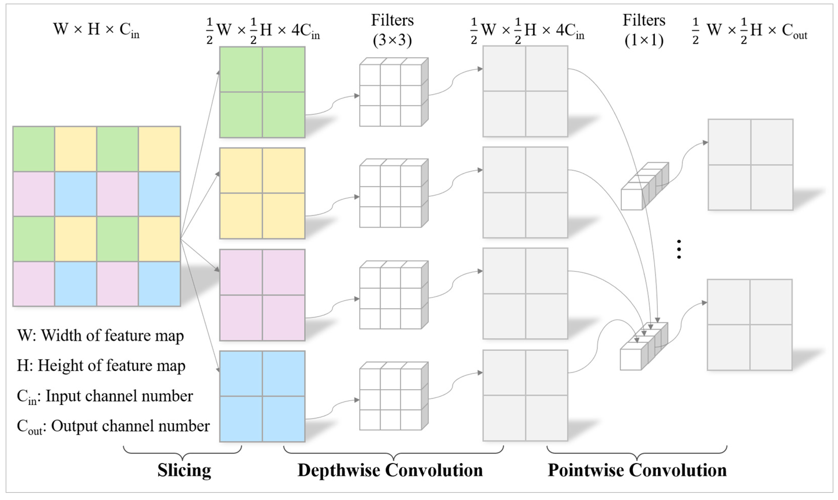
3.1. SliceSamp: The Downsampling Component

The SliceSamp component consists of two main layers: a slicing layer and a depthwise separable convolution layer including depthwise convolution and pointwise convolution, as shown in Figure 2. For each channel of the input feature map, we first obtain four sub-maps by slicing and then implement depthwise separable convolution on the four sub-maps. Slicing provides a means of implementing downsampling by reducing the dimensions of feature maps without increasing the number of model parameters. Subsequently, depthwise separable convolutions (DSConvs) can simultaneously capture the spatial and channel-wise features of the downsampled outputs, thereby ensuring timely learning and the effective extraction of image features.

To provide a clearer description of the designed neural network component, the pseudocode for the SliceSamp algorithm is provided in Algorithm 1:

Algorithm 1: output ← SliceSamp (X)

/* Performs downsampling on input features using the SliceSamp algorithm. */ Input: X$\in {ℝ}^{B\times C\times H\times W}$, vector representations of the input feature map, where B is the batch size, C is the dimension, H is the feature map height, and W is the feature map width. Output:  output $\in {ℝ}^{B\times C\times \frac{H}{2}\times \frac{W}{2}}$, updated vector representations after downsampling using SliceSamp. Parameters: Wdepthwise$\in {ℝ}^{{\mathrm{C}}_{\mathrm{in}}\times {\mathrm{C}}_{\mathrm{in}}\times \mathrm{K}\times \mathrm{K}}$, bdepthwise = 0 Wpointwise$\in {ℝ}^{{\mathrm{C}}_{\mathrm{in}}\times {\mathrm{C}}_{\mathrm{out}}\times 1\times 1}$, bpointwise = 0, where Cin is the number of input channels, Cout is the number of output channels, and K represents the spatial dimensions of each convolutional kernel. 1. X_slice ← [                                // Slice the input feature map         X [..., ::2, ::2],  // Upper-left corner         X [..., 1::2, ::2],   // Upper-right corner         X [..., ::2, 1::2],   // Lower-left corner         X [..., 1::2, 1::2]   // Lower-right corner              ] 2. X_concat ← concatenate (x_slice, axis=1)           // Merge slices in channel dimension 3. Depthwise_conv ← Wdepthwise * X_ concat + bdepthwise   // Depthwise Separable Convolution 4. Depthwise_bn ← BatchNormal (Depthwise_conv) 5. Depthwise_act ← GELU (Depthwise_bn) 6. Pointwise_conv ← Wpointwise * Depthwise_act + bpointwise 7. Pointwise_bn ← BatchNormal (Pointwise_conv) 8. output ← GELU (Pointwise_bn) 9. return output

In the slicing layer, four sub-maps are created by slicing each channel of the original feature map along the width and height dimensions with a stride of two, and the four sub-maps are then concatenated along the channel dimension. By slicing along the odd and even indexes on the spatial dimensions, respectively, the four sub-maps become half of the original feature map in both width and height, while the channel dimension is expanded to 4× the input size, and the other dimensions remain unchanged. It is interesting that the slicing operation achieves downsampling and retains all features only via a simple dimensional transformation.

In the depthwise separable convolution layer, a series of efficient convolution operations are employed for the concatenated sub-maps from the slicing layer. There are two main operations: depthwise convolution and pointwise convolution. For the depthwise convolution, the 3 × 3 filters, each with a padding of one, are employed to perform a stride of one convolution operation for each input channel separately, which produces a set of output channels with the same number as the slicing layer. Depthwise convolution is mainly used to capture the high-level semantic features in local regions without mixing the information of different channels. This operation reduces the computational complexity of the convolutional layers while efficiently extracting spatial information. In the second operation, pointwise convolution applies multiple 1 × 1 filters to combine the output channels from the depthwise convolution. This operation is used to mix information from different channels, encode channel importance, and capture correlations across channels. It allows for the flexible adjustment of the number of channels to suit subsequent operations such as convolution. The outputs from the depthwise and pointwise convolutions are fed to a Batch Normalization (BN) layer and a GELU (Gaussian Error Linear Unit) activation function, thus stabilizing the training process, reducing the effects of internal covariate shift, improving model generalization, and introducing nonlinearity. The combination of slicing and depthwise separable convolutions can reduce the number of parameters and computational costs in the downsampling process while retaining the full amount of feature information, achieving a good balance between model accuracy and inference speed.

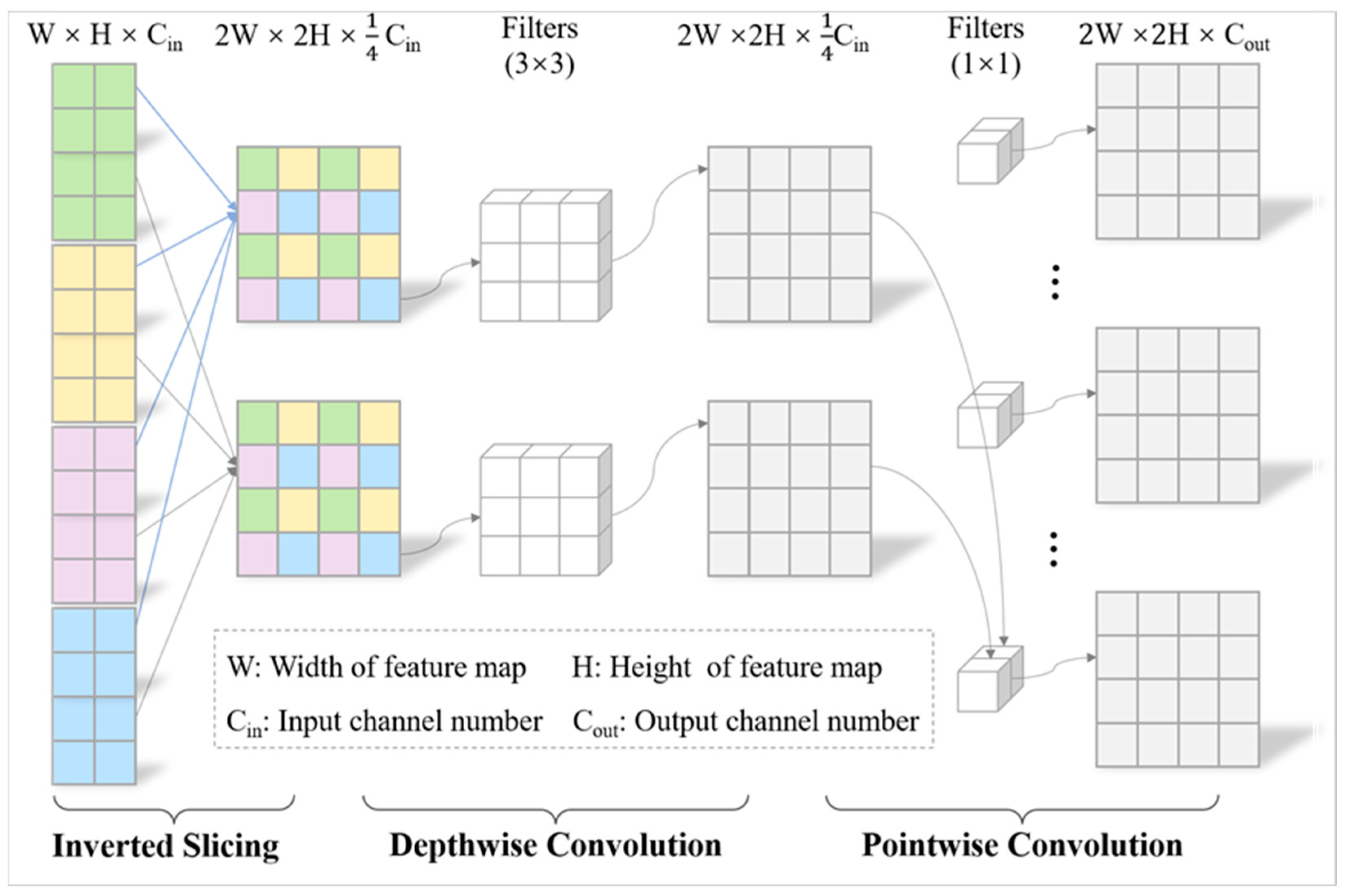
3.2. SliceUpsamp: The Upsampling Component

Most pooling-based and subsampling methods lack a mechanism of bidirectional mapping between the original feature maps and the sub-maps. This limitation makes it challenging to recover a refined high-resolution feature map. This is not friendly for fine-grained CV tasks such as semantic segmentation [21], small-object detection [57], and super-resolution [20]. Therefore, we propose a SliceUpsamp component for bi-directional mapping with SliceSamp which is based on inverted slicing and depthwise separable convolution.

Firstly, in the inverted slicing layer, the input features are equally divided into four group feature sets along the channel dimension, and they are then are rearranged into 2 × 2 nearest neighbor regions to obtain a high-resolution feature map, as shown in Figure 3. It can be seen that inverted slicing is a lossless feature reorganization process which directly transfers features from the channel dimension to the spatial dimension. At this stage, the width and height of feature maps are expanded to 2× the input size, while the channel dimension is reduced to 1/4 of the input size.

Finally, the high-resolution feature maps from the slicing layer are fed into the depthwise separable convolution layer to extract spatial information and capture the channel relationships. SliceUpsamp can reconstruct high-resolution features using position indexes in an orderly manner, thus achieving accurate matching and the alignment of the original feature map while ensuring upsampling efficiency. Given our aim of thoroughly learning image features with lower computational complexity, we accordingly minimize the parametrization in convolutional configurations. Specifically, in the SliceUpsamp module, we employ the same parameter setting as SliceSamp, utilizing 3 × 3 filters with a stride of one and a padding of one for depthwise convolution, as well as 1 × 1 convolutional kernels with a stride of one and zero padding for pointwise convolution.

4. Experiments

We conducted extensive experiments based on various deep learning architectures including ResNet [2], YOLOv5 [58], and Swin Transformer [32], and several benchmark datasets, including ImageNet-1K [59], Microsoft COCO (Common Objects in Context) [60], PASCAL VOC [61], and ADE20K [62], which cover a variety of CV tasks in image classification, object detection, and semantic segmentation. Below, we compare the proposed method with classical methods by replacing the downsampling layers in the above network architecture. Moreover, we also compare the algorithmic complexity of these methods, using the number of parameters as a measure of spatial complexity (i.e., memory), and FLOPs (Floating Point Operations) or MACs (Multiply–Accumulate Operations) as a measure of time complexity (i.e., computational latency).

4.1. Image Classification on ImageNet-1K

For the image classification task, we report the Top-1 and Top-5 accuracy values of several classical methods, including SoftPool [12], AdaPool [11], and Patch Merging [32], and our SliceSamp method based on an ImageNet-1K benchmark dataset, replacing the Max Pooling layer of the ResNet-18 [2] model with the aforementioned algorithms. Meanwhile, we also compare the number of parameters and time complexity of these models.

4.1.1. Image Classification Datasets

ImageNet-1K [59] is a large-scale dataset for image classification tasks which consists of a training set (1.28 million images) and a validation set (50,000 images). The images in this dataset were captured from various scenes and labeled into 1000 categories. As a benchmark, the dataset has been widely used for training and evaluating deep learning models and has played a crucial role in advancing the field of computer vision.

4.1.2. Experiment Setup

In the image classification experiment, ResNet-18 was treated as the baseline model. We evaluated classical downsampling methods on the ImageNet-1K dataset by replacing the Max Pooling layer in the baseline model. All these models were trained using a single GPU (Graphic Processing Unit) for 60 epochs with a learning rate reduction every 30 epochs, as our method has shown obvious advantages under the current epoch setting. We adopted an SGD (Stochastic Gradient Descent) optimizer with an initial learning rate of 0.1 and a weight decay of 0.0001. The other training configurations were uniformly set to a batch size of 256 and an image size of 224 × 224. In addition, we employed several data augmentation strategies, including randomly cropping spatial regions of a size of 299 × 299 pixels, resizing them to 224 × 224 pixels, and carrying out data normalization.

4.1.3. Results and Discussion

Table 1. The accuracy and computational cost of the models on ImageNet-1K.

Method	Model	Epoch	Batch Size	Image Size	Params	MACs	Top-1	Top-5
MaxPool (baseline)	ResNet-18	60	256	224	11.69 M	1.82 G	59.73	82.87
SoftPool	ResNet-18	60	256	224	11.69 M	1.82 G	59.77	82.86
AdaPool	ResNet-18	60	256	224	11.69 M	1.82G	59.38	82.56
Patch Merging	ResNet-18	60	256	224	11.71 M	1.87 G	41.36	66.95
SliceSamp (Ours)	ResNet-18	60	256	224	11.71 M	1.88 G	61.03	83.74

compares the Top-1, Top-5, and computational costs of various downsampling methods when performing the image classification task. When the model was trained with 60 epochs, our method outperformed other models by 1.26~19.67% of the Top-1 accuracy. SoftPool and AdaPool show similar accuracies to the baseline method MaxPool, yet they still exhibit significant performance gaps compared to our method. Additionally, Patch Merging shows lower model performance than the above three methods, which demonstrates that patch merging loses its effectiveness when applied to CNN (Convolutional Neural Network) architectures. In terms of computational cost, MaxPool, SoftPool, and AdaPool have roughly the same number of parameters and degree of computational complexity, while Patch Merging and our method are slightly higher in comparison. Compared to the baseline model, our method is only 3% higher with respect to MACs and 0.17% higher with respect to the number of parameters (Params in the following tables). It is worth noting that the levels of performance of most of the models are similar since only one Max Pooling layer is available for replacement in the ResNet-18 model, which has a relatively small impact on accuracy. However, our method can still improve Top-1 by 1.3% and Top-5 by 0.87% over the baseline. Experiments show that our method can significantly improve model performance with a similar algorithmic complexity by replacing the Max Pooling layer in the image classification task.

4.2. Object Detection on COCO and VOC

For the object detection task, we report the precision, recall, mean average precision (mAP@0.5), mAP@0.5:0.95, the number of parameters, and the computational complexity of several classical methods, including MaxPool, SoftPool, AdaPool, and Patch Merging, and our SliceSamp method based on two object detection benchmark datasets by replacing the Strided Convolution layers in the YOLOv5s-5.0 [58] model with the above algorithms. In addition, we also compare the convergence effect of different models while training them on the COCO [60] and VOC [61] datasets visually.

4.2.1. Object Detection Datasets

In the object detection experiments, we used two classic datasets, the Common Objects in Context (COCO) [60] and the Visual Object Classes (VOC) [61] datasets. Among these, the COCO dataset is a popular large-scale benchmark dataset which was designed for object detection and instance segmentation tasks. There are 80 object categories labeled in this dataset, and the annotations are provided in JSON (JavaScript Object Notation) format. The COCO dataset contains 118,287 training, 5000 validation, and 20,288 test-dev images with more than 2.5 million object instances. Moreover, the VOC dataset was first introduced in 2005 as part of the PASCAL (Pattern Analysis, Statistical Modelling, and Computational Learning) Visual Object Classes Challenge for the object detection task. It contains 20 object classes, and the annotations are provided in XML (eXtensible Markup Language) format. The VOC dataset has been updated and extended over the years, and the most recent version is VOC2012. The VOC dataset was obtained using the default code of the YOLOv5 algorithm, which includes 16,551 training and 4952 validation images.

4.2.2. Experiment Setup

In the object detection experiment, YOLOv5s-5.0 was treated as the baseline model. We evaluated classical downsampling methods on the COCO and VOC datasets by replacing the Strided Convolution layer in the baseline model. We replaced all Strided Convolution (Strided Conv) layers in the YOLOv5s-5.0 model, including four layers in the Backbone component and two layers in the Neck component. All models were trained using a single GPU for 300 epochs on the VOC dataset and 60 epochs on the COCO dataset. We adopted an SGD optimizer with an initial learning rate of 0.01 and a weight decay of 0.0005. The training used a batch size of 64 and an image size of 640 × 640. In addition, we employed various data augmentation strategies, such as mosaic, MixUp, affine transformation, color transformation, and random horizontal and vertical flipping. We also used overfitting prevention strategies, including a cosine decay learning rate scheduler and 1000 iterations of linear warm-up.

4.2.3. Results and Discussion

Table 2. The accuracy and computational cost of the models on the COCO and VOC datasets.

Method	Model	Params	FLOPs	COCO				VOC
				Precision	Recall	mAP@0.5	mAP@0.5:0.95	Precision	Recall	mAP@0.5	mAP@0.5:0.95
Strided Conv (baseline)	YOLOv5s-5.0	7.28 M	17.2 G	62.18	48.60	51.91	32.05	79.71	71.16	78.50	51.75
Maxpool	YOLOv5s-5.0	5.23 M	12.9 G	58.52	44.98	47.14	27.97	76.16	70.54	74.98	47.74
Softpool	YOLOv5s-5.0	5.23 M	12.9 G	6.92	1.11	0.57	0.32	15.17	11.75	4.95	1.98
Adapool	YOLOv5s-5.0	5.23 M	12.9 G	0.64	4.02	0.36	0.09	10.80	14.11	4.41	1.68
Patch Merging	YOLOv5s-5.0	6.00 M	14.6 G	0.06	0.003	0.002	0.002	0.64	8.05	0.26	0.05
SliceSamp (ours)	YOLOv5s-5.0	6.03 M	14.7 G	62.89	48.79	52.08	32.59	80.88	71.90	78.71	53.85
SliceUpsamp (ours)	YOLOv5s-5.0	6.06 M	14.8 G	65.43	46.85	51.72	32.45	79.7	72.99	79.29	53.95

compares the model performance and computational cost of various downsampling methods on the object detection task. The model performance of MaxPool is significantly lower than that of the baseline Strided Conv for all accuracy evaluation metrics. Unexpectedly, Softpool, Adapool, and Patch Merging exhibit lower accuracy values in the precision, recall, mAP@0.5, and mAP@0.5:0.95 metrics. By checking their losses during training, it was found that their loss values for both the training and validation sets gradually become NaN, leading to gradient explosion and a failure to converge. It can be seen that these methods have poor cross-model compatibility and portability and are not suitable for directly replacing Strided Conv in the baseline model. In contrast, the accuracy of SliceSamp was slightly improved on both the COCO and VOC datasets compared to the baseline model. By further replacing the Nearest Neighbor Upsampling layer in the baseline model, we also evaluated the effectiveness of the proposed upsampling method. When all models were trained for 60 epochs on the COCO dataset, SliceUpsamp showed similar performance to the SliceSamp model without replacing the upsampling component. When all models were sufficiently trained for 300 epochs on the VOC dataset, SliceUpsamp outperformed the SliceSamp model by about 0.6% in terms of mAP@0.5. It can be seen that after sufficient training, our proposed upsampling method can further achieve good performance gains.

Moreover, it is noteworthy that our proposed method maintains or slightly improves model performance while significantly reducing the computational cost. Compared to the baseline model Strided Conv, SliceSamp reduces the number of parameters by 17.17% and the number of FLOPs by 14.53%. Experiments show that our method can significantly reduce the number of parameters and computational costs while maintaining the original model performance in a neural network in which Strided Conv is the main downsampling component.

4.3. Semantic Segmentation on ADE20K

For the semantic segmentation task, we report the mIoU (Mean Intersection over Union) and mAcc (Mean Accuracy) of several classical methods, including MaxPool, SoftPool, and AdaPool, and our SliceSamp based on the ADE20K [62] benchmark dataset by replacing the Patch Merging layer of the Swin Transformer [32] model with the above algorithms. In addition, we also provide statistics such as the number of parameters and computational complexity of these models.

4.3.1. Semantic Segmentation Datasets

The ADE20K [62] dataset is a benchmark dataset for semantic segmentation tasks which contains large-scale images of indoor and outdoor scenes from various environments. Each image in the dataset is annotated with pixel-level segmentation labels, covering 150 object and scene categories and providing fine-grained information about the contents of each scene. The ADE20K dataset has a total of 25 K images of which 20,210 are used for training, 2000 for validation, and 3000 for testing.

4.3.2. Experiment Setup

In the semantic segmentation experiment, the Swin Transformer model in MMSegmentation [63] was treated as the baseline. We evaluated classical downsampling methods on the ADE20K dataset by replacing the Patch Merging layer in the baseline model. We replaced all Patch Merging layers employed in the last three downsampling operations of the Swin Transformer model. All models are trained on four GPUs for 160,000 iterations, with a linear warmup of 1500 iterations. We adopted the AdamW (adaptive moment estimation with decoupled weight decay) optimizer with an initial learning rate of 0.1 and a weight decay of 0.0001. The training configuration was uniformly set to assign two images per GPU with a batch size of eight and an image size of 512 × 512. In addition, we employed default data augmentation strategies, including random cropping, random flipping, and photometric distortion.

4.3.3. Results and Discussion

Table 3. The accuracy and computational cost of the models on ADE20K.

Method	Model	Iteration	Batch Size	Image Size	Params	FLOPs	mIoU	mAcc
Patch Merging (baseline)	Swin Transformer	160,000	8	224	59.94 M	236.1 G	21.99	30.75
Maxpool	Swin Transformer	160,000	8	224	58.78 M	235.4 G	23.08	32.50
Softpool	Swin Transformer	160,000	8	224	58.78 M	235.4 G	22.08	30.87
Adapool	Swin Transformer	160,000	8	224	58.78 M	235.4 G	20.95	29.13
SliceSamp (ours)	Swin Transformer	160,000	8	224	59.97 M	236.1 G	24.57	34.39

compares the mIoU, mAcc, and computational cost values of various downsampling methods on the semantic segmentation task. By replacing the Patch Merging layers in Swin Transformer, MaxPool and Softpool achieve slight accuracy improvements (+0.09~1.75%) in mIoU and mAcc metrics, respectively. However, Adapool suffers from accuracy degradation on the ADE20K dataset, showing less stability than MaxPool. Compared with MaxPool and Softpool, the SliceSamp model demonstrates further performance improvement. Compared to the baseline model, our model exhibits more significant performance gains of 2.58% in the mIoU and 3.64% in the mAcc. In terms of algorithmic complexity, Maxpool, Softpool, and Adapool have similar numbers of parameters and time complexities, yet their accuracy is lower than that of our method. Compared to the baseline model Patch Merging, our method increases the number of parameters by only 0.05% with the same FLOPs. Experiments show that our method can significantly improve model performance with similar algorithmic complexity in neural networks in which Patch Merging is the main downsampling component.

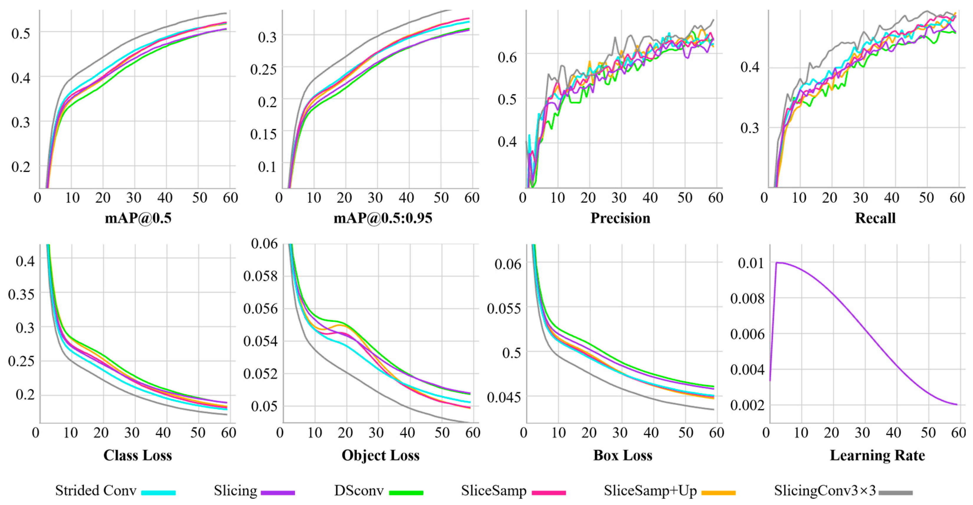
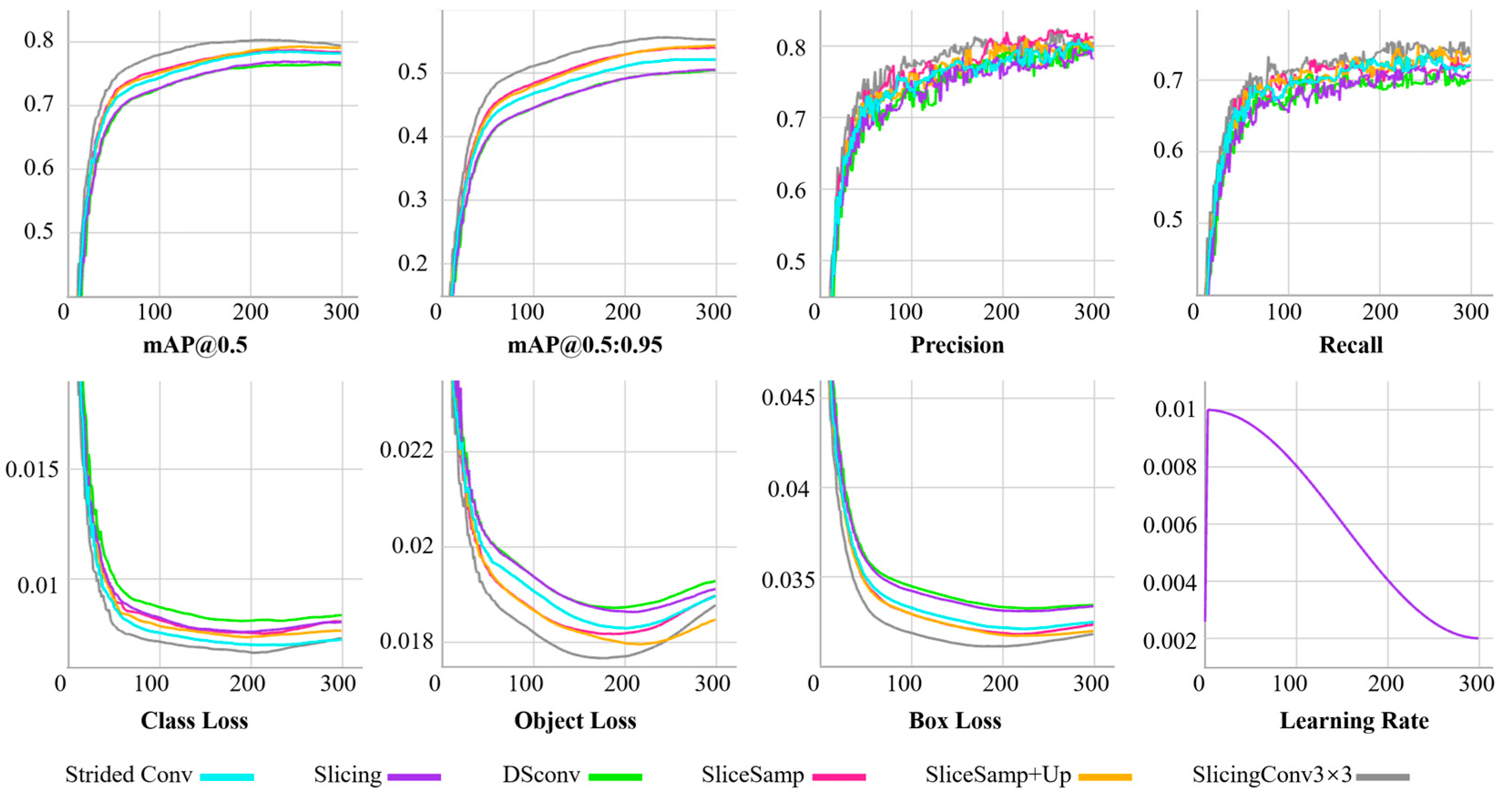
4.4. Ablation Studies

In this section, we perform extensive experiments to analyze the important design elements in the proposed method, including slicing, DSConv, and upsampling components (+Up, in the following table). We discuss the balanced capability of the proposed approach in terms of algorithmic complexity and model performance. In addition, we visualize the process of training the models using different design elements.

4.4.1. Experiment Setup

Since the YOLOv5s-5.0 [58] model architecture is easy to modify and trains quickly, we chose it to conduct ablation experiments with different design elements. Also, we used the same datasets and experimental settings as in Section 4.2 for the object detection task. We ablated slicing and DSConv by replacing the Strided Conv layers and investigate the gain in performance of adding the SliceUpsamp component (+Up) by replacing the Nearest Neighbor Upsampling layers. Specifically, the Slicing method uses only a slicing layer to downsample and a 1 × 1 convolution to transform the channel dimension. The DSConv method uses only a DSConv with a stride of two to downsample and transform the channel dimension. The SliceSamp method uses both the slicing downsampling and DSConv design elements. The SliceUpSamp method further uses the SliceUpsamp component to replace the Nearest Neighbor Upsampling layer of the SliceSamp method. The SlicingConv3×3 method uses a slicing layer to downsample and a 3 × 3 convolution to transform the channel dimension and extract feature information.

4.4.2. Results and Discussion

Table 4. Ablation study on COCO and VOC benchmarks based on the YOLOv5 model.

Method	Slicing	DSConv	+Up	Params	FLOPs	COCO				VOC
						Precision	Recall	mAP@0.5	mAP@0.5:0.95	Precision	Recall	mAP@0.5	mAP@0.5:0.95
Strided Conv (baseline)	-	-	-	7.28 M	17.2 G	62.18 (+0.00)	48.60 (+0.00)	51.91 (+0.00)	32.05 (+0.00)	79.71 (+0.00)	71.16 (+0.00)	78.50 (+0.00)	51.75 (+0.00)
Slicing	√	-	-	6.00 M	14.5 G	63.48 (+1.30)	45.99 (−2.61)	50.65 (−1.26)	30.76 (−1.29)	76.93 (−2.78)	71.69 (+0.53)	76.95 (−1.55)	49.92 (−1.83)
DSConv	-	√	-	5.24 M	13.0 G	63.49 (+1.31)	45.78 (−2.82)	50.54 (−1.37)	30.96 (−1.09)	78.85 (−0.86)	70.15 (−1.01)	76.54 (−1.96)	50.22 (−1.53)
SliceSamp (ours)	√	√	-	6.03 M	14.7 G	62.89 (+0.71)	48.79 (+0.19)	52.08 (+0.17)	32.59 (+0.54)	80.88 (+1.17)	71.90 (+0.74)	78.71 (+0.21)	53.85 (+2.10)
SliceUpSamp (ours)	√	√	√	6.06 M	14.8 G	65.43 (+3.25)	46.85 (−1.75)	51.72 (−0.19)	32.45 (+0.40)	79.70 (−0.01)	72.99 (+1.83)	79.29 (+0.79)	53.95 (+2.20)
SlicingConv3×3	√	-	-	15.50 M	33.0 G	67.64 (+5.46)	48.37 (−0.23)	54.08 (+2.17)	34.60 (+2.01)	78.49 (−1.22)	75.02 (+3.86)	80.32 (+1.82)	55.17 (+3.42)

shows the ablation detail, algorithm complexity, and model performance for different design elements. In this table, red text indicates a decrease in performance relative to the baseline, while green text indicates an improvement in performance relative to the baseline. “√” indicates that the current design element is considered in the model.

On both the COCO and VOC datasets, the Slicing and DSConv methods exhibited poor performance with respect to various accuracy metrics. Although the DSConv method demonstrated a slight performance improvement compared to the Slicing method on the VOC dataset, it still has a large gap in accuracy between both Strided Conv and our method. This indicates that using only a single design element does not achieve good model performance. When considering both slicing and DSConv, SliceSamp achieved a slightly better performance than Strided Conv while reducing the number of parameters by 17.17% and the number of FLOPS by 14.53%. By further replacing the Nearest Neighbor Upsampling layers in SliceSamp, the SliceUpSamp method outperformed the SliceSamp method by 0.58% mAP@0.5 on the VOC dataset while achieving similar performance on the COCO dataset. This indicates that the proposed upsampling component can further improve model performance when sufficient model training cycles are available. Finally, we also tested the impact of the SlicingConv3×3 method with a higher degree of algorithmic complexity on the model’s performance. We found that a higher degree of model accuracy can be achieved using a combination of slicing layers and Conv3×3. However, the disadvantage is that this required sacrificing a large amount of computational cost. Compared with our method, the SlicingConv3×3 method increased the number of parameters by 157% and the FLOPs by 124%. The results show that our proposed SliceSamp method has significant advantages in terms of balancing model performance and algorithm complexity. It can achieve a higher degree of model accuracy at a lower computational cost.

To investigate the impact of various design elements on model performance, we employed Gradient-weighted Class Activation Mapping (Grad-CAM) [64] to generate heatmaps for different object categories. The heatmaps produced via Grad-CAM revealed the model’s attention distribution, helping us understand the feature mapping within the neural network. In this context, color intensity signifies the model’s degree of focus on different regions of the input image, with the color becoming redder, indicating the greater significance of those features for the model’s predictions. Figure 4 visualizes the Grad-CAM heatmaps for different design elements across different methods.

In Figure 4, the top row displays heatmaps for the “Person” category. Most algorithms exhibited good attention toward the “Person” category, with our proposed methods demonstrating larger attention regions. The second row showcases heatmaps for the “Horse” category in which the Strided Conv and Slicing methods tended to focus on the horse’s abdominal region, while other methods encompassed a wider area, including the front hooves and tail. The third row exhibits heatmaps for multiple instances of the “Person” category, with the Slicing and DSConv methods displaying comparatively lower attention levels while other methods generally yielded satisfactory results. The fourth row presents heatmaps for the “Bus” category in which Slicing and DSConv tended to focus on unrelated areas, resulting in less robust performance in this category compared to our proposed methods. In summary, compared to our proposed model, models employing a single design element exhibited slightly inferior performance in terms of attention distribution areas and focus intensity. This can impact a model’s precision and recall, thereby leading to a decrease in the model’s overall performance.

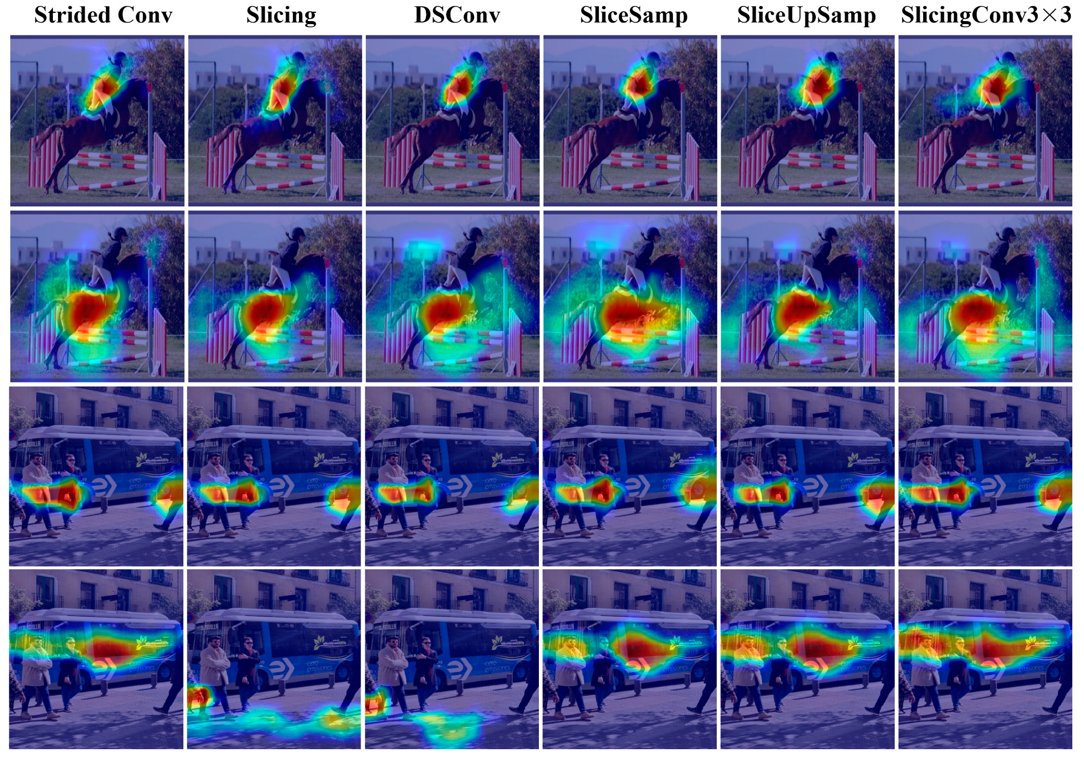
4.4.3. Visual Comparison

In this section, based on the COCO dataset, the validation accuracy and loss changes were visually compared during the process of training models with different design elements, as shown in Figure 5. From the mAP@0.5 and mAP@0.5:0.95 metrics, it is clear that the models with different design elements exhibit three different levels of model performance. The Slicing and DSConv methods, each with only a single design element, are at the lowest level of model accuracy. The proposed SliceSamp and SliceUpsamp methods, with both slicing and DSConv elements, perform similarly to Strided Conv and show a trend of further improvement after the 50th epoch. The SlicingConv3×3 method, which combines Slicing and 3 × 3 convolution, achieves the highest model performance yet, as mentioned before, it is more computationally expensive. In terms of the loss changes on the validation set, the loss values of all models also converged to three levels. All models showed a pattern of lower loss values with higher mAP values. However, it is noteworthy that the proposed method converges to lower loss values on Object loss after the 40th epoch, which is similar to the Strided Conv method on Class and Box losses. It can be seen that our method has better generalization compared to the baseline Strided Conv.

Meanwhile, based on the VOC dataset, the validation accuracy and loss changes were visually compared during model training with 300 epochs, as shown in Figure 6. As seen from the mAP@0.5 and mAP@0.5:0.95 metrics, the Slicing and DSConv methods still exhibit the lowest model accuracy. Although the SlicingConv3×3 method achieves the highest model performance, the validation accuracy gradually decreases and exhibits overfitting after the 200th epoch. However, the accuracy of the proposed SliceSamp and SliceUpsamp methods continues to steadily improve after the 200th epoch. In particular, in terms of the mAP@0.5:0.95 metric, our method is significantly higher than the Strided Conv method after the 50th epoch. In terms of loss convergence on the validation set, on the Class, Object, and Box losses, both the Slicing and DSConv methods converge to higher values, and the SlicingConv3×3 method converges to lower values. Although our methods (SliceSamp and SliceUpsamp) have slightly higher Class loss values than Strided Conv, they converge to lower loss values on the Object and Box losses. It is noteworthy that SliceUpsamp exhibits loss values close to those of the SlicingConv3×3 method on the Object and Box losses after the 250th epoch. Moreover, when SlicingConv3×3 is overfitting on Object loss, SliceUpsamp still maintains a low loss value, showing good robustness.

5. Discussion

Our approach enables seamless integration into both CNN-based and Transformer-based models, thereby achieving a more favorable balance between algorithmic complexity and model performance. However, certain limitations may hinder its broader adoption in specific application scenarios. Firstly, our components were founded on the CNN architecture, which may not confer a distinct advantage in cases in which researchers prefer to construct neural networks exclusively based on the Transformer architecture. Nevertheless, it is noteworthy that the existing research has demonstrated that hybrid networks incorporating both CNN and Transformer architectures can yield substantial performance gains. Secondly, CNN-based components tend to emphasize local attention, leaving room for improvement in their capacity to capture global context. Therefore, in future work, we intend to explore the development of efficient downsampling components grounded in the Transformer architecture.

6. Conclusions

In this paper, we introduce SliceSamp, an effective downsampling method that enhances model performance while minimizing computational latency and memory requirements. To reconstruct and align high-resolution feature maps, we also developed SliceUpsamp for upsampling, employing inverted slicing and depthwise separable convolution. We validated the effectiveness of SliceSamp across multiple datasets, including ImageNet-1K, COCO, VOC, and ADE20K. Extensive experiments demonstrate SliceSamp’s superior performance across various computer vision tasks compared to other classical downsampling methods. Compared with the baseline model, SliceSamp improves Top-1 by 1.3% and Top-5 by 0.87% on the image classification task, maintains a similar accuracy while reducing the number of parameters by 17.17% and FLOPs by 14.53% on the object detection task, and improves mIoU by 2.58% and mAcc by 3.64% on the semantic segmentation task. In addition, ablation studies and a Grad-CAM analysis show that integrating Slicing and DSConv can provide a qualitative leap in model performance compared to the use of a single element. SliceSamp seamlessly integrates into various models like ResNet, YOLO, and Transformer. We firmly believe that SliceSamp represents a superior and promising alternative to widely used downsampling methods.

References

1. LeCun, Y.; Bengio, Y.; Hinton, G. Deep learning. Nature 2015, 521, 436–444. [Google Scholar] [CrossRef]
2. He, K.; Zhang, X.; Ren, S.; Sun, J. Deep residual learning for image recognition. In Proceedings of the IEEE Computer Society Conference on Computer Vision and Pattern Recognition (CVPR), Las Vegas, NV, USA, 27–30 June 2016; pp. 770–778. [Google Scholar] [CrossRef]
3. He, K.; Gkioxari, G.; Dollar, P.; Girshick, R. Mask R-CNN. In Proceedings of the IEEE International Conference on Computer Vision, Venice, Italy, 22–29 October 2017; pp. 2961–2969. Available online: https://openaccess.thecvf.com/content_iccv_2017/html/He_Mask_R-CNN_ICCV_2017_paper.html (accessed on 20 October 2023).
4. Redmon, J.; Divvala, S.; Girshick, R.; Farhadi, A. You Only Look Once: Unified, Real-Time Object Detection. In Proceedings of the 2016 IEEE Conference on Computer Vision and Pattern Recognition (CVPR), Las Vegas, NV, USA, 27–30 June 2016; pp. 779–788. [Google Scholar] [CrossRef]
5. Ronneberger, O.; Fischer, P.; Brox, T. U-Net: Convolutional Networks for Biomedical Image Segmentation. In Medical Image Computing and Computer-Assisted Intervention—MICCAI 2015; Navab, N., Hornegger, J., Wells, W., Frangi, A., Eds.; Springer International Publishing: Cham, Switzerland, 2015; pp. 234–241. [Google Scholar] [CrossRef]
6. Sinha, R.K.; Pandey, R.; Pattnaik, R. Deep Learning for Computer Vision Tasks: A review. arXiv 2018, arXiv:1804.03928. [Google Scholar] [CrossRef]
7. Shi, W.; Cao, J.; Zhang, Q.; Li, Y.; Xu, L. Edge Computing: Vision and Challenges. IEEE Internet Things J. 2016, 3, 637–646. [Google Scholar] [CrossRef]
8. Shen, S.; Li, R.; Zhao, Z.; Liu, Q.; Liang, J.; Zhang, H. Efficient Deep Structure Learning for Resource-Limited IoT Devices. In Proceedings of the GLOBECOM 2020–2020 IEEE Global Communications Conference, Taipei, Taiwan, 7–11 December 2020; pp. 1–6. [Google Scholar] [CrossRef]
9. Xie, Y.; Guo, Y.; Mi, Z.; Yang, Y.; Obaidat, M.S. Edge-Assisted Real-Time Instance Segmentation for Resource-Limited IoT Devices. IEEE Internet Things J. 2023, 10, 473–485. [Google Scholar] [CrossRef]
10. Voulodimos, A.; Doulamis, N.; Doulamis, A.; Protopapadakis, E. Deep Learning for Computer Vision: A Brief Review. Comput. Intell. Neurosci. 2018, 2018, e7068349. [Google Scholar] [CrossRef] [PubMed]
11. Stergiou, A.; Poppe, R. AdaPool: Exponential Adaptive Pooling for Information-Retaining Downsampling. IEEE Trans. Image Process. 2023, 32, 251–266. [Google Scholar] [CrossRef] [PubMed]
12. Stergiou, A.; Poppe, R.; Kalliatakis, G. Refining Activation Downsampling with SoftPool. In Proceedings of the IEEE/CVF International Conference on Computer Vision, Montreal, QC, Canada, 10–17 October 2021; pp. 10357–10366. Available online: https://openaccess.thecvf.com/content/ICCV2021/html/Stergiou_Refining_Activation_Downsampling_With_SoftPool_ICCV_2021_paper.html (accessed on 20 October 2023).
13. Zhai, S.; Wu, H.; Kumar, A.; Cheng, Y.; Lu, Y.; Zhang, Z.; Feris, R. S3Pool: Pooling with Stochastic Spatial Sampling. In Proceedings of the IEEE Conference on Computer Vision and Pattern Recognition, Honolulu, HI, USA, 21–26 July 2017; pp. 4970–4978. Available online: https://openaccess.thecvf.com/content_cvpr_2017/html/Zhai_S3Pool_Pooling_With_CVPR_2017_paper.html (accessed on 20 October 2023).
14. Akhtar, N.; Ragavendran, U. Interpretation of intelligence in CNN-pooling processes: A methodological survey. Neural Comput. Appl. 2020, 32, 879–898. [Google Scholar] [CrossRef]
15. Ajani, T.S.; Imoize, A.L.; Atayero, A.A. An Overview of Machine Learning within Embedded and Mobile Devices–Optimizations and Applications. Sensors 2021, 21, 4412. [Google Scholar] [CrossRef]
16. Ayachi, R.; Afif, M.; Said, Y.; Atri, M. Strided Convolution Instead of Max Pooling for Memory Efficiency of Convolutional Neural Networks. In Proceedings of the 8th International Conference on Sciences of Electronics, Technologies of Information and Telecommunications (SETIT’18), Genoa, Italy, 18–20 December 2018; Bouhlel, M., Rovetta, S., Eds.; Springer International Publishing: Cham, Switzerland, 2020; Volume 1, pp. 234–243. [Google Scholar] [CrossRef]
17. Devi, N.; Borah, B. Cascaded pooling for Convolutional Neural Networks. In Proceedings of the 2018 Fourteenth International Conference on Information Processing (ICINPRO), Bangalore, India, 21–23 December 2018; pp. 1–5. [Google Scholar]
18. Kuen, J.; Kong, X.; Lin, Z.; Wang, G.; Yin, J.; See, S.; Tan, Y.-P. Stochastic Downsampling for Cost-Adjustable Inference and Improved Regularization in Convolutional Networks. In Proceedings of the IEEE Conference on Computer Vision and Pattern Recognition, Salt Lake City, UT, USA, 18–23 June 2018; pp. 7929–7938. Available online: https://openaccess.thecvf.com/content_cvpr_2018/html/Kuen_Stochastic_Downsampling_for_CVPR_2018_paper.html (accessed on 20 October 2023).
19. Saeedan, F.; Weber, N.; Goesele, M.; Roth, S. Detail-Preserving Pooling in Deep Networks. In Proceedings of the IEEE Conference on Computer Vision and Pattern Recognition, Salt Lake City, UT, USA, 18–23 June 2018; pp. 9108–9116. Available online: https://openaccess.thecvf.com/content_cvpr_2018/html/Saeedan_Detail-Preserving_Pooling_in_CVPR_2018_paper.html (accessed on 20 October 2023).
20. Yan, Y.; Liu, C.; Chen, C.; Sun, X.; Jin, L.; Peng, X.; Zhou, X. Fine-Grained Attention and Feature-Sharing Generative Adversarial Networks for Single Image Super-Resolution. IEEE Trans. Multimed. 2022, 24, 1473–1487. [Google Scholar] [CrossRef]
21. Lin, G.; Milan, A.; Shen, C.; Reid, I. RefineNet: Multi-path Refinement Networks for High-Resolution Semantic Segmentation. In Proceedings of the IEEE Conference on Computer Vision and Pattern Recognition (CVPR), Honolulu, HI, USA, 21–26 July 2017; pp. 5168–5177. [Google Scholar] [CrossRef]
22. Gragnaniello, D.; Cozzolino, D.; Marra, F.; Poggi, G.; Verdoliva, L. Are GAN Generated Images Easy to Detect? A Critical Analysis of the State-Of-The-Art. In Proceedings of the 2021 IEEE International Conference on Multimedia and Expo (ICME), Shenzhen, China, 5–9 July 2021; pp. 1–6. [Google Scholar] [CrossRef]
23. Li, Y.; Cai, W.; Gao, Y.; Li, C.; Hu, X. More than Encoder: Introducing Transformer Decoder to Upsample. In Proceedings of the 2022 IEEE International Conference on Bioinformatics and Biomedicine (BIBM), Las Vegas, NV, USA, 6–8 December 2022; pp. 1597–1602. [Google Scholar] [CrossRef]
24. Fadnavis, S. Image Interpolation Techniques in Digital Image Processing: An Overview. Int. J. Eng. Res. Appl. 2014, 4, 2248–962270. [Google Scholar]
25. Zeiler, M.D.; Taylor, G.W.; Fergus, R. Adaptive deconvolutional networks for mid and high level feature learning. In Proceedings of the 2011 IEEE International Conference on Computer Vision, Barcelona, Spain, 6–13 November 2011; pp. 2018–2025. [Google Scholar] [CrossRef]
26. Shi, W.; Caballero, J.; Huszár, F.; Totz, J.; Aitken, A.P.; Bishop, R.; Rueckert, D.; Wang, Z. Real-Time Single Image and Video Super-Resolution Using an Efficient Sub-Pixel Convolutional Neural Network. In Proceedings of the IEEE Conference on Computer Vision and Pattern Recognition, Las Vegas, NV, USA, 27–30 June 2016; pp. 1874–1883. Available online: https://www.cv-foundation.org/openaccess/content_cvpr_2016/html/Shi_Real-Time_Single_Image_CVPR_2016_paper.html (accessed on 20 October 2023).
27. Olivier, R.; Hanqiang, C. Nearest Neighbor Value Interpolation. Int. J. Adv. Comput. Sci. Appl. 2012, 3, 25–30. [Google Scholar] [CrossRef]
28. Hwang, J.W.; Lee, H.S. Adaptive Image Interpolation Based on Local Gradient Features. IEEE Signal Process. Lett. 2004, 11, 359–362. [Google Scholar] [CrossRef]
29. Zhong, F.; Li, M.; Zhang, K.; Hu, J.; Liu, L. DSPNet: A low computational-cost network for human pose estimation. Neurocomputing 2021, 423, 327–335. [Google Scholar] [CrossRef]
30. Zeiler, M.D.; Fergus, R. Stochastic Pooling for Regularization of Deep Convolutional Neural Networks. arXiv 2013, arXiv:1301.3557. [Google Scholar] [CrossRef]
31. Dosovitskiy, A.; Beyer, L.; Kolesnikov, A.; Weissenborn, D.; Zhai, X.; Unterthiner, T.; Dehghani, M.; Minderer, M.; Heigold, G.; Gelly, S.; et al. An Image Is Worth 16 × 16 Words: Transformers for Image Recognition at Scale. arXiv 2021, arXiv:2010.11929. Available online: http://arxiv.org/abs/2010.11929 (accessed on 20 October 2023).
32. Liu, Z.; Lin, Y.; Cao, Y.; Hu, H.; Wei, Y.; Zhang, Z.; Lin, S.; Guo, B. Swin Transformer: Hierarchical Vision Transformer Using Shifted Windows. In Proceedings of the IEEE/CVF International Conference on Computer Vision, Montreal, BC, Canada, 11–17 October 2021; pp. 10012–10022. Available online: https://openaccess.thecvf.com/content/ICCV2021/html/Liu_Swin_Transformer_Hierarchical_Vision_Transformer_Using_Shifted_Windows_ICCV_2021_paper.html (accessed on 20 October 2023).
33. Gao, Z.; Wang, L.; Wu, G. LIP: Local Importance-Based Pooling. In Proceedings of the IEEE/CVF International Conference on Computer Vision, Seoul, Republic of Korea, 27 October–2 November 2019; pp. 3355–3364. Available online: https://openaccess.thecvf.com/content_ICCV_2019/html/Gao_LIP_Local_Importance-Based_Pooling_ICCV_2019_paper.html (accessed on 20 October 2023).
34. Yu, D.; Wang, H.; Chen, P.; Wei, Z. Mixed Pooling for Convolutional Neural Networks. In Rough Sets and Knowledge Technology; Miao, D., Pedrycz, W., Ślȩzak, D., Peters, G., Hu, Q., Wang, R., Eds.; Springer International Publishing: Cham, Switzerland, 2014; pp. 364–375. [Google Scholar] [CrossRef]
35. Wu, Y.-H.; Liu, Y.; Zhan, X.; Cheng, M.-M. P2T: Pyramid Pooling Transformer for Scene Understanding. IEEE Trans. Pattern Anal. Mach. Intell. 2022, 45, 12760–12771. [Google Scholar] [CrossRef]
36. Graham, B. Fractional Max-Pooling. arXiv 2015. [Google Scholar] [CrossRef]
37. Sun, M.; Song, Z.; Jiang, X.; Pan, J.; Pang, Y. Learning Pooling for Convolutional Neural Network. Neurocomputing 2017, 224, 96–104. [Google Scholar] [CrossRef]
38. Montavon, G.; Lapuschkin, S.; Binder, A.; Samek, W.; Müller, K.-R. Explaining nonlinear classification decisions with deep Taylor decomposition. Pattern Recognit. 2017, 65, 211–222. [Google Scholar] [CrossRef]
39. Liu, Y.; Gross, L.; Li, Z.; Li, X.; Fan, X.; Qi, W. Automatic Building Extraction on High-Resolution Remote Sensing Imagery Using Deep Convolutional Encoder-Decoder with Spatial Pyramid Pooling. IEEE Access 2019, 7, 128774–128786. [Google Scholar] [CrossRef]
40. Redmon, J.; Farhadi, A. YOLO9000: Better, Faster, Stronger. arXiv 2016, arXiv:1612.08242. Available online: http://arxiv.org/abs/1612.08242 (accessed on 20 October 2023).
41. Khan, S.; Naseer, M.; Hayat, M.; Zamir, S.W.; Khan, F.S.; Shah, M. Transformers in Vision: A Survey. ACM Comput. Surv. 2022, 54, 1–41. [Google Scholar] [CrossRef]
42. Li, Y.; Liu, Z.; Wang, H.; Song, L. A Down-sampling Method Based on The Discrete Wavelet Transform for CNN Classification. In Proceedings of the 2023 2nd International Conference on Big Data, Information and Computer Network (BDICN), Xishuangbanna, China, 6–8 January 2023; pp. 126–129. [Google Scholar]
43. Lu, W.; Chen, S.-B.; Tang, J.; Ding, C.H.Q.; Luo, B. A Robust Feature Downsampling Module for Remote-Sensing Visual Tasks. IEEE Trans. Geosci. Remote. Sens. 2023, 61, 1–12. [Google Scholar] [CrossRef]
44. Ma, J.; Gu, X. Scene image retrieval with siamese spatial attention pooling. Neurocomputing 2020, 412, 252–261. [Google Scholar] [CrossRef]
45. Hesse, R.; Schaub-Meyer, S.; Roth, S. Content-Adaptive Downsampling in Convolutional Neural Networks. In Proceedings of the 2023 IEEE/CVF Conference on Computer Vision and Pattern Recognition Workshops (CVPRW), Vancouver, BC, Canada, 17–24 June 2023; pp. 4544–4553. [Google Scholar]
46. Zhao, J.; Snoek, C.G.M. LiftPool: Bidirectional ConvNet Pooling. arXiv 2021, arXiv:2104.00996. [Google Scholar] [CrossRef]
47. Chollet, F. Xception: Deep Learning with Depthwise Separable Convolutions. In Proceedings of the IEEE Conference on Computer Vision and Pattern Recognition, Honolulu, HI, USA, 21–26 July 2017; pp. 1251–1258. Available online: https://openaccess.thecvf.com/content_cvpr_2017/html/Chollet_Xception_Deep_Learning_CVPR_2017_paper.html (accessed on 20 October 2023).
48. Kaiser, L.; Gomez, A.N.; Chollet, F. Depthwise Separable Convolutions for Neural Machine Translation. arXiv 2017, arXiv:1706.03059. [Google Scholar] [CrossRef]
49. Liu, B.; Zou, D.; Feng, L.; Feng, S.; Fu, P.; Li, J. An FPGA-Based CNN Accelerator Integrating Depthwise Separable Convolution. Electronics 2019, 8, 281. [Google Scholar] [CrossRef]
50. Howard, A.G.; Zhu, M.; Chen, B.; Kalenichenko, D.; Wang, W.; Weyand, T.; Andreetto, M.; Adam, H. MobileNets: Efficient Convolutional Neural Networks for Mobile Vision Applications. arXiv 2017, arXiv:1704.04861. [Google Scholar] [CrossRef]
51. Drossos, K.; Mimilakis, S.I.; Gharib, S.; Li, Y.; Virtanen, T. Sound Event Detection with Depthwise Separable and Dilated Convolutions. In Proceedings of the 2020 International Joint Conference on Neural Networks (IJCNN), Glasgow, UK, 19–24 July 2020; pp. 1–7. [Google Scholar]
52. Zhang, X.; Zhou, X.; Lin, M.; Sun, J. ShuffleNet: An Extremely Efficient Convolutional Neural Network for Mobile Devices. In Proceedings of the IEEE Conference on Computer Vision and Pattern Recognition, Salt Lake City, UT, USA, 18–23 June 2018; pp. 6848–6856. Available online: https://openaccess.thecvf.com/content_cvpr_2018/html/Zhang_ShuffleNet_An_Extremely_CVPR_2018_paper.html (accessed on 20 October 2023).
53. Liu, F.; Xu, H.; Qi, M.; Liu, D.; Wang, J.; Kong, J. Depth-Wise Separable Convolution Attention Module for Garbage Image Classification. Sustainability 2022, 14, 3099. [Google Scholar] [CrossRef]
54. Pilipovic, R.; Bulic, P.; Risojevic, V. Compression of convolutional neural networks: A short survey. In Proceedings of the 2018 17th International Symposium INFOTEH-JAHORINA (INFOTEH), East Sarajevo, Bosnia and Herzegovina, 21–23 March 2018; pp. 1–6. [Google Scholar]
55. Winoto, A.S.; Kristianus, M.; Premachandra, C. Small and Slim Deep Convolutional Neural Network for Mobile Device. IEEE Access 2020, 8, 125210–125222. [Google Scholar] [CrossRef]
56. Elordi, U.; Unzueta, L.; Arganda-Carreras, I.; Otaegui, O. How Can Deep Neural Networks Be Generated Efficiently for Devices with Limited Resources? In Articulated Motion and Deformable Objects; Perales, F., Kittler, J., Eds.; Springer International Publishing: Cham, Switzerland, 2018; pp. 24–33. [Google Scholar] [CrossRef]
57. Sun, X.; Wang, P.; Yan, Z.; Xu, F.; Wang, R.; Diao, W.; Chen, J.; Li, J.; Feng, Y.; Xu, T.; et al. FAIR1M: A benchmark dataset for fine-grained object recognition in high-resolution remote sensing imagery. ISPRS J. Photogramm. Remote. Sens. 2022, 184, 116–130. [Google Scholar] [CrossRef]
58. ultralytics/yolov5: v5.0—YOLOv5-P6 1280 Models, AWS, Supervise.ly and YouTube Integrations. Available online: https://zenodo.org/record/4679653 (accessed on 11 April 2021).
59. Russakovsky, O.; Deng, J.; Su, H.; Krause, J.; Satheesh, S.; Ma, S.; Huang, Z.; Karpathy, A.; Khosla, A.; Bernstein, M.; et al. ImageNet Large Scale Visual Recognition Challenge. Int. J. Comput. Vis. 2015, 115, 211–252. [Google Scholar] [CrossRef]
60. Lin, T.Y.; Maire, M.; Belongie, S.; Bourdev, L.; Girshick, R.; Hays, J.; Perona, P.; Zitnick, C.L.; Dollár, P. Microsoft COCO: Common Objects in Context. In Computer Vision—ECCV 2014; Fleet, D., Pajdla, T., Schiele, B., Tuytelaars, T., Eds.; Springer International Publishing: Cham, Switzerland, 2014; pp. 740–755. [Google Scholar] [CrossRef]
61. Everingham, M.; Eslami, S.M.A.; Van Gool, L.; Williams, C.K.I.; Winn, J.; Zisserman, A. The Pascal Visual Object Classes Challenge: A Retrospective. Int. J. Comput. Vis. 2014, 111, 98–136. [Google Scholar] [CrossRef]
62. Zhou, B.; Zhao, H.; Puig, X.; Xiao, T.; Fidler, S.; Barriuso, A.; Torralba, A. Semantic Understanding of Scenes Through the ADE20K Dataset. Int. J. Comput. Vis. 2018, 127, 302–321. [Google Scholar] [CrossRef]
63. MMSegmentation Contributors. OpenMMLab Semantic Segmentation Toolbox and Benchmark. Available online: https://github.com/open-mmlab/mmsegmentation (accessed on 11 April 2023).
64. Selvaraju, R.R.; Cogswell, M.; Das, A.; Vedantam, R.; Parikh, D.; Batra, D. Grad-CAM: Visual Explanations from Deep Networks via Gradient-based Localization. Int. J. Comput. Vis. 2020, 128, 336–359. [Google Scholar] [CrossRef]
Figure 1. Feature information retained by different downsampling methods.
Applsci 13 11657 g001
Figure 2. The architecture of the SliceSamp component.
Applsci 13 11657 g002
Figure 3. The architecture of the SliceUpsamp component.
Applsci 13 11657 g003
Figure 4. Grad-CAM heatmaps for Different Design Elements.
Applsci 13 11657 g004
Figure 5. Validation accuracy and loss on the COCO dataset during model training.
Applsci 13 11657 g005
Figure 6. Validation accuracy and loss on the VOC dataset during model training.
Applsci 13 11657 g006