Article

Calibration of Viscous Damping–Stiffness Control Force in Active and Semi-Active Tuned Mass Dampers for Reduction of Harmonic Vibrations

Department of Process Control, Faculty of Mechanical Engineering and Robotics, AGH University of Krakow, al. Mickiewicza 30, 30-059 Krakow, Poland
Appl. Sci. 2023, 13(21), 11645; https://doi.org/10.3390/app132111645
Submission received: 12 September 2023 / Revised: 20 October 2023 / Accepted: 21 October 2023 / Published: 25 October 2023
(This article belongs to the Special Issue Vibration Monitoring and Control of the Built Environment)

Abstract

:
Tuned mass dampers (TMDs) are commonly used to mitigate vibrations in civil structures. There is a growing demand for new solutions that offer similar effectiveness as TMDs but with reduced mass. In this context, this paper investigates active (ATMD) and semi-active (STMD) tuned mass dampers with relative displacement and velocity feedback. The control force of the ATMD is assumed to be the sum of viscous damping and either positive or negative stiffness forces. This control force is calibrated for a specific parameter K such that the effectiveness of the ATMD in reducing harmonic vibrations matches that of the TMD with K times larger mass. The optimal calibration is derived based on the mathematical reformulation of an existing optimal acceleration feedback control algorithm. The control approach for the ATMD is then applied to the STMD. Subsequently, the sub-optimal STMD is analyzed, with a focus on its limitations arising from the clipping of active forces. Finally, the paper presents a calibration of the STMD using a numerical optimization method. It is demonstrated that the maximum achievable performance of the numerically optimized STMD matches that of the TMD with three times larger mass.

1. Introduction

The mitigation of vibrations of civil structures is vital for ensuring the safety and comfort of their users. Passive tuned mass dampers (TMDs) are commonly employed to reduce vibrations of buildings [1,2], bridges [3], and other structures. A notable example is the 660-ton TMD installed in the Taipei 101 Tower [4], which also serves as a popular attraction, offering visitors a chance to observe its operation.
The classical TMD [5] consists of a moving mass, a spring, and a viscous damper, all tuned to a single vibration mode of the structure. The effectiveness of the TMD depends on its mass, more specifically, the mass ratio which defines the TMD’s mass in relation to the modal mass. Using a sufficiently large TMD mass ensures that vibrations are reduced to levels compliant with both technical standards and occupant comfort requirements [6]. The mass of TMDs installed in tall buildings typically amounts to about 1%, or less, of the modal mass. While this percentage may seem small, it translates to a TMD mass that is often in the order of hundreds of tons [1]. Installing large TMD masses is not only expensive but also difficult due to the limited space available for installation. One example is the 432 Park Avenue residential tower in New York, USA, where the required TMD mass of 1200 tons had to be split into two 600-ton TMDs with an innovative design to fit into two narrow spaces available on each side of the tower core [7].
As a result, there is a significant demand for innovative solutions that can provide the required vibration damping efficiency with less mass than a standard TMD. This challenge also serves as the primary motivation for the research presented in this work.
Achieving the desired level of vibration reduction using less mass than a traditional TMD is possible through the application of active and semi-active tuned mass dampers (ATMD and STMD, respectively). ATMD systems are essentially TMDs of varying designs that incorporate an active actuator. On the other hand, STMDs employ semi-active dampers. The exploration of these systems in civil engineering was initiated roughly 50 years ago by the structural control concept of Yao [8] and pioneering research activities of Kobori [9]. One of the earliest ATMD designs was presented by Chang and Soong in 1980 [10]. Pioneering implementations of ATMDs took place in Japan, with the world’s first application of two ATMDs in a ten-story office building in Tokyo in 1989 [11]. Two decades later, in 2009, the list of implementations in buildings in Japan included 40 active and 13 semi-active control systems of various designs [12]. Research progress worldwide has been reviewed in, e.g., [13,14]. Most recent studies have demonstrated the effectiveness of ATMDs in mitigating the dynamic response of tall buildings subjected to strong winds [15,16]. Although numerous ATMDs have been implemented, further research into their design, control algorithms, and performance continues.
For passive TMDs, increasing their mass naturally results in a change in the force exerted on the structure. To achieve an efficiency for ATMD or STMD comparable to that of a heavier TMD, it is evident that the total force (comprising both the control force generated by actuating elements and the force from the passive elements) in the ATMD or STMD system must act on the structure in a manner similar to a larger-mass TMD. This principle was first applied in Kobori’s research group, by Nishimura [17]. They introduced an optimal acceleration feedback control for ATMD using the classical H synthesis method (the so-called equal-peak design), consistent with the approach used in the optimal TMD tuning [5,18,19,20]. It is noticeable that their optimal ATMD exhibits a frequency response characteristic like that of a TMD with a larger mass.
Subsequent research indicated that a similar ATMD performance can be achieved using a different set of feedback signals. Chatterjee [21] presented an analytical solution for H tuning of the ATMD utilizing state feedback from the ATMD mass. Cheung et al. [22] employed the H design to an ATMD with absolute displacement feedback and, in another variant, also with relative displacement feedback. Brodersen et al. [23] used absolute displacement and relative velocity feedbacks in their optimal ATMD design. However, none of the existing studies present the optimal equal-peak design of ATMD using only internal feedback, specifically from relative displacement and relative velocity, without relying on absolute displacement or acceleration. In this work, the control approach by Nishimura et al. will be adapted to implement an ATMD using exclusively a relative displacement and velocity feedback. This concept will also be applied to the STMD.
Regarding STMDs, a significant advantage of these systems is their substantially lower power consumption compared to ATMDs. Additionally, STMDs are inherently stable. The STMDs consist of a mass, a passive spring, and a semi-active damper, for example a magneto-rheological (MR) damper. A salient feature of MR dampers is their short response time [24,25]. Various designs and operational principles of MR dampers are well-documented [26]. Rotary MR dampers have been successfully implemented in 12 STMDs, each weighing 5200 kg, to mitigate bridge vibrations [27,28]. MR damper-based STMDs have also been employed in vibration reduction systems for tall buildings [29,30]. Numerous semi-active control approaches for STMDs have been developed. In the context of harmonic vibrations, effective STMD concepts are based on the semi-active emulation of positive or negative dynamic stiffness, aiming to tune the STMD’s operation to the actual frequency of vibration [31,32]. The semi-active control force of STMDs can be determined using a clipped linear quadratic regulator (LQR) [33]. Other methods include ground hook control schemes [34,35], on-off phase control algorithms [36,37], linear quadratic Gaussian control (LQG) [38], nonlinear optimal-based control [39,40], PID control [41], and more.
In previous work [42], the principles of the optimal active control by Nishimura et al. [17] are utilized to formulate a semi-active control approach for the STMD with absolute acceleration and relative motion (displacement and velocity) feedback. As a result, an optimized STMD was proposed, denoted as STMD-K, in which the parameter K defines the efficiency of STMD in such a way that for a given K value, the damping efficiency for STMD-K is the same as for TMD with a mass K times larger. In [43], a preliminary experimental validation of the STMD-K concept is presented. It was observed that the efficient implementation of the STMD-K concept requires a high-quality acceleration signal. In practice, while the acceleration signal is easily accessible, it may contain high-frequency components that make proper control implementation challenging.
The purpose of this paper is to adapt the optimal acceleration feedback control by Nishimura et al. for its alternative implementation in both ATMD and STMD, using only relative displacement and relative velocity feedback, without relying on acceleration feedback. Simultaneously, following the approach in [42], for a specified design parameter K, we aim to calibrate the control force parameters for both ATMD and STMD such that the efficiency of both systems matches that of a TMD with a K-times larger mass.
The subsequent section provides an essential introduction to Den Hartog’s TMD, viewed as a reference mass damper. In Section 3, a control algorithm for ATMD is presented. The section starts with the definition of its control force, then introduces the control objective and the equations of motion. This is followed by a reformulation of Nishimura’s acceleration feedback control, aiming for its alternative implementation without acceleration feedback and using only relative displacement and velocity feedback. The performance of the new ATMD is illustrated at the end of this section.
Section 4 deals with the sub-optimal STMD. This section is crucial for the understating of the limitations of the STMD and encompasses a detailed analysis of the clipped viscous damping–stiffness force. Subsequently, the equivalent linearization method of Krylov and Bogoliubov is employed to find the equivalent viscous damping and stiffness resulting from the clipped control force of the STMD. The frequency responses of the sub-optimal STMD are then discussed.
Finally, in Section 5, a calibration of the STMD using numerical optimization is introduced. To facilitate this optimization, the control force of the STMD is adjusted to incorporate correction factors aimed at minimizing the deteriorating effects of force clipping. Both the optimization procedure and the resulting outcomes are detailed. A comprehensive analysis of the STMD at its performance limits follows. Section 6 summarizes the primary findings and concludes the paper.

2. Den Hartog’s TMD as a Reference Mass Damper

In this section, the Den Hartog’s TMD is introduced as a reference point against which the active and semi-active mass damper solutions presented later in this work will be compared. Although the theory behind TMD is well-established and described in mechanics textbooks, the essential formulas for Den Hartog’s design are provided for their subsequent use in this study.

2.1. Den Hartog’s TMD Tuning

The classical Den Hartog’s TMD [5] consists of a mass m 2 connected to the primary structure by a parallel configuration of a passive spring k 2 d h and a passive viscous damper c 2 d h . The primary structure is characterized by its mass m 1 and stiffness k 1 , and represents the single-degree-of-freedom model of one targeted mode of a vibrating structure with its natural frequency ω 1 = k 1 / m 1 and a negligible small damping.
The passive spring stiffness of the Den Hartog’s TMD [5] is defined as:
k 2 d h = k 1 μ ( μ + 1 ) 2
where:
μ = m 2 m 1 ,
is a mass ratio.
The viscous damping coefficient of the TMD is given by:
c 2 d h = 2 ζ 2 d h m 2 k 2 d h ,
where:
ζ 2 d h = 3 μ 8 ( μ + 1 ) ,
is the optimum damping ratio.

2.2. Equations of Motion and Frequency Response to Harmonic Excitation

The equations of motion for the primary structure equipped with the Den Hartog’s TMD under harmonic force excitation can be written as follows:
m 1 x ¨ 1 + k 1 x 1 + c 2 d h ( x ˙ 1 x ˙ 2 ) + k 2 d h ( x 1 x 2 ) = f e x c , m 2 x ¨ 2 c 2 d h ( x ˙ 1 x ˙ 2 ) k 2 d h ( x 1 x 2 ) = 0 ,
where x ¨ 1 , x ˙ 1 , and x 1 are the absolute acceleration, velocity, and displacement of the primary structure with its mass m 1 and stiffness k 1 , while x ¨ 2 , x ˙ 2 , and x 2 are the absolute acceleration, velocity, and displacement of the TMD with mass m 2 , passive spring stiffness k 2 d h (1), and passive viscous damper c 2 d h (3), and f e x c is a harmonic force excitation of amplitude F e x c and varying angular frequency ω :
f e x c = F e x c sin ( ω t ) .
The relative displacement of the mass m 2 with respect to the structural mass m 1 is:
x d = x 1 x 2 .
The frequency response to harmonic excitation can be obtained by representing the response as harmonic components, x 1 = X 1 e i ω t , x d = X d e i ω t . Based on the equations of motion (5), the amplitude X 1 of forced response of the primary structure displacement, and the amplitude X d of relative displacement, can be expressed as follows [44]:
X 1 ( ω ) F e x c = | k 2 d h ω 2 m 2 + i ω c 2 d h ( k 1 ω 2 ( m 1 + m 2 ) ) ( k 2 d h ω 2 m 2 + i ω c 2 d h ) ω 4 m 2 2 | ,
X d ( ω ) F e x c = | ω 2 m 2 ( k 1 ω 2 ( m 1 + m 2 ) ) ( k 2 d h ω 2 m 2 + i ω c 2 d h ) ω 4 m 2 2 | .
The above equations will be later used in numerical examples.

2.3. Dynamic Amplification Factor

The passive spring (1) and viscous damper (3) of Den Hartog’s TMD are optimally tuned to minimize the maximum steady-state dynamic amplification factor (DAF) of primary structure displacement:
D A F = X 1 ( ω ) X 1 s t a t i c ,
where X 1 s t a t i c = F e x c / k 1 is a static deflection of the primary structure mass.
A crucial aspect of TMD design is the selection of its mass ratio μ (2). The maximal amplification factor, and thus the effectiveness of the TMD, is defined by μ :
D A F m a x = μ + 2 μ .
Using the TMD of a specified mass allows for limiting the maximum amplitude of vibrations to a level defined by (11). In many cases, installing the TMD of the required mass to ensure proper efficiency is challenging due to site-specific constraints. Active and semi-active mass dampers offer a solution that can provide the required level of vibration damping efficiency while using a smaller mass.
In the subsequent section, an ATMD will be discussed that is calibrated for the given design parameter K to provide the same level of efficiency as the TMD with a mass that is K times larger.

3. Calibration of ATMD with Viscous Damping–Stiffness Control Force

The considered ATMD is illustrated in Figure 1a. It comprises a mass m 2 attached to the primary structure through a passive spring k 2 d h of the classical Den Hartog’s TMD, coupled with an ideal active actuator that applies the active control force f a . Using the same spring k 2 d h as in the passive TMD allows for the replacement of the active actuator in the ATMD with a viscous damper to form a TMD, without the need to tune its frequency. Conversely, the viscous damper in an existing TMD can be replaced with an active actuator to upgrade it into an ATMD of the same mass but with enhanced efficiency.
The active control force f a under consideration takes the form of a sum of two components: the viscous damping force and the stiffness force, as depicted in Figure 1 by symbols indicating a controllable spring and a controllable viscous damper.

3.1. Active Control Force

The active control force to be applied by the active actuator of the ATMD is assumed to be calculated using the relative displacement x d and velocity x ˙ d signals. In practice, the relative displacement can be directly measured using a single displacement sensor. The relative velocity can be then obtained from the measured relative displacement signal.
The active control force is thus expressed as:
f a = c a x ˙ d + k a x d ,
where the viscous damping coefficient c a and the positive or negative stiffness k a represent the feedback gains. These gains require calibration to satisfy a specific control objective.

3.2. Control Objective

The control objective for the ATMD with mass m 2 and control force (12) is to achieve the same efficacy in reducing the steady-state displacement amplitude of the primary structure under harmonic excitation as can be obtained using a TMD with mass K m 2 , where K > 1 is introduced here, like in [42], as a control algorithm parameter.
According to this control objective, the maximum value for the dynamic amplification factor (10), for the ATMD with the mass ratio μ = m 2 / m 1 and the given K should be:
D A F max g o a l = K μ + 2 K μ .

3.3. Equations of Motion and Dynamic Amplification

The equations of motion of the two masses in Figure 1a are:
m 1 x ¨ 1 + k 1 x 1 + k 2 d h ( x 1 x 2 ) = f e x c f a , m 2 x ¨ 2 k 2 d h ( x 1 x 2 ) = f a .
where x ¨ 1 , x ˙ 1 , and x 1 are the absolute acceleration, velocity, and displacement of the primary structure with its mass m 1 and stiffness k 1 , while x ¨ 2 , x ˙ 2 , and x 2 are the absolute acceleration, velocity, and displacement of the ATMD with its mass m 2 and passive spring stiffness k 2 d h (1), f e x c is the harmonic force excitation of amplitude F e x c and varying angular frequency ω , and f a is the control force (12).
After accounting for the control force (12), we can express these equations as:
m 1 x ¨ 1 + k 1 x 1 + c a x ˙ d + ( k a + k 2 d h ) x d = f e x c , m 2 x ¨ 2 c a x ˙ d ( k a + k 2 d h ) x d = 0 .
Based on this system of equations, the steady-state displacement amplitude of primary structure mass and the relative displacement amplitude of the ATMD can be expressed in a similar way as previously for the case of the TMD, see (8) and (9), but after replacing k 2 d h with k a + k 2 d h , and c 2 d h with c a :
X 1 ( ω ) F e x c = | k a + k 2 d h ω 2 m 2 + i ω c a ( k 1 ω 2 ( m 1 + m 2 ) ) ( k a + k 2 d h ω 2 m 2 + i ω c a ) ω 4 m 2 2 | ,
X d ( ω ) F e x c = | ω 2 m 2 ( k 1 ω 2 ( m 1 + m 2 ) ) ( k a + k 2 d h ω 2 m 2 + i ω c a ) ω 4 m 2 2 | .
Later in this paper, (16) and (17) will be used to determine the frequency responses for the primary structure with the ATMD.

3.4. Calibrating Viscous Damping–Stiffness Control Force to Mimic the Optimal Acceleration Feedback Control by Nishimura et al.

To determine the optimal parameters for the control force (12) that fulfill the stated control objective, we can use the well-established theory of the so-called equal peak design of TMDs [5,18,19,20] that has also been adopted to ATMDs [17,21,22,23]. In the work by Nishimura et al. [17], this approach was applied to derive the optimal acceleration feedback control law, with a variant that also includes relative velocity feedback. The approach presented here aims to calibrate the parameters of the control force (12) so that it mimics the optimal control force outlined by Nishimura et al.
Let us consider the control force f N i s discussed in [17], which takes the form of a sum of inertial and viscous damping forces:
f N i s = g N i s m 1 x ¨ 1 + c N i s x ˙ d ,
where g N i s m 1 and c N i s are the negative acceleration and relative velocity feedback gains.
Our goal is to find c a and k a such that the control force (12) is equal to the force (18). Since we assume that both forces should be equal, we can substitute (18) into the equation of motion for the ATMD mass in (14):
m 2 x ¨ 2 k 2 d h x d = g N i s m 1 x ¨ 1 + c N i s x ˙ d .
Considering that the acceleration of the ATMD mass can be expressed as x ¨ 2 = x ¨ 1 x ¨ d , we arrive at the following:
x ¨ 1 ( m 2 + g N i s m 1 ) = m 2 x ¨ d + c N i s x ˙ d + k 2 d h x d .
In harmonic motion, the acceleration is proportional to the displacement, as expressed by x ¨ d = ω 2 x d . Substituting this into (20) allows us to represent the absolute acceleration of the primary structure as a function of both relative displacement and relative velocity:
x ¨ 1 = ( c N i s m 2 + g N i s m 1 ) x ˙ d + ( k 2 d h ω 2 m 2 m 2 + g N i s m 1 ) x d .
Thus, for harmonic excitation, the control force (18) can be alternatively calculated using only relative displacement and relative velocity signals. After substituting (21) into (18), we could directly determine the parameters c a and k a for the control force (12), but only if the ATMD configurations in this study and in [17] are identical.
At this point, it is important to note that the ATMD configuration presented in [17] differs from the one in Figure 1a. Specifically, Nishimura et al. determine the optimal stiffness of the passive spring, denoted below as k 2 N i s o p t , in contrast to the k 2 d h selected in this work. Additionally, they introduce a passive viscous damper that is connected in parallel with both the passive spring and the active actuator. Considering these differences in ATMD configurations, the parameters we are seeking for the control force (12) can be formulated to ensure full compatibility with the optimal ATMD proposed by Nishimura et al.:
c a = c N i s m 2 m 2 + g N i s m 1 ,
k a = g N i s m 1 ( k 2 N i s o p t ω 2 m 2 m 2 + g N i s m 1 ) + ( k 2 N i s o p t k 2 d h ) ,
where ( k 2 N i s o p t k 2 d h ) is added to eliminate a small discrepancy between the spring stiffness k 2 d h and the optimal value k 2 N i s o p t , and the gain g N i s determined in [17] is:
g N i s = 2 + μ μ D A F m a x 2 D A F m a x 2 + 1 ,
with D A F m a x which expresses the resulting maximum dynamic amplification factor that can be achieved with the ATMD.
Considering the control objective and the desired maximal dynamic amplification factor given by (13), the expression for the gain (24) can be simplified to a concise form, dependent on the parameter K:
g N i s = K μ μ K μ + 1 .
The spring stiffness k 2 N i s o p t in (23) is:
k 2 N i s o p t = k 1 μ ( 1 + μ ) 2 ( 1 g N i s ) ,
and can be expressed as a function of K as:
k 2 N i s o p t = k 2 d h 1 + μ 1 + K μ = k 1 μ ( 1 + K μ ) ( μ + 1 ) .
The viscous damping coefficient in (22) equals:
c N i s = 2 ζ N i s m 2 ω 2 ,
where:
ω 2 = ω 1 1 g N i s 1 + μ = ω 1 ( 1 + μ ) ( K μ + 1 ) ,
and
ζ N i s = 3 ( μ + g N i s ) 8 ( 1 + μ ) = 3 8 K μ K μ + 1 .
After substituting (25), (27) and (28) into (22) and (23), we obtain the sought feedback gains conveniently expressed as functions of the primary structure parameters m 1 , ω 1 , the mass ratio μ , the control parameter K , and, in the case of k a , the actual frequency of vibration ω :
c a = m 1 ω 1 3 μ 3 2 K ( 1 + μ ) 3 ,
k a = m 1 K μ μ K μ + K ( ω 2 ω 1 2 μ + 1 ) .
The ATMD with the viscous damping–stiffness control force defined by (12) and the parameters (31) and (32), represents a new ATMD that is calibrated to replicate the performance of the ATMD by Nishimura et al. under harmonic excitation. Despite their different feedback signals, both ATMD designs, the one presented in [17] and the one introduced here, are fully equivalent. Depending on the actual frequency, the active control force (12) consists of a viscous damping force combined with either a negative, for ω 2 < ω 1 2 / ( μ + 1 ) , or positive, for ω 2 > ω 1 2 / ( μ + 1 ) , stiffness force. The case of ω 2 = ω 1 2 / ( μ + 1 ) results in a pure viscous damping force.

3.5. Numerical Demonstration

Figure 2 presents the frequency responses of the primary structure equipped with the ATMD with mass ratio μ = 1 % , which was designed using the feedback gains (31) and (32). These results are presented for two distinct values of the control parameter K , namely K = 2 and K = 4. To provide a more comprehensive evaluation of the ATMD’s performance, its characteristics are compared with those for the TMD with mass ratios μ = 1 % , 2%, and 4%. All the characteristics are normalized by X 1 s t a t i c = F e x c / k 1 .
Figure 2a confirms that the maximum displacement amplitude of the primary structure for the ATMD with a mass ratio of μ and design parameter K matches that of the TMD with a larger mass ratio of K μ . The peak value of the structure’s displacement amplitude is effectively governed by the ATMD’s design parameter K .
In the case of Den Hartog’s TMD, the peak response of the primary structure is solely dependent on the mass ratio μ , as described by (11). A larger mass ratio results in a smaller maximum relative displacement, as shown in Figure 2b. For the ATMD, its maximum relative displacement does not exceed that of the TMD with the same mass ratio, and this maximum value remains the same for any K , as depicted in Figure 2b.
Since the frequency responses in Figure 2 are normalized, the specific parameters used in this numerical example are not crucial. However, for the sake of completeness, note that the sample parameters used in this work (also in subsequent sections) are as follows: f 1 = 0.5 Hz, m 1 = 500,000 kg, F e x c = 8 kN.
Appendix A contains the MATLAB code that allows for reproducing the calculations of the frequency responses.

4. Sub-Optimal STMD with Clipped Viscous Damping–Stiffness Control Force

In accordance with the terminology used in the literature on semi-active control, see, for example, [45], the term “sub-optimal” or “clipped-optimal” STMD refers to a type of STMD where a semi-active damper is used to realize, to the extent that it is possible, an optimal active control strategy.
It is evident that implementing the active control force (12) in an STMD using a semi-active damper requires the clipping of the non-dissipative forces. This limitation inherently results in inferior performance compared to an ATMD equipped with an active actuator. Despite this, no modifications to the control force are introduced in the sub-optimal STMD system to compensate for the adverse effect of clipping.
The sub-optimal STMD is separately depicted in Figure 1b to distinguish it from the optimized STMD examined later in this paper. Both STMDs, shown in Figure 1b,c, have the same structure. They consist of mass m 2 , the same passive spring k 2 d h , as in Den Hartog’s TMD, and a semi-active damper to apply a semi-active force. However, the semi-active force is calibrated differently in each of the two STMD concepts.
In this section, an analysis of the sub-optimal STMD is provided, with a focus on its clipped control force. Examples of force characteristics are described, and a clipping coefficient is introduced to analytically quantify the degree of clipping. The increase in energy dissipation due to the clipping is also calculated. Most notably, the Krylov–Bogoliubov method of equivalent linearization is employed to derive an equivalent model for a clipped viscous-damping control force. This model is useful for demonstrating the influence of force clipping on both the resulting damping and stiffness. These analyses are essential for understanding the limitations of the sub-optimal STMD and for its subsequent optimization.

4.1. Semi-Active Control Force of Sub-Optimal STMD

The semi-active force for the sub-optimal STMD is considered in the same form as it was for the ATMD (12), but with the non-dissipative forces clipped to zero. The clipping operation is crucial as it ensures that the resulting semi-active control force is fully dissipative, thereby making it possible to realize this force using a semi-active damper.
Accordingly, the control force of the sub-optimal STMD can be formulated as:
f a c l i p p e d = { f a : f a x ˙ d > 0 0 : o t h e r w i s e ,
where f a is the active control force defined by (12) with the optimal control gains (31) and (32).
From (33), it is evident that the clipping deactivates the semi-active damper in some parts of a vibration cycle, as graphically represented by the on-off switch symbol in Figure 1b,c.

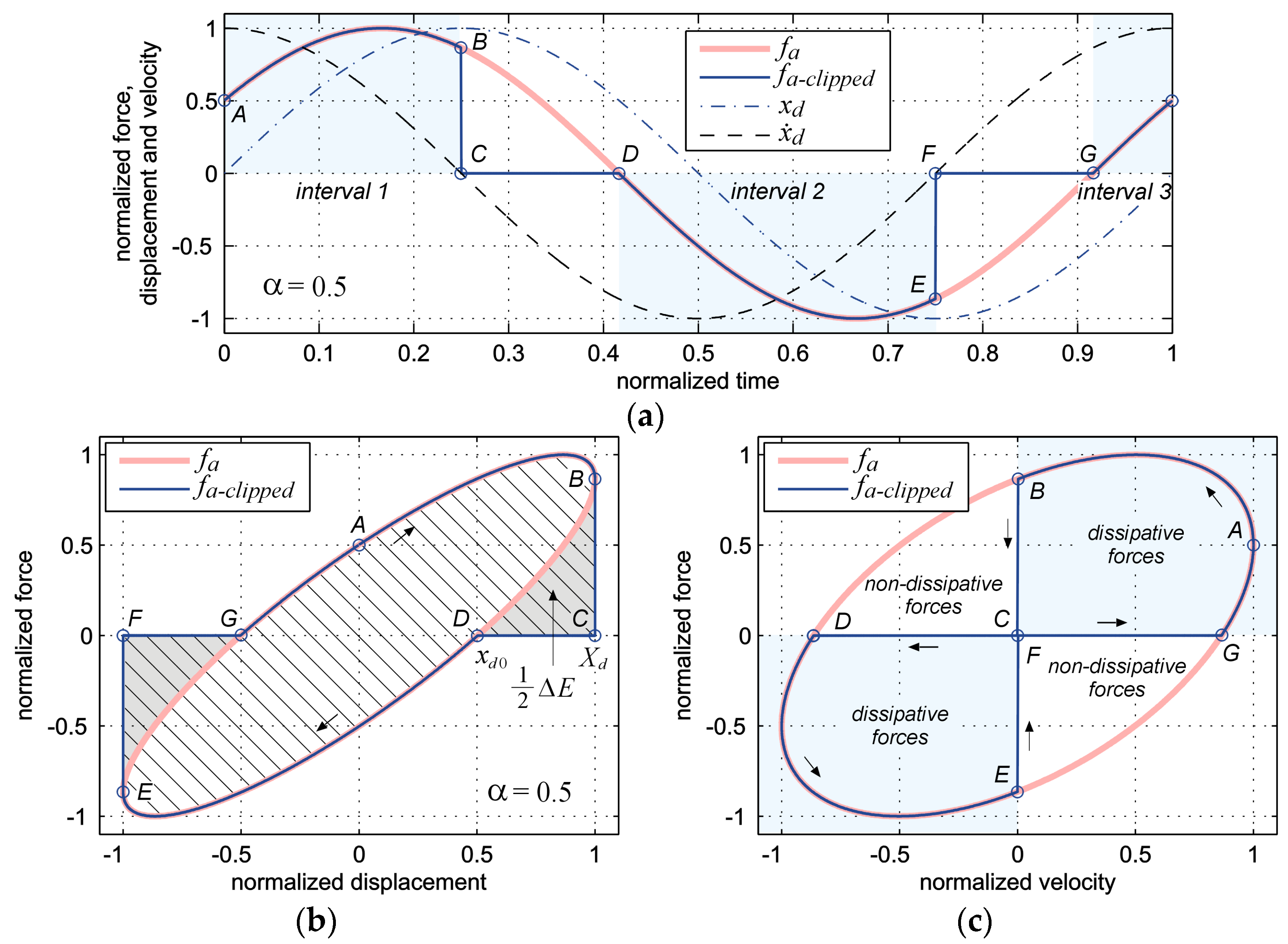
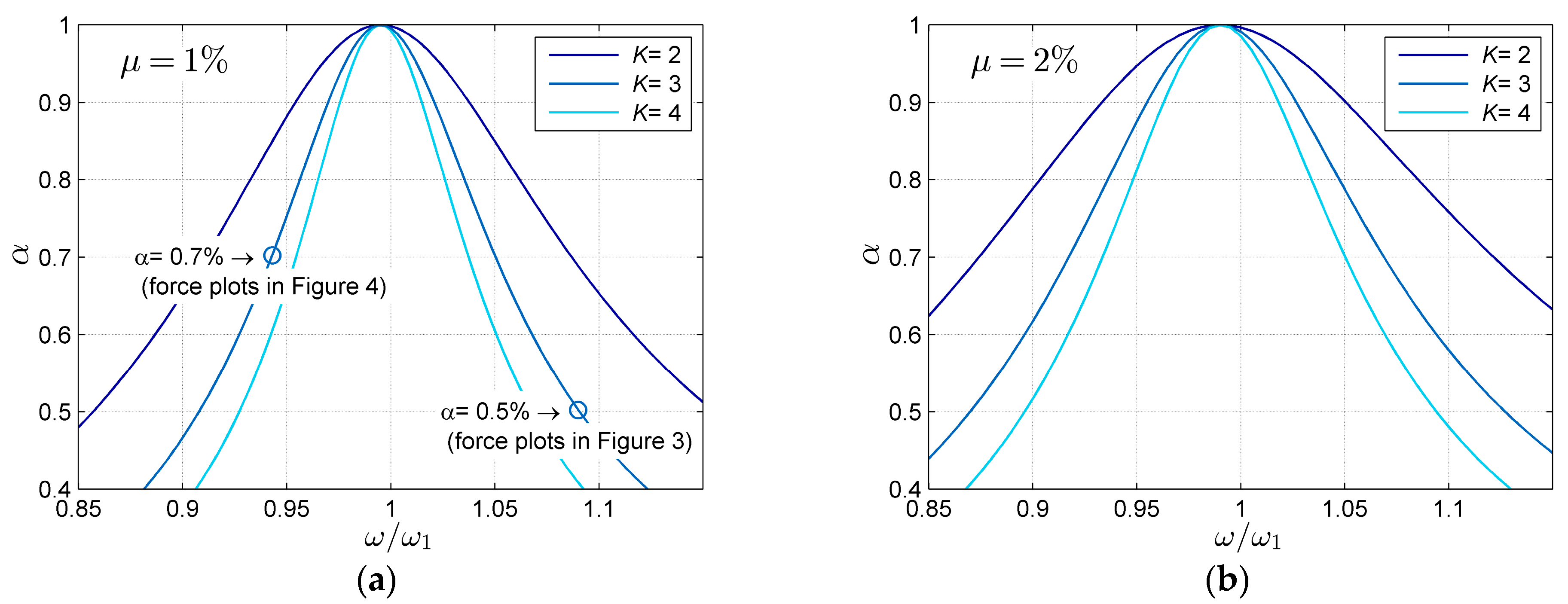
4.2. Examples of Force Characteristics

Figure 3 and Figure 4 show example characteristics of the control force f a and its clipped form f a c l i p p e d (33) as functions of time, relative displacement, and relative velocity.
The force characteristics in Figure 3 are presented for the case of positive stiffness k a , under conditions of moderate clipping. Figure 4 presents these characteristics for the case of negative stiffness k a , for a relatively small degree of clipping. Capital letters are used to label characteristic points in the figures to facilitate tracing the effect of force clipping simultaneously in terms of time, displacement, and velocity.
In Figure 3a and Figure 4a, the time intervals are marked where the force f a satisfies the condition f a x ˙ d > 0 , indicating that it has a dissipative character and can therefore be realized by a semi-active damper. The width of these intervals is not constant and depends on the frequency of vibrations ω as well as the parameters k a and c a .
For k a > 0 , the clipping necessitates an abrupt reduction of the semi-active damper force to zero whenever the sign of the relative velocity changes (points C and F in Figure 3). The clipping is then maintained until the control force f a , whose absolute value is decreasing, crosses zero (points D and G).
In the case of k a < 0 , the clipping occurs from the moment the control force f a crosses zero (points J and M, Figure 4) and initially does not require abrupt change of the force. However, resuming operation of the semi-active damper requires a sudden change in force from zero to the instantaneous value of f a (points K and N). More about the clipped viscous damping with negative stiffness can be found in [46,47].
The clipping operation represents a significant constraint and, if the active control force f a in (33) is optimal, then the clipped force (33) is no longer optimal. However, it is not obvious how exactly the clipping affects the resulting stiffness and damping, depending on the degree of clipping. This issue will be addressed below.

4.3. Description of Force Clipping Degree Using the Clipping Coefficient

A description of the clipping should begin with the introduction of a clipping coefficient, which will allow for an assessment of how much the clipped force differs from the unclipped force. For the purposes of this work, the clipping coefficient will be introduced based on the analysis of the force as a function of displacement.
Figure 3b and Figure 4b show an ellipse representing the force f a as a function of the relative displacement x d . For k a > 0 , this ellipse can be described by:
f e 1 = c a ω X d 2 x d 2 + k a x d ,
f e 2 = c a ω X d 2 x d 2 + k a x d ,
where f e 1 and f e 2 denote the parametric representation of the higher and lower branches of the ellipse, respectively.
The positive root of f e 2 , that is, the positive displacement at which the force f e 2 becomes zero (see point D in Figure 3b) is:
x d 0 = X d c a ω k a 2 + c a 2 ω 2 .
Based on (36), the clipping coefficient α is introduced as follows:
α = x d 0 X d = c a ω k a 2 + c a 2 ω 2 .
The clipping coefficient ranges from 1 (no clipping, the case of pure viscous damping, k a = 0 ), through a middle value of 0.5 (moderate clipping, for k a = 3 c a ω ), to 0 (maximal clipping, for c a = 0 ).
Figure 5 presents α as a function of normalized frequency for the sub-optimal STMD with mass ratio μ of 1% and 2%, for three selected values of K. Due to their presentation in terms of normalized frequency, the plots are independent of the structural parameters ( m 1 , ω 1 ). They depend solely on μ and K , which determine the values of k a and c a . The degree of clipping, described by α , is also independent of the forcing amplitude. Figure 5 indicates small and moderate degree of clipping for the sub-optimal STMD for typical values of μ and K in the considered frequency range. In Figure 5a, the two values of α are marked, corresponding to the cases of force characteristics in Figure 3 and Figure 4.

4.4. Energy Dissipation Resulting from Clipping

Another aspect in the analysis of the clipping operation concerns its impact on the energy dissipation during a vibration cycle. As illustrated by the force-displacement loops in Figure 3b and Figure 4b, the clipping augments cycle energy dissipation. This is evident from the enlargement of the area enclosed by the force-displacement plot. This area is quantitatively equal to the cycle energy.
The total cycle energy resulting from the clipped force (33) is represented by the dashed area in Figure 3b and can be expressed as:
E c l i p p e d = E u n c l i p p e d + Δ E ,
where E u n c l i p p e d = π ω c a X d 2 is the cycle energy due to the active control force f a , and Δ E denotes the increase in cycle energy due to the clipping. This additional energy Δ E is represented by the shaded areas in Figure 3b and, for k a > 0 , can be calculated as:
Δ E = 2 x d 0 X d f e 2 d x d .
where f e 2 and x d 0 are given by (35) and (36), respectively.
Evaluating the integral in (39) yields an analytical expression for the increase in cycle energy due to the clipping that is valid for both positive and negative stiffness k a :
Δ E = X d 2 ( c a ω ( α 1 α 2 + arcsin ( α ) π 2 ) | k a | ( α 2 1 ) ) .
After substituting (40) into (38), the total cycle energy resulting from the clipped force (33) is expressed as ((40) with the sign before the π / 2 term changed):
E c l i p p e d = X d 2 ( c a ω ( α 1 α 2 + arcsin ( α ) + π 2 ) | k a | ( α 2 1 ) ) .
The above expression can be employed to derive the energy-equivalent viscous damping coefficient, c e q , by equalizing   E c l i p p e d = π ω c e q X d 2 . However, to establish a full equivalent model for the clipped force (33), an adequate equivalent linearization method must be employed to also derive an equivalent stiffness.

4.5. Calculation of Equivalent Viscous Damping and Equivalent Stiffness for the Clipped Viscous Damping–Stiffness Force Using Harmonic Balance Method

The method of equivalent linearization by Krylov and Bogoliubov [48] is a well-established analytical technique based on the harmonic balance method for linearizing non-linear systems. It can be used to replace a non-linear function of strongly non-linear systems, see e.g., [49], with an equivalent linear function. In the context of semi-active vibration control systems, a good example can be found in [50].
Using this method, the equivalent damping and stiffness are determined by multiplying the force (33) by cos ( ω t ) and sin ( ω t ) , respectively, and then integrating the resulting expressions over a full vibration period:
c e q = 1 X d π 0 2 π / ω f a c l i p p e d cos ( ω t ) d t ,
k e q = ω X d π 0 2 π / ω f a c l i p p e d sin ( ω t ) d t .
Detailed analytical calculations for integrals (42) and (43) are provided in Appendix B. As an outcome of these calculations, the following expressions are derived:
c e q = c a 2 + c a arcsin ( α ) π + c a sin ( 2 arcsin ( α ) ) 2 π | k a | ( α 2 1 ) π ω ,
k e q = k a 2 + k a arcsin ( α ) π k a sin ( 2 arcsin ( α ) ) 2 π sgn ( k a ) c a ω ( α 2 1 ) π .
It should be noted that although the amplitude of relative motion X d appears in (42) and (43), the resulting equivalent model is independent of the amplitude X d . Consequently, the equivalent model is independent of the amplitude of force excitation. This feature holds true only for harmonic motion. The equivalent model, represented by equations (44) and (45), will be used later to analyze the frequency responses of the STMD.
In Figure 6, sample calculations of the equivalent viscous damping and the equivalent stiffness are presented for the sub-optimal STMD with μ = 1 % and K = 3. The calculations were conducted using the sample parameters listed in Section 3.5.
The greater the difference between ω and ω 1 , the more the degree of clipping increases. Consequently, both the amount of additional energy dissipated and the resulting equivalent viscous damping coefficient c e q rise. As an effect, c e q significantly exceeds c a (Figure 6a). In the case of stiffness (Figure 6b), the resulting equivalent stiffness, k e q , is noticeably smaller in magnitude than k a . Furthermore, the difference between k a and k e q becomes larger as the difference between ω and ω 1 increases.
The cumulative impact of clipping on both damping and stiffness adversely affects the performance of the sub-optimal STMD, as will be demonstrated in the following.

4.6. Numerical Analysis of Sub-Optimal STMD

Figure 7 presents the frequency responses calculated for the sub-optimal STMD with μ = 1%, for six different values of K from 2 to 20, in comparison to the frequency responses obtained for the TMD. These results clearly indicate that the performance of the sub-optimal STMD is noticeably worse than that of the ATMD (Figure 2). This is attributed to the described increase in damping and reduction in stiffness as the result of clipping.
For normalized frequencies ω / ω 1 close to 1, the control force (33) is minimally affected by clipping. As a result, in this frequency range, the sub-optimal STMD operates as intended, and the resulting vibration amplitude X 1 is consistent with that for the TMD with an enlarged mass ratio K μ (Figure 7a). Specifically, when ω = ω 1 / μ + 1 , the stiffness k a becomes zero, making the control force of the STMD purely dissipative. At this central frequency, the performance of the STMD is equivalent to that of the ATMD.
The numerical analysis revealed that the sub-optimal STMD has a clear limit in effectiveness, determined as the smallest achievable value of maximum dynamic amplification factor ( D A F m a x ). For μ = 1 % , the calculations show that the minimum D A F m a x of 10.27 is achieved for K = 4.04 , as indicated by the red line in Figure 7a. Increasing K beyond 4.04 can only result in an increase in D A F m a x , with a slightly higher right peak.
Additional significant limitations of the sub-optimal STMD are evident in Figure 7b. The maximum relative displacement for the sub-optimal STMD far exceeds that of a TMD with the same mass. Such performance from STMD is considered unacceptable. In practice, constraining the relative motion is crucial due to spatial limitations at the installation site of the mass damper. Active and semi-active solutions are expected to fit within the same space as a TMD with the same mass. This consideration is also taken into account in the subsequent numerical optimization of the STMD.
Note that the frequency responses shown in Figure 7 were calculated using (16) and (17), as previously in Section 3.5. However, in these calculations, c a and k a were substituted with the equivalent model c e q (44) and k e q (45), respectively. To assess the accuracy of the equivalent model, analogous steady-state frequency responses were also determined through simulations in MATLAB/Simulink. Based on this comparison, it was determined that regardless of the amplitude of force excitation, the maximum discrepancy between the calculated and simulated amplitude X 1 in the steady state does not exceed 0.58% for K = 3, 0.93% for K = 4, and 2.7% for K = 20. Therefore, the equivalent model (44) and (45) is assumed to be sufficiently accurate and useful in predicting the frequency responses of the primary structure equipped with the STMD.
Appendix A provides the MATLAB code for calculating the frequency responses for the sub-optimal STMD.

5. Calibration of STMD Using Numerical Optimization

The control force of the sub-optimal STMD, as previously discussed, lacks adjustments to mitigate the effects of force clipping. In this section, an optimized STMD featuring necessary modifications to its control force is presented. These modifications are aimed at compensating for the effects of clipping to the extent possible, thereby improving the calibration and overall performance of the STMD.
A modified semi-active control force with two incorporated correction factors is subsequently introduced, designed to scale the control force before clipping occurs. The numerical optimization procedure used to calibrate these correction factors are then outlined. Finally, the optimization results as well as an analysis of the optimized STMD at its performance limit are presented.

5.1. Semi-Active Control Force

The semi-active control force f s a for the STMD depicted in Figure 1c is defined as:
f s a = { c s a x ˙ d + k s a x d : ( c s a x ˙ d + k s a x d ) x ˙ d > 0 0 : o t h e r w i s e ,
where c s a and k s a are the modified force parameters, formulated similarly as before, see (31) and (32), but incorporating correction factors K c o r and c c o r :
c s a = c c o r m 1 ω 1 3 μ 3 2 K c o r K ( 1 + μ ) 3 ,
k s a = m 1 K c o r K μ μ K c o r K μ + K c o r K ( ω 2 ω 1 2 μ + 1 ) .
The adoption of the modified control force in the form (46) is based on an analysis of the operation of the sub-optimal STMD. The introduction of K c o r is necessary to achieve the proper effectiveness, which is defined for the design parameter K in the same manner as for the ATMD (see (13)). The parameter c c o r allows for adjustment of damping, which will enable control of the frequency response of the STMD around the central frequency between the two peaks.
It should be noted that the introduction of the correction factors in the notations of relative velocity and displacement feedback gains for the control force of STMD was previously presented in [42]. The method used in [42] is very similar; however, it was applied to a differently defined control force with an additional feedback loop from acceleration.

5.2. Objective and Procedure of Optimization

In the case of the sub-optimal STMD, a clear performance limit was observed and manifested as the smallest achievable value of D A F m a x (Figure 7a). Therefore, the first natural objective of optimizing the STMD was to determine the best calibration of the STMD force parameters for the highest possible efficiency, exceeding that of the sub-optimal STMD.
The main objective of optimization was to determine the STMD force parameters for various K and μ , in such a way as to minimize the differences in efficiency between the STMD and the ATMD for a given K . It was also assumed that the optimized STMD must satisfy the condition concerning the amplitude of relative displacement X d , which cannot exceed that for a TMD with the same mass and for the same excitation.
The numerical optimization was carried out in MATLAB using the unconstrained minimization method implemented as the fminsearch function. The objective function J ( v ) to be minimized using the fminsearch function was defined based on the dynamic amplification of the primary structure displacement, as introduced in [42]. This objective function consists of the sum of squared differences between the local peaks, and the local minimum between those peaks, for both the STMD with specific μ and K , and the Den Hartog’s TMD with mass ratio K μ :
J ( v ) = ( P s a ( v ) P ) 2 + ( Q s a ( v ) Q ) 2 + ( S s a ( v ) S ) 2 ,
where v = [ K c o r   c c o r ] is a vector of the optimization variables; P s a ( v ) , Q s a ( v ) and S s a ( v ) are, respectively, the left and right local peaks and the local minimum in between those peaks of the frequency response X 1 / X 1 s t a t i c of the primary structure with the STMD of mass ratio μ and control parameter K; while P, Q and S are the corresponding quantities for the TMD with mass ratio K μ .
Specifically, the objective function (49) assumes a zero value when the two peaks of the frequency response for the STMD are equal and match the value given by (13), and when the local minimum is as for the TMD with mass ratio of K μ .
The fminsearch function was run with an initial estimate of the optimization variables v = [1 1]. The maximum number of iterations allowed was set to 400. In each iteration of the optimization, the actual feedback gains c s a (47), k s a (48) and the corresponding equivalent model c e q (44), k e q (45) are calculated for the current estimate of optimization variables K c o r ,   c c o r . Then, the frequency response of the primary structure with the STMD is determined, as well as the current value of the objective function (49). The frequency responses are calculated using (16), but with c e q and k e q instead of c a and k a . This approach allows for rapid frequency response calculations in each iteration, leading to quickly obtained optimization results even for large number of iterations.
The optimization was conducted for the sample model parameters listed in Section 3.5, for various K , and for μ ranging from 0.4% to 3%.

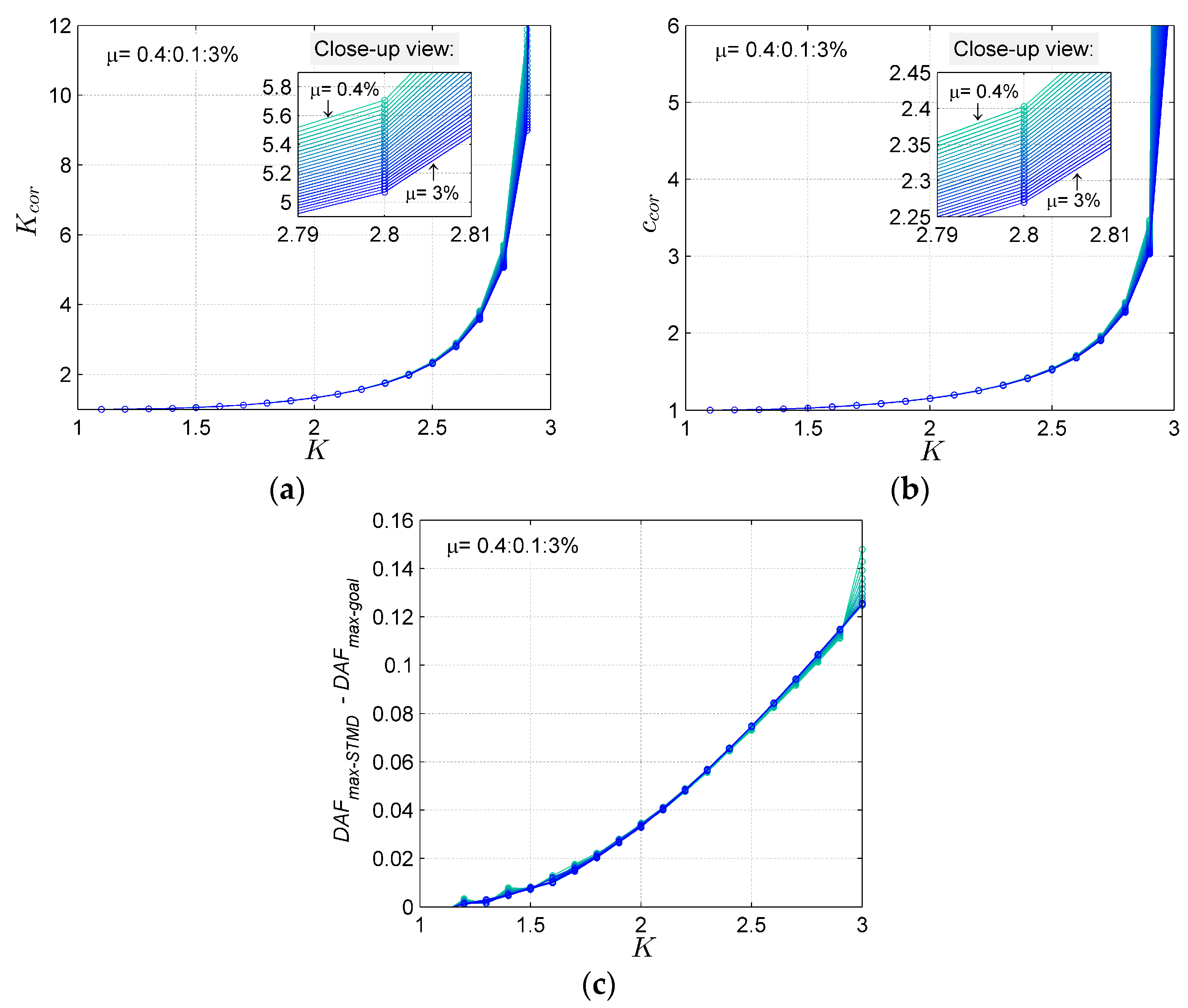
5.3. Optimization Results

An important observation from the optimization is that the optimized STMD reaches a clear efficiency limit around K = 3 . For K > 3 , the optimization yields disproportionately large values of K c o r and c c o r without achieving further improvement in the STMD efficiency.
The optimized correction factors K c o r and c c o r are plotted in Figure 8a,b versus K from 1 to 3 and for various μ from 0.4% to 3%. Within the range of values presented in these figures, both K c o r and c c o r increase with K in a similar manner for each mass ratio μ .
Figure 8c shows the difference between the maximum DAF (10) values calculated for the optimized STMD with mass ratio μ and the reference TMD with mass ratio K μ . This difference serves as a straightforward measure for assessing the results of optimization. The maximum value in Figure 8c is 0.148, obtained for K = 3 and μ = 0.4 % . This value implies that the peak response of the STMD exceeds the target D A F m a x = 12.95 by 1.14%. Similarly, when K = 3 and μ = 3 % , the maximum difference is 0.125, indicating that the STMD’s peak response is 2.6% above the targeted value of 4.82. Given that the maximum percentage error is under 3%, the optimization outcomes are considered acceptable.
Table 1 lists the optimized values of K c o r and c c o r for selected K ranging from 1.5 to 3, and for three typical μ of 0.5%, 1%, and 2%. It is noticeable that the values for K = 3 are exceptionally high compared to the rest of the results. When K is slightly reduced to 2.98, these values become significantly smaller. This is because, for K = 3, the optimized STMD is already at its performance limit.

5.4. Analysis of the Optimized STMD at Its Performance Limit

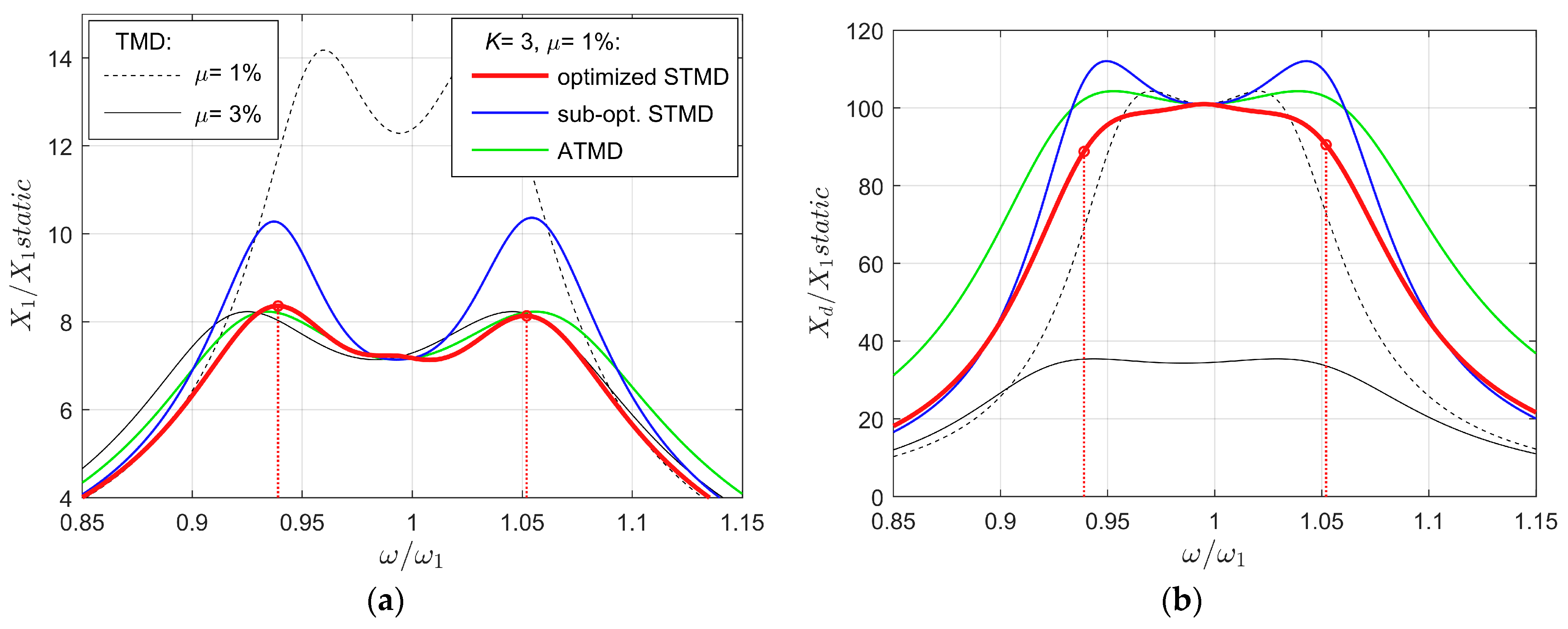
5.4.1. Frequency Responses

Figure 9 presents the frequency responses for the optimized STMD with mass ratio μ = 1 % and the highest achievable efficiency at K = 3 . The results for the optimized STMD are compared with those for the sub-optimal STMD and the ATMD (both with the same μ and K ). For additional context, this figure also includes results for the TMD with μ = 1% and 3%.
Figure 9a confirms that the optimized STMD performs significantly better than the sub-optimal STMD and nearly as well as the ATMD with the same K . More precisely, while the shapes of the responses for the STMD and ATMD are slightly different, the left peak of the STMD response is 2.4% higher and the right peak is slightly smaller than that of the ATMD.
Significantly, the maximum amplitude of relative displacement for the optimized STMD is not greater than that for the TMD and ATMD with the same mass ratio. In fact, the relative displacement for the optimized STMD is lower than that for the ATMD across the entire frequency range, as shown in Figure 9b.

5.4.2. Characterization of the Control Force

It is underlined that the enhanced efficiency of the optimized STMD is not associated with extensive control force demands. In Figure 10a, the force demands for the semi-active damper in the STMD are compared with those for the active actuator in the ATMD and the viscous damper in the TMDs. The figure displays the maximum force requirements at steady-state as a function of frequency, assuming a force excitation of F e x c = 8 kN.
Figure 10a reveals that the maximum control force of the optimized STMD is only 6% greater than that of the ATMD and 9% greater than that of the sub-optimal STMD. This occurs even though the optimized STMD at K = 3 is operating at its performance limit and the correction factors are significantly high. The only slight increase observed in the control force of the optimized STMD can be attributed to its dependency on relative motion, which is considerably reduced compared to both the sub-optimal STMD and ATMD, as previously explained. Note that the results in Figure 10a are not normalized. The actual force demands will depend on the assumed worst-case excitation force and the specific model parameters.
Figure 10b provides further insights into the control force characteristics of the optimized STMD by comparing the clipping coefficients α for both the optimized and sub-optimal STMDs. Throughout the entire frequency range, the degree of force clipping for the optimized STMD is noticeably higher ( α is smaller) than for the sub-optimal STMD. This difference arises because the optimized stiffness k s a used in the calculations of the control force (46) is significantly greater than its corresponding value k a in the sub-optimal STMD. The active force component, k s a x d , consequently intensifies, leading to a higher degree of clipping. In the following, we discuss how this increased stiffness force enhances the efficiency of the optimized STMD, despite the higher degree of force clipping.

5.4.3. Analysis of the Force–Displacement Characteristics at Crucial Frequencies

Figure 11a,b provide a comparison of the force–displacement characteristics between the optimized STMD and the sub-optimal STMD at two specific frequencies. These frequencies correspond to the left and right peaks of the STMD response, as indicated by the red dotted lines in Figure 9 and Figure 10.
The force plots in Figure 11 are supplemented with values for relevant parameters: k a (the optimal controlled stiffness of the ATMD, also used in force calculation for the sub-optimal STMD), k e q (the resultant equivalent stiffness after force clipping achieved for the sub-optimal STMD), k s a (the stiffness used in force calculation for the optimized STMD), and k e q o p t (introduced here to denote the equivalent stiffness resulting from the semi-active force of the optimized STMD, calculated using (45) but for k s a and c s a ). These parameters clearly demonstrate that the resultant equivalent stiffness k e q o p t for the optimized STMD is approximately equal to the optimal stiffness k a of the ATMD, for both positive and negative stiffness k a .
For a better illustration of this effect, Figure 11a,b include plots of the linear stiffness force k a x d of the optimal ATMD, as well as the equivalent linear stiffness forces k e q x d and k e q o p t x d for both the sub-optimal and the optimized STMD, respectively. Additionally, a comparison of the optimal stiffness k a , with the resulting equivalent stiffnesses k e q and k e q o p t , is presented as a function of frequency in Figure 11c. Based on these results, it can be concluded that the presented calibration method for the STMD enables precise control of both positive and negative stiffness. Around crucial frequencies of both peaks, the resulting equivalent stiffness for the optimized STMD is closely aligned with the optimal stiffness of the reference ATMD with the same mass ratio and K parameter. However, it should be emphasized that as the value of K increases, the absolute value of the optimal stiffness k a also increases (at a given frequency), while the demanded viscous damping c a decreases. According to the previous analysis, increasing k a leads to a higher degree of clipping. This, in turn, results in greater cycle energy dissipation, as well as increased the resultant equivalent viscous damping. As a result, it is not possible to satisfy both the demands for increased stiffness and decreased damping simultaneously. This leads to an inherent performance limit of the STMD.

6. Conclusions

This paper investigated both active and semi-active tuned mass dampers with relative displacement and velocity feedback. Following the approach in [42], both mass dampers were calibrated for the specific parameter K, ensuring that their effectiveness in reducing harmonic vibrations is comparable to that of the Den Hartog’s TMD with K times larger mass. The key conclusions drawn from this work are as follows:
  • The optimal ATMD with acceleration feedback proposed by Nishimura et al. [17] can alternatively be realized based on a relative displacement and velocity feedback, without relying on acceleration feedback.
  • Both the sub-optimal STMD and the optimized STMD with the clipped viscous damping–stiffness control force have a clearly defined efficiency limit.
  • The application of the numerically optimized correction factors in the semi-active control force (46)–(48) allowed us to achieve an enhanced performance of the optimized STMD compared to the sub-optimal STMD.
  • The highest effectiveness of the optimized STMD in reducing harmonic vibrations corresponds to the TMD with roughly three times greater mass.
Although the results presented in this work are promising, they should be treated as primarily theoretical due to the assumptions made regarding the use of an ideal semi-active damper in the STMD and an ideal active actuator in the ATMD. In practice, the effectiveness of both systems will be limited, in part, due to the force tracking errors, which are discrepancies between the ideal control force and its actual value. These aspects require further investigation in future research.

Funding

This research was funded by the AGH University of Krakow within the scope of the Research Program No. 16.16.130.942.

Institutional Review Board Statement

Not applicable.

Informed Consent Statement

Not applicable.

Data Availability Statement

Data are contained within the article.

Conflicts of Interest

The author declares no conflict of interest.

Appendix A. MATLAB Code

For the reader’s convenience, the MATLAB code comparing the frequency responses for the ATMD, sub-optimal STMD, optimized STMD, and TMD is provided. The main script, responsible for calculating and plotting the responses, can be found in Table A1. This script utilizes the following functions:
  • ‘mm_FRF.m’ (Table A2): Calculates the frequency response;
  • ‘mm_fa_gains.m’ (Table A3) and ‘mm_fsa_gains.m’ (Table A4): Compute the parameters for active and semi-active control forces, respectively;
  • ‘mm_DH_tuning.m’ (Table A5): Implements the Den Hartog tuning;
  • ‘mm_equiv_linear.m’ (Table A6): Performs the equivalent linearization of the clipped viscous damping–stiffness force.
For each formula implemented in the code, the corresponding equation number from the paper is provided.
Table A1. MATLAB script comparing the frequency responses for the ATMD, STMD, and TMD.
% Paper_demo.m
% Calculations and plots of the frequency responses for the ATMD, STMD, and TMD
close all, clear all
%% Design parameters (adjust, see Table 1 for Kcor and ccor)
K = 3; mu = 1/100; Kcor = 890.90; ccor = 30.165;
% K = 2.8; mu =1/100; Kcor = 5.5289; ccor = 2.3679;
% K = 2.6; mu = 1/100; Kcor = 2.8751; ccor = 1.7019;
% K = 2; mu = 1/100; Kcor = 1.3331; ccor = 1.1539;
%% Model parameters
f1 = 0.5; % natural frequency, Hz
om1 = 2*pi*f1; % natural frequency, rad/s
m1 = 500e3; % structure mass, kg
Fexc = 8e3; % amplitude of force excitation, N
k1 = om1^2*m1; % structure stiffness, N/m
m2 = m1*mu; % mass, kg
om = om1*[0.7:2e-3:1.3]; % frequency of excitation vector, rad/s
%% TMDs design and frequency responses for mass ratio mu and K*mu
[k2dh, c2dh] = mm_DH_tuning(m1, om1, mu);
[k2dhK,c2dhK] = mm_DH_tuning(m1, om1, K*mu);
[TMD1_DAFX1,TMD1_DAFXd] = mm_FRF(m1, om1, m2, k2dh, c2dh, om, Fexc);
[TMD2_DAFX1,TMD2_DAFXd] = mm_FRF(m1, om1, K*m2, k2dhK, c2dhK, om, Fexc);
%% ATMD design and frequency responses for mass ratio mu
[ca, ka] = mm_fa_gains(K, m1, om1, mu, om);
[ATMD_DAFX1, ATMD_DAFXd] = mm_FRF(m1, om1, m2, (k2dh+ka), ca, om, Fexc);
%% Sub-optimal STMD - frequency responses for mass ratio mu
[keq, ceq, alpha] = mm_equiv_linear(ka, ca, om);
[STMD_DAFX1sub,STMD_DAFXdsub]=mm_FRF(m1,om1,m2,(k2dh+keq),ceq,om,Fexc);
%% Optimized STMD design and frequency responses for mass ratio mu
[csa, ksa] = mm_fsa_gains(K, m1, om1, mu, om, Kcor, ccor);
[keqopt, ceqopt, alphaopt] = mm_equiv_linear(ksa, csa, om);
[STMD_DAFX1,STMD_DAFXd]=mm_FRF(m1,om1,m2,(k2dh+keqopt),ceqopt,om,Fexc);
%% Plots
figure
plot(om/om1, TMD1_DAFXd,‘--k’), hold on
plot(om/om1, TMD2_DAFXd,‘k’)
plot(om/om1, ATMD_DAFXd,‘g’)
plot(om/om1, STMD_DAFXdsub,‘b’)
plot(om/om1, STMD_DAFXd,‘r’)
xlabel(‘omega/omega1’), ylabel(‘Xd/X1static’), xlim([0.7 1.3])
figure
plot(om/om1, TMD1_DAFX1,‘--k’), hold on
plot(om/om1, TMD2_DAFX1,‘k’)
plot(om/om1, ATMD_DAFX1,‘g’)
plot(om/om1, STMD_DAFX1sub,‘b’)
plot(om/om1, STMD_DAFX1,‘r’)
xlabel(‘omega/omega1’), ylabel(‘X1/X1static’), xlim([0.7 1.3])
legend([‘TMD,\mu=’,num2str(100*mu),‘%’],[‘TMD,\mu=’,num2str(100*K*mu),‘%’],…
[‘ATMD,\mu=’,num2str(100*mu),‘%,K=’,num2str(K)],…
[‘STMD-sub,\mu=’,num2str(100*mu),‘%,K=’,num2str(K)],…
[‘STMD-opt,\mu=’,num2str(100*mu),‘%,K=’,num2str(K)])
Table A2. MATLAB function for the frequency response calculation.
function [DAFX1, DAFXd] = mm_FRF(m1, om1, m2, k2, c2, om, Fexc)
% Frequency response
% Outputs: DAFX1, DAFXd - dynamic amplifications of disp. amplitudes X1 and Xd
k1 = om1^2*m1; % structure’ stiffness, N/m
% Complex amplitudes of harmonic response:
num = k2-om.^2*m2 + 1i*om.*c2;
den = (k1-om.^2*(m1 + m2)).*(k2-om.^2*m2 + 1i*om.*c2) - om.^4*m2^2;
x1 = Fexc * num./den; % structural mass complex amplitude, Equation (8)
xd = Fexc * om.^2*m2 ./den; % relative complex amplitude, Equation (9)
% Displacement amplitudes:
X1 = abs(x1); % absolute amplitude X1 of mass m1, m
Xd = abs(xd); % relative amplitude Xd, m
% Dynamic amplification factors:
X1static = Fexc/k1; % static deflection due to the excitation force, m
DAFX1 = X1/X1static; % dynamic amplification of X1, Equation (10)
DAFXd = Xd/X1static; % dynamic amplification of Xd
Table A3. MATLAB function for calculation of the control force parameters of ATMD.
function [ca, ka] = mm_fa_gains(K, m1, om1, mu, om)
% Viscous damping–stiffness force parameters
% Outputs: ca, ka - parameters of the control force given by Equation (12)
ca = m1*om1*sqrt(3*mu^3/(2*K*(1 + mu)^3)); % Equation (31)
ka = m1* (K*mu-mu)/(K*mu + K) * (om.^2 - om1^2/(mu + 1)); % Equation (32)
Table A4. MATLAB function for calculation of the control force parameters of STMD.
function [csa, ksa] = mm_fsa_gains(K, m1, om1, mu, om, Kcor, ccor)
% Clipped viscous damping–stiffness force parameters
% Outputs: csa, ksa - parameters of the control force given by Equation (46)
csa = ccor*m1*om1*sqrt(3*mu^3/(2*K*Kcor*(1 + mu)^3));% Equation (47)
ksa = m1*(K*Kcor*mu-mu)/(K*Kcor*mu + K*Kcor)*(om.^2-om1^2/(mu + 1));% Equation (48)
Table A5. MATLAB function for calculation of the TMD parameters.
function [k2dh, c2dh] = mm_DH_tuning(m1, om1, mu)
% Den Hartog tuning, Equations (1) and (3)
% Outputs: k2dh - stiffness, N/m; c2dh - viscous damping, Ns/m
m2 = mu*m1; % mass, kg
om2 = om1/(1 + mu); % frequency, rad/s
k2dh = om2^2*m2; % spring stiffness, N/m
dzeta2 = sqrt(3/8*mu/(1 + mu)); % damping ratio
c2dh = 2*dzeta2*m2*om2; % viscous damping coefficient, Ns/m
Table A6. MATLAB function for the equivalent linearization of the clipped control force.
function [keq, ceq, alpha] = mm_equiv_linear(ka, ca, om)
% Equivalent linearization of the clipped viscous damping–stiffness control force
% Outputs: keq, ceq - equivalent stiffness and equivalent viscous damping,
% alpha - clipping coefficient
alpha = ca.*om ./sqrt(ka.^2 + om.^2.*ca.^2);% Equation (37)
ceq = ca/2 + ca.*asin(alpha)/pi + ca.*sin(2*asin(alpha))/(2*pi) -…
sign(ka).*ka.*(alpha.^2 -1)./(pi*om); % Equation (44)
keq = ka/2 - sign(ka).*ca.*om.*(alpha.^2 -1)/pi + ka.*asin(alpha)/pi -…
ka.*sin(2*asin(alpha) )/(2*pi); % Equation (45)

Appendix B. Analytical Calculations of Integrals in the Equivalent Linearization for a Clipped Viscous Damping–Stiffness Force

We calculate the integrals in (42) and (43) as the sum of the definite integrals in those time intervals where the force is not clipped to zero. For harmonic displacement x d = X d sin ( ω t ) , and velocity x ˙ d = ω X d cos ( ω t ) ,   (42) and (43) can be expressed as:
c e q = 1 X d π 0 2 π / ω ( c a ω X d cos ( ω t ) + k a X d sin ( ω t ) ) cos ( ω t ) d t ,
k e q = ω X d π 0 2 π / ω ( c a ω X d cos ( ω t ) + k a X d sin ( ω t ) ) sin ( ω t ) d t .
To facilitate the description, let us assume:
k e q = A + B ,
c e q = C + D ,
where for the harmonic motion, the integrals A, B, C, D become independent of the amplitude X d :
A = c a ω 2 π 0 2 π / ω sin ( ω t ) cos ( ω t ) d t ,
B = k a ω π 0 2 π / ω sin 2 ( ω t ) d t ,
C = c a ω π 0 2 π / ω cos 2 ( ω t ) d t ,
D = k a π 0 2 π / ω sin ( ω t ) cos ( ω t ) d t .
Integrals (A5)–(A8) will be calculated in the three intervals marked in Figure 4a, for the case of negative stiffness k a . The interval 1 is defined from 0 to the time instant corresponding to point J in Figure 4a and can be given by (0, arcsin ( α ) / ω ), where α is the clipping coefficient (37). Integration over the time interval 1 yields:
A 1 = c a ω 2 π 0 arcsin ( α ) / ω sin ( ω t ) cos ( ω t ) d t = α 2 c a ω 2 π ,
B 1 = k a ω π 0 arcsin ( α ) ω sin 2 ( ω t ) d t = k a arcsin ( α ) 2 π k a sin ( 2 arcsin ( α ) ) 4 π ,
C 1 = c a ω π 0 arcsin ( α ) ω cos 2 ( ω t ) d t = c a arcsin ( α ) 2 π + c a sin ( 2 arcsin ( α ) ) 4 π ,
D 1 = k a π 0 arcsin ( α ) ω sin ( ω t ) cos ( ω t ) d t = α 2 k a 2 π ω .
The interval 2, from point K to M in Figure 4a, is given by ( π 2 ω , π + arcsin ( α ) ω ). By calculating the integrals within this interval, we obtain:
A 2 = c a ω 2 π π 2 ω π + arcsin ( α ) ω sin ( ω t ) cos ( ω t ) d t = c a ω ( α 2 1 ) 2 π ,
B 2 = k a ω π π 2 ω π + arcsin ( α ) ω sin 2 ( ω t ) d t = k a arcsin ( α ) 2 π k a sin ( 2 arcsin ( α ) ) 4 π + k a 4 ,
C 2 = c a ω π π 2 ω π + arcsin ( α ) ω cos 2 ( ω t ) d t = c a arcsin ( α ) 2 π + c a sin ( 2 arcsin ( α ) ) 4 π + c a 4 ,
D 2 = k a π π 2 ω π + arcsin ( α ) ω sin ( ω t ) cos ( ω t ) d t = ( α 2 1 ) k a 2 π ω .
Similarly, we compute the integrals in interval 3, which is defined in Figure 4a from point N to the end of the period. This interval is given by ( 3 π 2 ω , 2 π ω ). The integrals are:
A 3 = c a ω 2 π 3 π 2 ω 2 π ω sin ( ω t ) cos ( ω t ) d t = c a ω 2 π ,
B 3 = k a ω π 3 π 2 ω 2 π ω sin 2 ( ω t ) d t = k a 4 ,
C 3 = c a ω π 3 π 2 ω 2 π ω cos 2 ( ω t ) d t = c a 4 ,
D 3 = k a π 3 π 2 ω 2 π ω sin ( ω t ) cos ( ω t ) d t = k a 2 π ω .
The sums of the integrals in the respective intervals are:
A = A 1 + A 2 + A 3 = c a ω ( α 2 1 ) π ,
B = B 1 + B 2 + B 3 = k a arcsin ( α ) π k a sin ( 2 arcsin ( α ) ) 2 π + k a 2 ,
C = C 1 + C 2 + C 3 = c a arcsin ( α ) π + c a sin ( 2 arcsin ( α ) ) 2 π + c a 2 ,
D = D 1 + D 2 + D 3 = α 2 k a 2 π ω + ( α 2 1 ) k a 2 π ω k a 2 π ω .
Ultimately, for k a < 0 , we obtain:
c e q = C + D = c a 2 + c a arcsin ( α ) π + c a sin ( 2 arcsin ( α ) ) 2 π + k a ( α 2 1 ) π ω ,
k e q = A + B = k a 2 + k a arcsin ( α ) π k a sin ( 2 arcsin ( α ) ) 2 π + c a ω ( α 2 1 ) π .
After conducting the same calculations for k a > 0 , for the three intervals marked in Figure 3a, we can derive c e q and k e q in the same form but with an opposite sign for the last term in both (A25) and (A26). Considering this change of the sign allows us to present the final expressions, for both positive and negative k a , as follows:
c e q = c a 2 + c a arcsin ( α ) π + c a sin ( 2 arcsin ( α ) ) 2 π | k a | ( α 2 1 ) π ω ,
k e q = k a 2 + k a arcsin ( α ) π k a sin ( 2 arcsin ( α ) ) 2 π sgn ( k a ) c a ω ( α 2 1 ) π

References

  1. Elias, S.; Matsagar, V. Research developments in vibration control of structures using passive tuned mass dampers. Annu. Rev. Control 2017, 44, 129–156. [Google Scholar] [CrossRef]
  2. Koutsoloukas, L.; Nikitas, N.; Aristidou, P. Passive, semi-active, active and hybrid mass dampers: A literature review with associated applications on building-like structures. Dev. Built Environ. 2022, 12, 100094. [Google Scholar] [CrossRef]
  3. Fujino, Y.; Siringoringo, D. Vibration Mechanisms and Controls of Long-Span Bridges: A Review. Struct. Eng. Int. 2013, 23, 248–268. [Google Scholar] [CrossRef]
  4. Li, Q.S.; Zhi, L.H.; Tuan, A.Y.; Kao, C.S.; Su, S.C.; Wu, C.F. Dynamic behavior of Taipei 101 tower: Field measurement and numerical analysis. J. Struct. Eng. 2010, 137, 143–155. [Google Scholar] [CrossRef]
  5. Den Hartog, J.P. Mechanical Vibrations; McGraw-Hill: New York, NY, USA, 1956. [Google Scholar]
  6. Burton, M.D.; Kwok, K.C.S.; Abdelrazaq, A. Wind-induced motion of tall buildings: Designing for occupant comfort. Int. J. High-Rise Build. 2015, 4, 1–8. [Google Scholar]
  7. Hayes, J. Tall storeys. Eng. Technol. 2018, 13, 70–73. [Google Scholar] [CrossRef]
  8. Yao, J.T. Concept of structural control. J. Struct. Div. 1972, 98, 1567–1574. [Google Scholar] [CrossRef]
  9. Nishitani, A. Obituary for Professor Takuji Kobori: Great pioneer in structural dynamics and control. Struct. Control Health Monit. 2008, 15, 117–119. [Google Scholar] [CrossRef]
  10. Chang, J.C.H.; Soong, T.T. Structural control using active tuned mass dampers. J. Eng. Mech. Div. 1980, 106, 1091–1098. [Google Scholar] [CrossRef]
  11. Kobori, T.; Koshika, N.; Yamada, K.; Ikeda, Y. Seismic-response-controlled structure with active mass driver system. Part 1: Design. Earthq. Eng. Struct. Dyn. 1991, 20, 133–149. [Google Scholar] [CrossRef]
  12. Ikeda, Y. Active and semi-active vibration control of buildings in Japan—Practical applications and verification. Struct. Control Health Monit. 2009, 16, 703–723. [Google Scholar] [CrossRef]
  13. Spencer, B.F.; Nagarajaiah, S. State of the art of structural control. J. Struct. Eng. 2003, 129, 845–856. [Google Scholar] [CrossRef]
  14. Casciati, F.; Rodellar, J.; Yildirim, U. Active and semi-active control of structures—Theory and applications: A review of recent advances. J. Intell. Mater. Syst. Struct. 2012, 23, 1181–1195. [Google Scholar] [CrossRef]
  15. Zhou, K.; Zhang, J.W.; Li, Q.S. Control performance of active tuned mass damper for mitigating wind-induced vibrations of a 600-m-tall skyscraper. J. Build. Eng. 2021, 45, 103646. [Google Scholar] [CrossRef]
  16. Zhou, K.; Li, Q.S. Vibration mitigation performance of active tuned mass damper in a super high-rise building during multiple tropical storms. Eng. Struct. 2022, 269, 114840. [Google Scholar] [CrossRef]
  17. Nishimura, I.; Kobori, T.; Sakamoto, M.; Koshika, N.; Sasaki, K.; Ohrui, S. Active tuned mass damper. Smart Mater. Struct. 1992, 1, 306–311. [Google Scholar] [CrossRef]
  18. Asami, T.; Nishihara, O.; Baz, A.M. Analytical solutions to H and H2 optimization of dynamic vibration absorbers attached to damped linear systems. J. Vib. Acoust. 2002, 124, 284–295. [Google Scholar] [CrossRef]
  19. Deraemaeker, A.; Soltani, P. A short note on equal peak design for the pendulum tuned mass dampers. Proc. Inst. Mech. Eng. Part K J. Multi-Body Dyn. 2016, 231, 285–291. [Google Scholar] [CrossRef]
  20. Habib, G.; Detroux, T.; Viguié, R.; Kerschen, G. Nonlinear generalization of Den Hartog’s equal-peak method. Mech. Syst. Signal Process. 2015, 52, 17–28. [Google Scholar] [CrossRef]
  21. Chatterjee, S. Optimal active absorber with internal state feedback for controlling resonant and transient vibration. J. Sound Vib. 2010, 329, 5397–5414. [Google Scholar] [CrossRef]
  22. Cheung, Y.L.; Wong, W.O.; Cheng, L. Design optimization of a damped hybrid vibration absorber. J. Sound Vib. 2012, 331, 750–766. [Google Scholar] [CrossRef]
  23. Brodersen, M.L.; Bjørke, A.-S.; Høgsberg, J. Active tuned mass damper for damping of offshore wind turbine vibrations. Wind Energy 2017, 20, 783–796. [Google Scholar] [CrossRef]
  24. Koo, J.H.; Goncalves, F.D.; Ahmadian, M.A. Comprehensive analysis of the response time of MR dampers. Smart Mater. Struct. 2006, 15, 351–358. [Google Scholar] [CrossRef]
  25. Strecker, Z.; Roupec, J.; Mazurek, I.; Machacek, O.; Kubik, M.; Klapka, M. Design of magnetorheological damper with short time response. J. Intell. Mater. Syst. Struct. 2015, 26, 1951–1958. [Google Scholar] [CrossRef]
  26. Zhu, X.; Jing, X.; Cheng, L. Magnetorheological fluid dampers: A review on structure design and analysis. J. Intell. Mater. Syst. Struct. 2012, 23, 839–873. [Google Scholar] [CrossRef]
  27. Weber, F.; Maślanka, M. Frequency and damping adaptation of a TMD with controlled MR damper. Smart Mater. Struct. 2012, 21, 055011. [Google Scholar] [CrossRef]
  28. Weber, F.; Distl, H.; Maślanka, M. Semi-active TMD concept for Volgograd Bridge. Top. Dyn. Civ. Struct. 2013, 4, 79–88. [Google Scholar]
  29. Weber, F.; Distl, H.; Fischer, S.; Braun, C. MR damper controlled vibration absorber for enhanced mitigation of harmonic vibrations. Actuators 2016, 5, 27. [Google Scholar] [CrossRef]
  30. Zemp, R.; de la Llera, J.C.; Saldias, H.; Weber, F. Development of a long-stroke MR damper for a building with tuned masses. Smart Mater. Struct. 2016, 25, 105006. [Google Scholar] [CrossRef]
  31. Weber, F.; Maślanka, M. Precise stiffness and damping emulation with MR dampers and its application to semi-active tuned mass dampers of Wolgograd Bridge. Smart Mater. Struct. 2014, 23, 015019. [Google Scholar] [CrossRef]
  32. Weber, F. Semi-active vibration absorber based on real-time controlled MR damper. Mech. Syst. Signal Process. 2014, 46, 272–288. [Google Scholar] [CrossRef]
  33. Pinkaew, T.; Fujino, Y. Effectiveness of semi-active tuned mass dampers under harmonic excitation. Eng. Struct. 2001, 23, 850–856. [Google Scholar] [CrossRef]
  34. Kang, J.W.; Kim, H.S.; Lee, D.G. Mitigation of wind response of a tall building using semi-active tuned mass dampers. Struct. Des. Tall Spec. 2011, 20, 552–565. [Google Scholar] [CrossRef]
  35. Viet, L.D.; Nghi, N.B.; Hieu, N.N.; Hung, D.T.; Linh, N.N.; Hung, L.X. On a combination of ground-hook controllers for semi-active tuned mass dampers. J. Mech. Sci. Technol. 2014, 28, 2059–2064. [Google Scholar] [CrossRef]
  36. Moutinho, C. Testing a simple control law to reduce broadband frequency harmonic vibrations using semiactive tuned mass dampers. Smart Mater. Struct. 2015, 24, 055007. [Google Scholar] [CrossRef]
  37. Ferreira, F.; Moutinho, C.; Cunha, Á.; Caetano, E. Proposal of optimum tuning of semiactive TMDs used to reduce harmonic vibrations based on phase control strategy. Struct. Control Health Monit. 2018, 25, e2131. [Google Scholar] [CrossRef]
  38. Rosół, M.; Martynowicz, P. Implementation of the LQG controller for a wind turbine tower-nacelle model with an MR tuned vibration absorber. J. Theor. Appl. Mech. 2016, 54, 1109–1123. [Google Scholar] [CrossRef]
  39. Martynowicz, P. Nonlinear optimal-based vibration control for systems with MR tuned vibration absorbers. J. Low Freq. Noise Vib. Act. Control 2019, 38, 1607–1628. [Google Scholar] [CrossRef]
  40. Martynowicz, P. Real-time implementation of nonlinear optimal-based vibration control for a wind turbine model. J. Low Freq. Noise Vib. Act. Control 2019, 38, 1635–1650. [Google Scholar] [CrossRef]
  41. Demetriou, D.; Nikitas, N.; Tsavdaridis, K.D. Performance of fixed-parameter control algorithms on high-rise structures equipped with semi-active tuned mass dampers. Struct. Des. Tall Spec. Build. 2016, 25, 340–354. [Google Scholar] [CrossRef]
  42. Maślanka, M. Optimised semi-active tuned mass damper with acceleration and relative motion feedbacks. Mech. Syst. Signal Process. 2019, 130, 707–731. [Google Scholar] [CrossRef]
  43. Maślanka, M. Measured performance of a semi-active tuned mass damper with acceleration feedback. In Proceedings of the Active and Passive Smart Structures and Integrated Systems, Portland, OR, USA, 25–29 March 2017; Volume 10164, p. 1016423. [Google Scholar]
  44. Krenk, S. Frequency analysis of the tuned mass damper. J. Appl. Mech. 2005, 72, 936–942. [Google Scholar] [CrossRef]
  45. Tseng, H.E.; Hedrick, J.K. Semi-active control laws-optimal and sub-optimal. Veh. Syst. Dyn. 1994, 23, 545–569. [Google Scholar] [CrossRef]
  46. Weber, F.; Boston, C. Clipped viscous damping with negative stiffness for semi-active cable damping. Smart Mater. Struct. 2011, 20, 045007. [Google Scholar] [CrossRef]
  47. Weber, F.; Boston, C.; Maślanka, M. An adaptive tuned mass damper based on the emulation of positive and negative stiffness with an MR damper. Smart Mater. Struct. 2011, 20, 015012. [Google Scholar] [CrossRef]
  48. Krylov, N.M.; Bogoliubov, N.N. Introduction to Non-Linear Mechanics; Princeton University Press: Princeton, NJ, USA, 1955. [Google Scholar]
  49. Tunç, C.; Tunç, O. A note on the stability and boundedness of solutions to non-linear differential systems of second order. J. Assoc. Arab. Univ. Basic Appl. Sci. 2017, 24, 169–175. [Google Scholar] [CrossRef]
  50. Høgsberg, J. The role of negative stiffness in semi-active control of magneto-rheological dampers. Struct. Control Health Monit. 2011, 18, 289–304. [Google Scholar] [CrossRef]
Figure 1. Primary structure with mass dampers under consideration: (a) Optimal ATMD with a viscous damping–stiffness force; (b) Sub-optimal STMD with a clipped viscous–stiffness control force; (c) optimized STMD with an adjusted clipped viscous–stiffness control force to compensate, as much as possible, for clipping.
Applsci 13 11645 g001
Figure 2. Frequency responses of the primary structure with the ATMD with mass ratio μ = 1%, for K = 2 and K = 4, in comparison to the frequency responses for the TMD with μ = 1%, 2%, and 4%: (a) Dynamic amplification of primary structure displacement amplitude; (b) dynamic amplification of relative displacement amplitude.
Applsci 13 11645 g002
Figure 3. Example of viscous damping—positive stiffness force characteristics before and after clipping: (a) Force, displacement and velocity versus time; (b) force versus displacement; (c) force versus velocity. Clipping coefficient: α = 0.5.
Applsci 13 11645 g003
Figure 4. Example of viscous damping—negative stiffness force characteristics before and after clipping: (a) Force, displacement and velocity versus time; (b) force versus displacement; (c) force versus velocity. Clipping coefficient: α = 0.7.
Applsci 13 11645 g004
Figure 5. Clipping coefficient versus normalized frequency of vibration calculated for the sub-optimal STMD for different K: (a) For μ = 1 % ; (b) for μ = 2 % .
Applsci 13 11645 g005
Figure 6. Force parameters before clipping and their equivalent counterparts after clipping versus normalized frequency of vibration for the sub-optimal STMD with μ = 1% and K = 3: (a) Viscous damping coefficient c a and equivalent viscous damping coefficient c e q ; (b) stiffness k a and equivalent stiffness k e q .
Applsci 13 11645 g006
Figure 7. Frequency responses of the primary structure with the sub-optimal STMD with μ = 1%, for six different K ranges from 2 to 20, in comparison to the frequency responses due to the TMD with μ = 1%, 2% and 4%: (a) Dynamic amplification of primary structure displacement; (b) dynamic amplification of relative displacement.
Applsci 13 11645 g007
Figure 8. Results of the numerical optimization for different mass ratios μ ranging from 0.4% to 3% versus design parameter K : (a) Correction factor K c o r ; (b) correction factor c c o r ; (c) resulting difference between maximum dynamic amplification factors for the optimized STMD with mass ratio μ and the TMD with mass ratio K μ .
Applsci 13 11645 g008
Figure 9. Frequency responses for the optimized STMD in comparison to those for the sub-optimal STMD and ATMD, all with μ = 1 % and K = 3 and TMD with μ = 1 % and 3%: (a) Dynamic amplification of primary structure displacement; (b) dynamic amplification of relative displacement.
Applsci 13 11645 g009
Figure 10. Characterization of the control force of the optimized STMD: (a) Maximum control force versus normalized frequency for the optimized and sub-optimal STMDs and ATMD, all with μ = 1 % and K = 3 , and for TMD with μ = 1 % and 3%; (b) force clipping coefficient for the optimized and sub-optimal STMDs.
Applsci 13 11645 g010
Figure 11. Further characterization of the control force of the optimized STMD in comparison to that of the sub-optimal STMD: (a) Force–displacement loops at the frequency corresponding to the left peak of the frequency response; (b) force–displacement loops at the frequency corresponding to the right peak; (c) comparison of the optimal controlled stiffness of the ATMD with the equivalent stiffnesses resulting from control forces of both STMDs. All results for μ = 1 % and K = 3 .
Applsci 13 11645 g011
Table 1. Optimized parameters K c o r and c c o r for μ = 0.5 % , 1%, and 2% and for different K.
K Correction   Factor   K c o r Correction   Factor   c c o r
μ = 0.5 % μ = 1 % μ = 2 % μ = 0.5 % μ = 1 % μ = 2 %
1.51.05851.05821.05821.02851.02831.0283
21.33361.33311.33211.15461.15391.1530
2.42.01312.00581.99341.42011.41771.4129
2.62.90012.87512.83071.70851.70191.6891
2.85.67525.52895.28082.39702.36792.3161
2.911.71510.9919.85773.44903.34463.1709
2.98106.4162.55535.59010.4077.98976.0348
31239.4890.90106.9035.53430.16510.463
Disclaimer/Publisher’s Note: The statements, opinions and data contained in all publications are solely those of the individual author(s) and contributor(s) and not of MDPI and/or the editor(s). MDPI and/or the editor(s) disclaim responsibility for any injury to people or property resulting from any ideas, methods, instructions or products referred to in the content.

