Optimal Control Strategy for Floating Offshore Wind Turbines Based on Grey Wolf Optimizer

Abstract

Due to the present trend in the wind industry to operate in deep seas, floating offshore wind turbines (FOWTs) are an area of study that is expanding. FOWT platforms cause increased structural movement, which can reduce the turbine’s power production and increase structural stress. New FOWT control strategies are now required as a result. The gain-scheduled proportional-integral (GSPI) controller, one of the most used control strategies, modifies the pitch angle of the blades in the above-rated zone. However, this method necessitates considerable mathematical approximations to calculate the control advantages. This study offers an improved GSPI controller (OGSPI) that uses the grey wolf optimizer (GWO) optimization method to reduce platform motion while preserving rated power output. The GWO chooses the controller’s ideal settings. The optimization objective function incorporates decreasing the platform pitch movements, and the resulting value is used to update the solutions. The effectiveness of the GWO in locating the best solutions has been evaluated using new optimization methods. These algorithms include the COOT optimization algorithm, the sine cosine algorithm (SCA), the African vultures optimization algorithm (AVOA), the Harris hawks optimization (HHO), and the whale optimization algorithm (WOA). The final findings show that, compared to those caused by the conventional GSPI, the suggested OGSPI may successfully minimize platform motion by 50.48%.

1. Introduction

Offshore wind turbines (OWTs) are a profitable way to generate clean and sustainable electricity. The availability of strong, steady, and low-turbulence offshore wind conditions is one of the most significant advantages of OWTs [1]. Taking advantage of these advantageous circumstances and overcoming the constraints associated with onshore installations has piqued the curiosity of many, making the development of offshore wind farms an enticing proposition. This insight is reflected in the increasing use of OWTs [2]. Currently, most OWTs in operation are supported by fixed-bottom foundations such as monopiles, jackets, and tripods. These structures normally suit shallow to intermediate water depths (50 m). Their economic rewards, however, are low [3]. Using floating platforms, on the other hand, enables the deployment of floating offshore wind turbines (FOWTs) to locations further out at water. FOWTs positioned adequately in deep water benefit from a multitude of advantages. These include utilizing more consistent wind conditions, minimizing acoustic noise levels, and diminishing visual impact. In addition, FOWTs outperform their onshore and fixed-bottom offshore equivalents. As a result, selective offshore wind turbine deployment can minimize many of the issues associated with onshore wind turbines [4,5]. In addition, the economic returns are considerably better compared to the fixed bottom types [6]. Several governments, including the European Union and the United Kingdom, have committed to decarbonizing their economy by 2050 [7]. Germany, France, the United Kingdom, Denmark, and the Netherlands have all carried out a substantial amount of research on deploying FOWTs inside their respective national seas [3]. These efforts contributed to the creation and advancement of several FOWT projects. Some of them are now in various stages of development or have already been commissioned.

Numerous FOWT designs have been put out, examined, and optimized in recent years [8]. Each design has special mooring lines and supporting platform settings [9]. These platforms are modeled after well-known floating support structures in the offshore oil and gas sector, such as semi-submersibles, tension leg platforms (TLPs), and spar buoys. Figure 1 depicts these platforms. However, the FOWT structure is exposed to several factors associated with the floating platform that may affect its performance or damage its structure [10,11]. For these reasons, a control system is required.

The control system should maximize produced power when wind speeds are between the cut-in and rated thresholds and maintain power at the rated value when wind speeds exceed the rated threshold. However, a floating platform’s additional degrees of freedom might cause undesired structural vibrations. These vibrations, notably platform pitching, enhance the swings in generator power output and exhaust the entire structure. To regulate the WTs while attempting to limit these movements, linear control techniques such as the GSPI controller [12], linear parameter varying (LPV), linear quadratic regulator (LQR) [13], and feedforward control (FFC) [14] have been used. The National Renewable Energy Laboratory (NREL) has suggested a reference open-source controller (ROSCO) for a 15 MW IEA FOWT [15]. This controller regulates both torque and collective pitch angles. Conversely, these controllers are based on linear models created by the OpenFAST (Fatigue, Aerodynamics, Structures, and Turbulence) around an operational point reflecting specific wind and wave conditions [16]. As a result, their performance is determined via the linearization points chosen.

The problems caused by model nonlinearity and uncertainty are handled in this study by using metaheuristic optimization algorithms. These algorithms benefit from considering the system as a “black box”, which implies that the system’s increased complexity does not inhibit its performance while calculating the appropriate GSPI controller parameters. Comparing the OGSPI with the classical GSPI, the calculation method of the control gains of the GSPI involves some simplifications and assumptions, which can decrease its efficiency. This can be avoided by the optimization process when finding the optimal control gains that satisfy the objective function. The design of the control parameters of the ROSCO controller is similar to those used for the GSPI, so it has the same problems that can be solved when using the OGSPI. On the other hand, the LPV, LQR, and FFC controllers are mainly designed based on the linearized model generated by the OpenFAST software. Therefore, the controller performance is based on the chosen linearization points. Hence, these models provide good performance close to a linearization point and weak performance further away from it.

The key contributions of this work are:

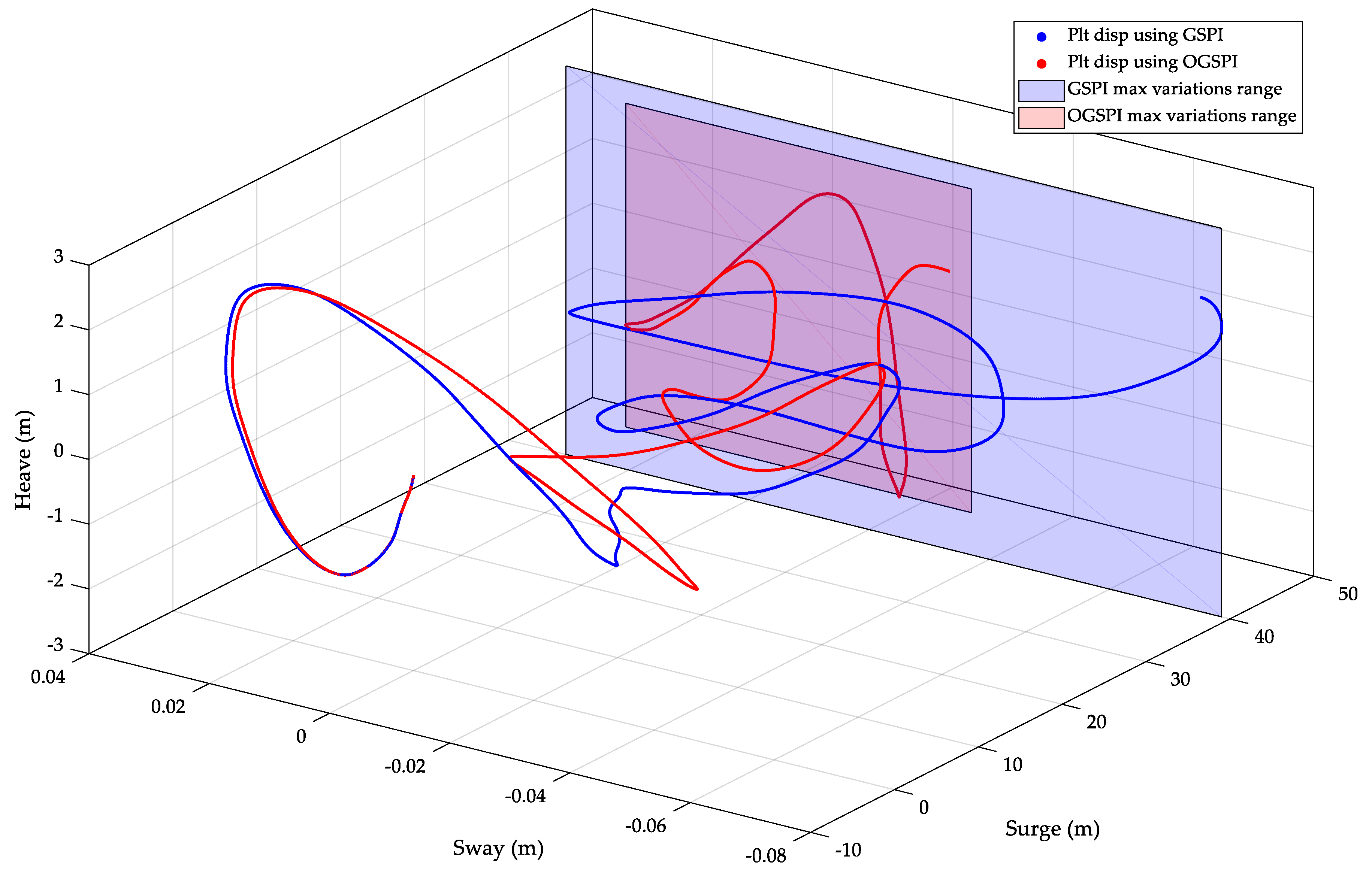
• Proposed a self-tuning improved version of the GSPI that reduces platform movement by more than 50%.
• Using the grey wolf optimizer (GWO) [17] algorithm intelligence, the OGSPI parameters are obtained with low effort.

According to the principles of the “no-free lunch” hypothesis, the success of a metaheuristic optimizer cannot be anticipated [17]. As a result, various metaheuristic optimizers are used in this study to compare their performance to that of the GWO. The used algorithms for the comparison are Harris hawks optimization (HHO) [18], African vultures optimization algorithm (AVOA) [19], COOT optimization algorithm [20], sine cosine algorithm (SCA) [21], and whale optimization algorithm (WOA) [21]. Compared with GWO, which uses the best three solutions to drive the optimization process, each of the previously mentioned algorithms has several characteristics. AVOA uses the two best algorithm solutions to represent the two groups of eagles stronger than the others. This makes a balance between diversity and resonance. This AVOA is more flexible and has less computational complexity, but it was not able to perform well when dealing with more complex problems. Regarding the COOT algorithm, the optimization process is carried out by a lead group. Multiple leading points will enhance the exploration ability with low computational efforts. However, the accuracy of the guiding mechanism is relatively weak compared to other algorithms. The SCA algorithm updates the candidate solutions based on the best-obtained solution as the target point. The SCA algorithm’s search agents are able to diverge and converge thanks to several random and adaptive factors. This can enhance its accuracy but needs more calculation time. The HHO is a more advanced optimization algorithm that controls the exploitation and exploration phases based on a transition factor. The authors focused on enhancing exploration ability to converge to the optimal solution with the lowest possible iterations. However, this requires more elapsed time per iteration, which increases the total calculation time.

The remainder of this work is structured as follows: The system models employed in this investigation, including the aerodynamic, mechanical, and electrical components, are presented in Section 2. Section 3 depicts the suggested control system’s technique. Section 4 shows the results of the co-simulation between MATLAB/Simulink and OpenFAST. Section 5 of this study presents the conclusions.

2. System Modeling

2.1. Aerodynamic Model

The turbine blades gather aerodynamic (kinetic wind) power and convert it to mechanical power by spinning the LSS. The captured aerodynamic power (P_aer) may be obtained as follows [22]:

$$P_{aer}=\frac{Cp\left(\beta ,\lambda \right)}{2}\rho \pi R^2{V}^3$$

(1)

where V is the wind speed, Cp is the power coefficient, β inclination angle, λ tip–speed ratio, R is the radius, and ρ (=1.225) is the air density. The aerodynamic torque (T_aer) can be expressed as a function of the aerodynamic power and the low-speed shaft (ω_rot) as follows:

$$T_{aer}=\frac{P_{aer}}{{\omega }_{rot}}=\frac{Cp\left(\beta ,\lambda \right)}{2\lambda }\rho \pi R^3{V}^2$$

(2)

$$\lambda =\frac{R{\omega }_{rot}}{V}$$

(3)

where λ tip–speed ratio, R is the radius, ω_rot is the low-speed shaft, and V is the wind speed. The applied loads on the blades that may cause the deformation of the blades are neglected.

2.2. Mechanical Model

According to [23], the mechanical model for the wind turbine adopts a two-mass arrangement, which includes the gearbox mass and the wind wheel mass. This two-mass drivetrain model’s mathematical formulae are based on the principles of Newton’s second law. The dynamics of the low-speed shaft may be stated as follows:

$$J_{rot}\frac{d{\omega }_{rot}}{dt}=T_{aer}-T_{mec}-{\omega }_{rot}{D}_{rot}$$

(4)

where J_rot is the turbine’s rotor shaft inertia, D_rot is the rotor damping constant that expresses the rotor torsional damper that helps in eliminating the vibrations (Nm/(rad/s)), and T_mec is mechanical torque, which can be calculated as follows:

$$T_{mec}=k_s\left({\theta }_{rot}-{\theta }_{gen}\right)+k_d\left({\omega }_{rot}-{\omega }_{gen}\right)=k_s{\theta }_r+k_d{\dot{\theta }}_r$$

(5)

where ω_gen is the generator speed, k_s is the drivetrain stiffness constant, k_d is the damping constant, and θ_r is the angle between the turbine rotor and the generator rotor.

The generator dynamics can be presented as follows:

$$J_{gen}\frac{d{\omega }_{gen}}{dt}=\frac{T_{mec}}{{\eta }_g}-T_{em}-{\omega }_{gen}{D}_{gen}$$

(6)

where J_ger is the generator shaft inertia, T_em is electromagnetic torque, D_gen is the generator self-damping coefficient, and η_g is the gear ratio. Neglecting all the damping and stiffness factors, Equation (6) can be rewritten as follows:

$$J_{gen}\frac{d{\omega }_{gen}}{dt}=\frac{1}{{\eta }_g}\left(T_{aer}-J_{rot}\frac{d{\omega }_{rot}}{dt}\right)-T_{em}=\frac{1}{{\eta }_g}\left(T_{aer}-J_{rot}\frac{1}{{\eta }_g}\frac{d{\omega }_{gen}}{dt}\right)-T_{em}=\frac{T_{aer}}{{\eta }_g}-\frac{J_{tr}}{{\eta }_g{}^2}\frac{d{\omega }_{gen}}{dt}-T_{em}$$

(7)

$$\left(J_{gen}+\frac{J_{rot}}{{\eta }_g{}^2}\right)\frac{d{\omega }_{gen}}{dt}=\frac{T_{aero}}{{\eta }_g}-T_{em}$$

(8)

2.3. Electric Model

The electrical equations of the stator and the rotor of PMSG in the direct–quadratic (DQ) axes are written [24]:

$$v_d=R_s{i}_d+L_d\frac{d{i}_d}{dt}-{\mathsf{\Omega }}_e{L}_q{i}_q$$

(9)

$$v_q=R_s{i}_q+L_q\frac{d{i}_q}{dt}+{\mathsf{\Omega }}_e\left({\psi }_s+L_d{i}_d\right)$$

(10)

where L_d and Lq are the direct and quadratic inductance values, is the stator flux, Ω_e is the electrical speed that can be expressed as a function of θ or as a function of ωHSS and the number of the poles of the machine (p). The mechanical equations of electromagnetic torque where p is the number of poles on the machine, L_d and L_q are the direct and quadratic inductance values, ψ_s is the stator flux, and Ω_e is the electrical speed, which may be represented as a function of ω_gen.

The electromagnetic torque’s mechanical equations:

$$T_{em}=\frac{3p}{2}\left(i_d{i}_q\left(L_d-L_q\right)+{\psi }_s{i}_q\right)$$

(11)

3. The Control System

The controller’s primary goals are to maintain power production at the rated value when wind speeds exceed the rated threshold and to maximize power generation when wind speeds exceed the cut-in threshold. Figure 2 illustrates this operating approach.

To manage the generated power, the generator torque has to be adjusted. The generator requires six control zones to achieve this, as shown in Figure 2:

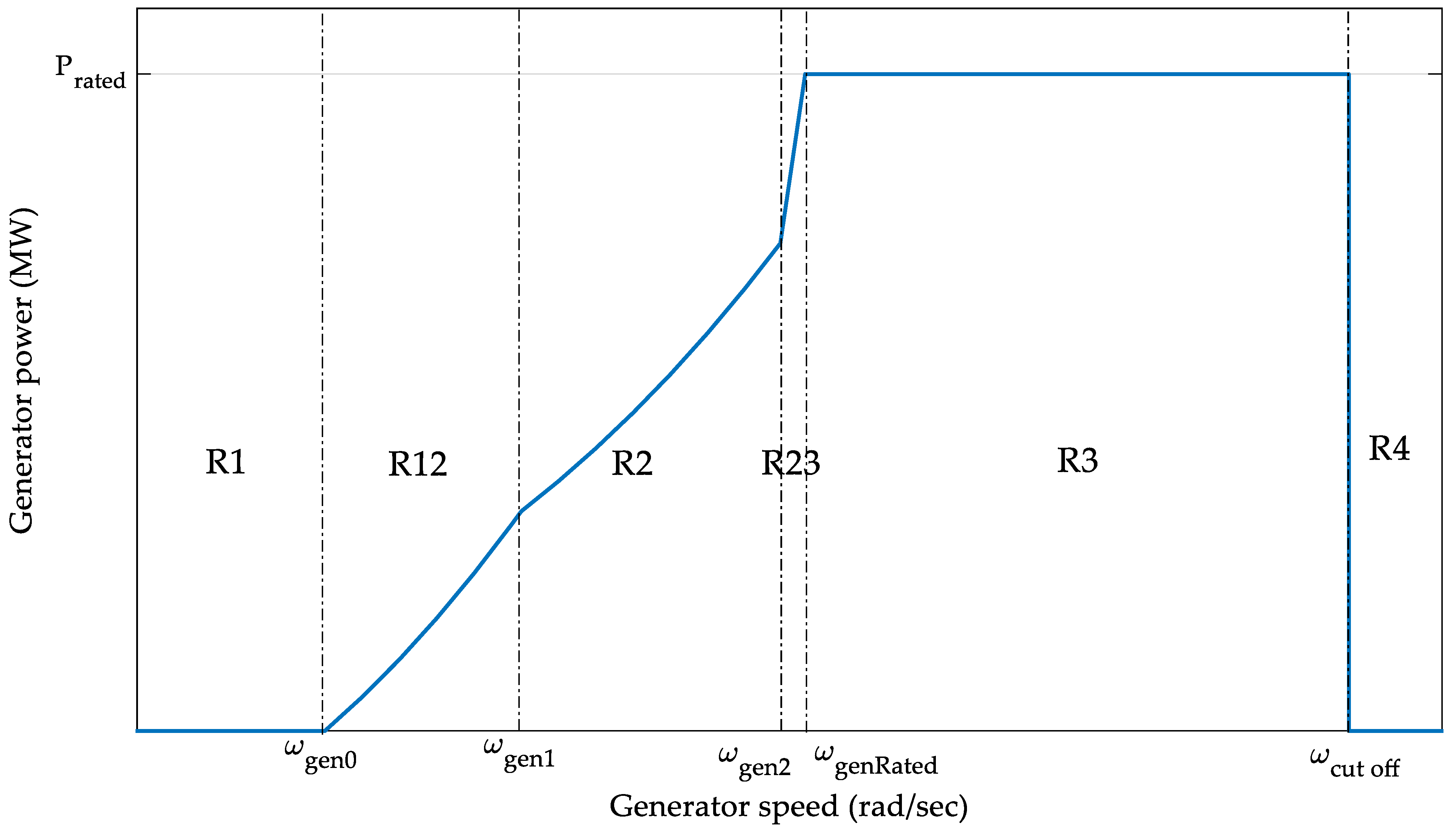
• Region 1: the generator speed is below the starting value (ωgen0), the generator torque is zero, and no power is collected. Instead, the wind is utilized to speed the rotor during the start-up process.
• Region 2: the generator torque is proportional to the square of the generator speed, which is between the transitional generator speed between R12 and R2 (ωgen1) and the transitional generator speed between R2 and R23 (ωgen2). The control technique in this area should employ an MPPT method to optimize the produced power. The torque expression can be expressed as follows:

$$T_{em}=k_{mppt}{\omega }_{gen}{}^2$$

(12)

• where k_mppt is the MPPT gain.
• Region 12: when linear transit is provided between R1 and R12, the generator speed is linearly limited between ω_gen0 and ω_gen1.

$$T_{em}=S_1\left({\omega }_{gen}-{\omega }_{gen0}\right)$$

(13)

$$S_1=\frac{k_{mppt}{\omega }_{gen1}{}^2}{{\omega }_{gen1}-{\omega }_{gen0}}$$

(14)

• Region 3: because the power must be kept constant at the rated generator speed (ω_genRated), the torque is inversely proportional to the generator speed.

$$T_{em}=\frac{P_{rated}}{{\omega }_{gen}}$$

(15)

• where P_rated is the rated generator power.
• Region 23: the generator speed is linearly limited to the tip –speed of rated power between ω_gen2 and ω_genRated.

$$T_{em}=S_2\left({\omega }_{gen}-{\omega }_{gen2}\right)$$

(16)

$$S_2=\frac{\raisebox{1ex}{$P_{rated}$}\!\left/ \!\raisebox{-1ex}{${\omega }_{genRated}$}\right.}{{\omega }_{genRated}-{\omega }_{gen2}}$$

(17)

• Region 4: if the wind speed exceeds the cut-off value (ω_{cut off}), the wind turbine is deactivated in order to safeguard itself.

Concentrating on Region 3, when the power coefficient (Cp) changes with the blade pitch angle (β), the wind turbine blades can achieve aerodynamic productivity. In actuality, regulating the blade pitch angle in Region 3 for FOWTs has two unique purposes: reducing floating platform movements and regulating power [25,26]. Most commercial FOWTs use a typical PI controller to reduce the error between the rotor speed and the rated value [27].

3.1. PI Controller

The PI controller can generate the required pitch angle variations (Δβ_ref) based on the calculated k_p and k_i parameters and the error value between the reference power and the measured reference. Based on the recommendation in ref. [28], the control gains can be obtained as follows:

$$k_p=\frac{2\zeta {\omega }_n{J}_{mec}{\omega }_{genRated}}{{\eta }_g{}^2\left(-\frac{\partial P_{aer}}{\partial \beta }\right)}$$

(18)

$$k_i=\frac{{\omega }_n{}^2{J}_{mec}{\omega }_{genRated}}{{\eta }_g{}^2\left(-\frac{\partial P_{aer}}{\partial \beta }\right)}$$

(19)

where ω_n is the natural frequency and ζ is the damping factor.

3.2. Gain-Scheduled PI (GSPI) Controller

Because of the nonlinearity of the wind turbines, the operating point is continually shifting. Consequently, the rate performance cannot be satisfied by the current control parameters, and a gain-scheduling correction is introduced to change the parameters per the operating point. According to ref. [29], the PI gains alter linearly as the pitch angle changes. As a result, the control equation may be expressed as follows:

$$∆{\beta }_{ref}=GS\left(\beta \right)\left(k_{p}e\left(t\right)+k_i\int e\left(t\right)dt\right)$$

(20)

$$GS\left(\beta \right)=\frac{1}{1+\raisebox{1ex}{$\beta $}\!\left/ \!\raisebox{-1ex}{${\beta }_k$}\right.}$$

(21)

where β_k is the pitch angle where the pitch angle sensitivity value doubles from the rated operating point.

3.3. The Proposed Controller

Metaheuristic optimization techniques are frequently used to solve challenging optimization problems like optimizing control parameters. Physical processes inspire these algorithms, including evolution, swarm behavior, and natural occurrences. They thoroughly search the search space to find the finest or nearly ideal solution. The grey wolf optimizer (GWO) is a popular metaheuristic algorithm. The GWO algorithm simulates gray wolves’ natural leadership structure and hunting mechanism [17]. The leadership hierarchy is simulated using four sorts of grey wolves: alpha, beta, delta, and omega. In addition, three key hunting processes are incorporated to optimize performance: seeking, surrounding, and attacking prey. The mathematical model for each step can be represented as follows:

3.3.1. Encircling Prey

$$P_W\left(t+1\right)=P_P\left(t\right)-A·D\left(t\right)$$

(22)

$$D\left(t\right)=\left|C·P_P\left(t\right)-P_W\left(t\right)\right|$$

(23)

where P_W is the wolves’ positions, P_P is the prey’s position, t denotes the iterations, and A and C are vectors that contain the adaptive control gains.

3.3.2. Hunting Prey

$$P_W\left(t+1\right)=\frac{P_{W1}\left(t\right)+P_{W2}\left(t\right)+P_{W3}\left(t\right)}{3}$$

(24)

$$\left\{\begin{array}{c}{P}_{W1}\left(t\right)=P_{\alpha }\left(t\right)-A_1·D_{\alpha }\left(t\right)\\ P_{W2}\left(t\right)=P_{\beta }\left(t\right)-A_2·D_{\beta }\left(t\right)\\ P_{W3}\left(t\right)=P_{\delta }\left(t\right)-A_3·D_{\delta }\left(t\right)\end{array}\right.$$

(25)

$$\left\{\begin{array}{c}{D}_{\alpha }\left(t\right)=\left|C_1·P_{\alpha }\left(t\right)-P_W\left(t\right)\right|\\ D_{\beta }\left(t\right)=\left|C_2·P_{\beta }\left(t\right)-P_W\left(t\right)\right|\\ D_{\delta }\left(t\right)=\left|3·P_{\delta }\left(t\right)-P_W\left(t\right)\right|\end{array}\right.$$

(26)

Figure 3 illustrates the evolution of the agents (the wolves) in a bidirectional search space as a function of the iterations.

4. Results and Discussion

This study investigates the NREL 5MW ITI barge floating offshore wind turbine (FOWT). The authors use a co-simulation strategy, integrating MATLAB/SIMULINK and OpenFAST software to simulate all possible degrees of freedom (DOFs) in the system. Figure 4 depicts an exemplary depiction of the simulation framework. OpenFAST comprises several sub-codes, each corresponding to a different wind turbine component and interacting with different influencing forces. The operations of OpenFAST are primarily regulated by the interaction of aerodynamic thrust and hydrodynamics caused by marine waves.

The FAST NREL 5MW baseline configuration with the ITI barge setup was used to obtain aerodynamic and mechanical characteristics. The wind speed was constantly higher than the turbine’s rated value of 13 m/s. The spectrum of the JONSWAP (Joint North Sea Wave Observation Project) was also utilized to produce wave characteristics [30]. This spectrum is especially intriguing because it may reflect nonlinear interactions between waves across extended timeframes and distances. The following is the computation procedure for the JONSWAP spectrum:

$$S_j\left(2\pi f\right)=\frac{\alpha g^2}{{\left(2\pi \right)}^4{f}^5}{e}^{\left(-\frac{5}{4}{\left(\frac{f}{f_p}\right)}^{-4}\right){\gamma }^b}$$

(27)

$$b=e^{\left(-\frac{1}{2{\sigma }^2}{\left(\frac{f}{f_p}-1\right)}^2\right)}$$

(28)

$$\sigma =\left\{\begin{array}{c}\begin{array}{cc}0.07f& f<f_p\end{array}\\ \begin{array}{cc}0.09f& f\ge f_p\end{array}\end{array}\right.$$

(29)

where f is the wave frequency (Hz), α = 8.1 × 10⁻³, g is the gravity acceleration (=9.8 m/s²), f_p is the significant wave height ‘Hs’ peak frequency (Hz), and γ = 3.3.

Table 1. Simulation parameters.

Parameter	Symbol	Value	Unit
Turbine parameters (NREL 5MW ITI energy barge)
The radius of wind turbine	R	63	m
Air density	ρ	1.225	kg/m3
Optimal tip–speed ratio	λopt	9.7
Wind turbine inertia moment	Jtr	115,926	kg.m2
Maximum power coefficient	Cpmax	0.465
Wind cut in speed	Vcut_in	3	m/s
Wind rated speed	Vrated	11.4	m/s
Wind cut out speed	Vcut_out	25	m/s
Generator reference speed	ωref	1173.7	rpm
MPPT gain	kmppt	2.8805
Drivetrain parameters (NREL 5MW ITI energy barge)
Gearbox ratio	n	97
Drivetrain torsional spring	ks	8.67637 × 108	Nm/rad
Drivetrain torsional damper	kd	6.215 × 106	Nm/(rad/s)
Environmental conditions
Significant wave height	Hs	5	m
Peak frequency of the significant wave height	fp	12.4	Hz
Wind speed	Vw	13	m/s

shows the FOWT settings and meteorological conditions that were employed. The wave curves are illustrated in Figure 5.

The optimization approach in this research employs optimizers with a population size of 20 agents and a maximum number of iterations for 20 iterations. The optimization cycle of each algorithm was repeated five times to enhance the likelihood of obtaining optimal results and to test the resilience of each approach.

4.1. Simulation Results Comparison

Table 2 highlights the optimization technique’s statistical outputs, including the best, worst, mean, and standard deviation (STD) findings. This table describes the results obtained by each algorithm. The best result is the lower one, which indicates the best performance of the corresponding set of parameters. The worst corresponds to the higher fitness, meaning that the corresponding set of parameters performed worst. The mean value expresses the average performance, and the standard deviation (STD) indicates the algorithm’s robustness. All these indicators should be considered to evaluate the performance of each algorithm. From these results, the following observations can be drawn:

• GWO provided the best result (lower fitness value) of 169.964, outperforming all the other algorithms, including HHO with a result of 169.976 and WOA with a result of 170.341.
• The GWO algorithm showed good robustness, as demonstrated by a standard deviation (STD) of 3.913. This is confirmed by the mean value (170.423) and max value (171.035), which are close to the best result (169.964). The COOT also provided a good STD indicator at 4.726. However, the mean value is relatively significant, meaning the COOT is trapped in a local solution.
• The GWO provided the best motion reduction ratio (16.118), which approves its contribution to finding the best parameters for reducing the platform motions.
• Compared to the best outcomes produced by each algorithm (except for the AVOA), the total of the square platform motions acquired by the traditional GSPI approach is 203.170, which is much higher. These results clearly highlight a significant difference between the classical GSPI method and the OGSPI provided by the metaheuristic optimization algorithms.

Table 2. Statistical simulation results.

	AVOA	COOT	HHO	SCA	WOA	GWO
Best	174.860	171.984	169.976	172.982	170.341	169.964
Worst	303.036	183.337	219.602	224.354	235.826	171.035
Mean	220.961	175.095	180.612	187.261	184.147	170.423
STD	52.901	4.726	21.808	21.141	28.896	3.913
Best kp	0.0104767	0.0092126	0.0096815	0.0088913	0.0107274	0.0093141
Best ki	0.0176733	0.0166215	0.0176835	0.0153915	0.0197864	0.0171811
η (%)	−8.757	13.818	11.10	7.8304	9.363	16.118

Table 2. Statistical simulation results.

	AVOA	COOT	HHO	SCA	WOA	GWO
Best	174.860	171.984	169.976	172.982	170.341	169.964
Worst	303.036	183.337	219.602	224.354	235.826	171.035
Mean	220.961	175.095	180.612	187.261	184.147	170.423
STD	52.901	4.726	21.808	21.141	28.896	3.913
Best kp	0.0104767	0.0092126	0.0096815	0.0088913	0.0107274	0.0093141
Best ki	0.0176733	0.0166215	0.0176835	0.0153915	0.0197864	0.0171811
η (%)	−8.757	13.818	11.10	7.8304	9.363	16.118

η is the motion reduction ratio that can be calculated as follows:

$$\eta =\left(f_{GSPI}-f_{mean}\right)/f_{GSPI}$$

(30)

where f_GSPI is the sum of squared platform motions attained through the classical GSPI controller and f_mean is the mean of squared platform motions achieved by each optimizer to assess its average performance.

Figure 6 depicts the fitness progression of several algorithms based on their mean fitness values and convergence speed. This graph shows how the algorithms’ performance varies through optimization cycles. When compared to the other methods, the GWO algorithm has a quicker convergence curve from the curves. This means that the GWO algorithm can arrive at optimal or near-optimal solutions quickly. The GWO algorithm utilizes a three-point leading technique. These leading points will most likely guide the algorithm’s search across the solution space.

4.2. Computational Complexity Analysis

The computational complexity of the methods utilized is investigated to compare their performances. The algorithm’s time complexity quantifies how long the algorithm takes to find the optimal solutions. Three parameters are set in the case of time complexity: population size (N_pop), search space dimensions (D), and number of iterations (T_max).

Table 3. The time complexity of each algorithm.

Parameter	Complexity for a Single Iteration	Complexity for All Iterations	Elapsed Time (s)
AVOA	O(Npop,D)	O(Npop,D,Tmax)	298.44
COOT	O(Npop,D)	O(Npop,D,Tmax)	777.52
HHO	O(Npop,D)	O(Npop,D,Tmax)	2947.40
SCA	O(Npop,D)	O(Npop,D,Tmax)	1594.34
WOA	O(Npop,D)	O(Npop,D,Tmax)	1544.83
GWO	O(Npop,D)	O(Npop,D,Tmax)	1192.00

displays the time complexity comparison results.

From this table, the degree of complexity mainly depends on the population size, the search space dimension, and the maximum number of iterations. However, it can be noted that the GWO required a large amount of computing time for its updating mechanism.

4.3. OGSPI vs. Classical GSPI

Figure 7 displays the acquired pitch angle in proportion to the wave elevation for both the OGSPI and the GSPI techniques. The graph clearly shows the significant difference in pitch corrections made using the OGSPI and GSPI techniques. This comparison demonstrates optimization’s significant effect on pitch angle accuracy.

Figure 8 depicts the power curves in relation to their influence on produced power. In terms of electricity generation, these numbers support the distinction between the OGSPI and the GSPI. The OGSPI improved power generation by providing 63.9496 kWh of energy throughout the simulation duration, whereas the GSPI generated 63.1237 kWh under the same conditions.

Regarding the platform motions, Figure 9 in the right displays the inclinations of the platform using the GSPI controller for each axis: yaw, pitch, and roll. On the other hand, Figure 9 in the left portrays the platform inclinations using the proposed OGSPI. From these figures, it can be seen that the proposed OGSPI successfully decreased the floating platform’s pitch angle. In addition, the roll has also been reduced. This confirms its ability to handle the platform inclinations better.

Acting on the platform inclinations will lead to reducing the platform motions. The motions of the platform center of gravity (surge (x), sway (y), and heave (z)) are illustrated in Figure 8. Of these motions, sway stands out as particularly significant, as it reflects the changes in the platform’s pitch. Based on these figures, the OGSPI method demonstrated a notably improved reduction in platform motions compared to the GSPI approach. This is apparent from the more confined range of variations in sway motions depicted in Figure 8. Furthermore, a discernible reduction in the platform’s pitch angle can be observed in Figure 10 providing clear evidence of GSPI’s superior capability in mitigating motions compared to the conventional GSPI method.

The above results prove the OGSPI-based RTH’s capability to increase power generation while decreasing platform movements. Reducing the platform motion will reduce the applied loads on the WT body, reduce structure fatigue, increase the lifespan of the whole structure, and reduce maintenance costs [31]. For this reason, it is necessary to reduce these motions. In addition, these motions can lead to fluctuation in the output power, consequently affecting the electrical efficiency of the WT. This can be mitigated when these motions are attenuated.

5. Conclusions

The efficiency of floating offshore wind turbines (FOWTs) is substantially impacted by platform vibrations, making platform motion stabilization a vital problem for enhancing their performance. The technique of addressing this issue using gain-scheduled proportional integrator (GSPI) control has received much attention. Nonetheless, this strategy necessitates significant calculations and depends on assumptions, limiting its usefulness. An optimum GSPI (OGSPI) technique can be used to improve performance. This entails using metaheuristic optimization methods to set control parameters, which results in higher performance efficiency for platform movements and power generation. Because of its unique search method, the grey wolf optimizer (GWO) was utilized in this investigation. Its efficiency was confirmed by comparing its performance to other metaheuristic optimization techniques. The simulation results show that the proposed method reduces platform motion while increasing produced power when compared to the classical GSPI, with the sum square of platform motions reduced from 203.170 using the GSPI to 169.964 using the OGSPI via a reduction ratio of 16.118%. However, the electricity produced increased from 63.1237 kWh to 63.9496 kWh in 50 s. In addition, the final findings show that, compared to those caused by the conventional GSPI, the suggested OGSPI may successfully minimize platform motion by 50.48%. However, the proposed controller is based on the GWO. According to the no-free-lunch theory, better control gains may be obtained using other metaheuristic optimization algorithms. On the other hand, the proposed method obtained the gains via an offline optimization process. An online adaptation may provide better performance, but its implementation complexity will increase. Moreover, unlike GSPI, OGSPI is sensitive to platform type. Therefore, OGSPI parameters are designed for each type separately and cannot be applied to all types of platforms.

References

1. Barooni, M.; Ashuri, T.; Velioglu Sogut, D.; Wood, S.; Ghaderpour Taleghani, S. Floating Offshore Wind Turbines: Current Status and Future Prospects. Energies 2022, 16, 2. [Google Scholar] [CrossRef]
2. Barthelmie, R.J.; Larsen, G.C.; Pryor, S.C. Modeling Annual Electricity Production and Levelized Cost of Energy from the US East Coast Offshore Wind Energy Lease Areas. Energies 2023, 16, 4550. [Google Scholar] [CrossRef]
3. O’Kelly, B.C.; Arshad, M. Offshore Wind Turbine Foundations—Analysis and Design. In Offshore Wind Farms; Elsevier: Amsterdam, The Netherlands, 2016; pp. 589–610. [Google Scholar]
4. Mills, S.B.; Bessette, D.; Smith, H. Exploring Landowners’ Post-Construction Changes in Perceptions of Wind Energy in Michigan. Land Use Policy 2019, 82, 754–762. [Google Scholar] [CrossRef]
5. Schallenberg-Rodríguez, J.; García Montesdeoca, N. Spatial Planning to Estimate the Offshore Wind Energy Potential in Coastal Regions and Islands. Practical Case: The Canary Islands. Energy 2018, 143, 91–103. [Google Scholar] [CrossRef]
6. Filgueira-Vizoso, A.; Cordal-Iglesias, D.; Puime-Guillén, F.; Lamas-Galdo, I.; Martínez-Rubio, A.; Larrinaga-Calderón, I.; Castro-Santos, L. Sensitivity Study of the Economics of a Floating Offshore Wind Farm. The Case Study of the SATH® Concrete Platform in the Atlantic Waters of Europe. Energy Rep. 2023, 9, 2604–2617. [Google Scholar] [CrossRef]
7. Kaldellis, J.K.; Apostolou, D. Life Cycle Energy and Carbon Footprint of Offshore Wind Energy. Comparison with Onshore Counterpart. Renew. Energy 2017, 108, 72–84. [Google Scholar] [CrossRef]
8. Yang, C.; Jia, J.; He, K.; Xue, L.; Jiang, C.; Liu, S.; Zhao, B.; Wu, M.; Cui, H. Comprehensive Analysis and Evaluation of the Operation and Maintenance of Offshore Wind Power Systems: A Survey. Energies 2023, 16, 5562. [Google Scholar] [CrossRef]
9. Faraggiana, E.; Sirigu, M.; Ghigo, A.; Bracco, G.; Mattiazzo, G. An Efficient Optimisation Tool for Floating Offshore Wind Support Structures. Energy Rep. 2022, 8, 9104–9118. [Google Scholar] [CrossRef]
10. Grasu, G.; Liu, P. Risk Assessment of Floating Offshore Wind Turbine. Energy Rep. 2023, 9, 1–18. [Google Scholar] [CrossRef]
11. Sang, L.Q.; Li, Q.; Maeda, T.; Kamada, Y.; Huu, D.N.; Tran, Q.T. Sanseverino, ER Study Method of Pitch-Angle Control on Load and the Performance of a Floating Offshore Wind Turbine by Experiments. Energies 2023, 16, 2762. [Google Scholar] [CrossRef]
12. Jonkman, J. Influence of Control on the Pitch Damping of a Floating Wind Turbine. In Proceedings of the 46th AIAA Aerospace Sciences Meeting and Exhibit, Reston, VA, USA, 7 January 2008. [Google Scholar]
13. Bagherieh, O.; Nagamune, R. Gain-Scheduling Control of a Floating Offshore Wind Turbine above Rated Wind Speed. Control Theory Technol. 2015, 13, 160–172. [Google Scholar] [CrossRef]
14. Schlipf, D.; Simley, E.; Lemmer, F.; Pao, L.; Cheng, P.W. Collective Pitch Feedforward Control of Floating Wind Turbines Using Lidar. J. Ocean Wind Energy 2015, 2, 223–230. [Google Scholar] [CrossRef]
15. Mendoza, N.; Robertson, A.; Wright, A.; Jonkman, J.; Wang, L.; Bergua, R.; Ngo, T.; Das, T.; Odeh, M.; Mohsin, K.; et al. Verification and Validation of Model-Scale Turbine Performance and Control Strategies for the IEA Wind 15 MW Reference Wind Turbine. Energies 2022, 15, 7649. [Google Scholar] [CrossRef]
16. Jonkman, J.M.; Buhl, M.L. FAST Users Guide NREL; National Renewable Energy Lab.: Golden, CO, USA, 2005. [Google Scholar]
17. Mirjalili, S.; Mirjalili, S.M.; Lewis, A. Grey Wolf Optimizer. Adv. Eng. Softw. 2014, 69, 46–61. [Google Scholar] [CrossRef]
18. Heidari, A.A.; Mirjalili, S.; Faris, H.; Aljarah, I.; Mafarja, M.; Chen, H. Harris Hawks Optimization: Algorithm and Applications. Futur. Gener. Comput. Syst. 2019, 97, 849–872. [Google Scholar] [CrossRef]
19. Abdollahzadeh, B.; Gharehchopogh, F.S.; Mirjalili, S. African Vultures Optimization Algorithm: A New Nature-Inspired Metaheuristic Algorithm for Global Optimization Problems. Comput. Ind. Eng. 2021, 158, 107408. [Google Scholar] [CrossRef]
20. Naruei, I.; Keynia, F. A New Optimization Method Based on COOT Bird Natural Life Model. Expert Syst. Appl. 2021, 183, 115352. [Google Scholar] [CrossRef]
21. Mirjalili, S. SCA: A Sine Cosine Algorithm for Solving Optimization Problems. Knowl. Based Syst. 2016, 96, 120–133. [Google Scholar] [CrossRef]
22. Guenoune, I.; Plestan, F.; Chermitti, A.; Evangelista, C. Modeling and Robust Control of a Twin Wind Turbines Structure. Control Eng. Pract. 2017, 69, 23–35. [Google Scholar] [CrossRef]
23. Hu, S.; Song, B. Optimal Control Strategies of Wind Turbines for Load Reduction. In Modeling and Modern Control of Wind Power; Wiley: Hoboken, NJ, USA, 2017; pp. 63–83. [Google Scholar]
24. Afsharnia, S. Contrôle Vectoriel Des Machines Synchrones à Aimants Permanents: Identification Des Paramètres et Minimisation Des Ondulations de Couple. Ph.D. Thesis, Institut National Polytechnique de Lorraine, Nancy, France, 2018. [Google Scholar]
25. Tiwari, R.; Babu, N.R. Recent Developments of Control Strategies for Wind Energy Conversion System. Renew. Sustain. Energy Rev. 2016, 66, 268–285. [Google Scholar] [CrossRef]
26. Navarrete, E.C.; Trejo Perea, M.; Jauregui Correa, J.C.; Carrillo Serrano, R.V.; Moreno, G.J.R. Expert Control Systems Implemented in a Pitch Control of Wind Turbine: A Review. IEEE Access 2019, 7, 13241–13259. [Google Scholar] [CrossRef]
27. Hwas, A.; Katebi, R. Wind Turbine Control Using PI Pitch Angle Controller. IFAC Proc. Vol. 2012, 45, 241–246. [Google Scholar] [CrossRef]
28. Hansen, M.H.; Hansen, A.; Larsen, T.J.; Øye, S.; Sørensen, P.; Fuglsang, P. Control Design for a Pitch-Regulated, Variable Speed Wind Turbine; Riso National Laboratory: Roskilde, Denmark, 2005; Vol. 1500, ISBN 8755034098. [Google Scholar]
29. Jonkman, J.M. Dynamics Modeling and Loads Analysis of an Offshore Floating Wind Turbine; National Renewable Energy Lab.: Golden, CO, USA, 2007. [Google Scholar]
30. Pierson, W.J.; Moskowitz, L. A Proposed Spectral Form for Fully Developed Wind Seas Based on the Similarity Theory of S. A. Kitaigorodskii. J. Geophys. Res. 1964, 69, 5181–5190. [Google Scholar] [CrossRef]
31. Igwemezie, V.; Mehmanparast, A.; Kolios, A. Current Trend in Offshore Wind Energy Sector and Material Requirements for Fatigue Resistance Improvement in Large Wind Turbine Support Structures—A Review. Renew. Sustain. Energy Rev. 2019, 101, 181–196. [Google Scholar] [CrossRef]
Figure 1. Different floating platforms for FOWTs.
Applsci 13 11595 g001
Figure 2. Typical wind turbine power evolution versus wind speed.
Applsci 13 11595 g002
Figure 3. Evolution of an optimization process using the GWO.
Applsci 13 11595 g003
Figure 4. Matlab/Simulink with OpenFast co-simulation platform.
Applsci 13 11595 g004
Figure 5. Wave elevations as a function of the time.
Applsci 13 11595 g005
Figure 6. Average fitness evolution.
Applsci 13 11595 g006
Figure 7. The resulting pitch angle of the OGSPI and the GSPI as a function of the wave elevation.
Applsci 13 11595 g007
Figure 8. The generated power using the OGSPI and the GSPI.
Applsci 13 11595 g008
Figure 9. The platform inclinations using: (right)—GSPI; (left)—OGSPI.
Applsci 13 11595 g009
Figure 10. The platform motions using: blue—GSPI; red—OGSPI.
Applsci 13 11595 g010