Buckling Resistance of Tapered Steel Columns

Abstract

Tapered steel members are widely used in structural and architectural engineering for their efficiency and adaptability, allowing for optimal material usage tailored to specific load levels. However, their complex stability characteristics have hindered their representation in modern design standards like EN 1993 and AISC 360. Existing buckling solutions are limited, and practical research is lacking. This paper comprehensively examines the buckling resistance calculation methodologies for members with variable cross-sections, addressing discrepancies across the methodologies, particularly regarding the tapering ratio. A parametric analysis and numerical simulations were conducted to evaluate each methodology’s applicability, emphasizing the need to balance computational simplicity and accuracy. The study primarily focused on tapered steel beams, considering the different tapering ratios and loading conditions. The findings provide valuable insights into the buckling behavior in tapered members and the practical implications for real-world structural designs. By examining the available analytical methods for calculating the buckling resistance of tapered elements, a better understanding of how to accommodate the non-uniformity of a member was gained, enabling an overview of the variance in the determined resistances and an assessment of the method’s applicability. Moreover, specific calculation methodologies were found to have shortcomings that require modifications for a more accurate parametric analysis. This research contributes to the field by bridging the gaps in modern design standards and enhancing the understanding of buckling in tapered steel members.

1. Introduction

Tapered members (Figure 1), beams, and columns with varying cross-sections are widely used in industrial and high-rise buildings for structural and architectural purposes [1]. Frequently seen in malls, halls, and airports, they are efficient in material usage, adaptable to load levels, and capable of forming various optimal shapes. Commonly used where bending loads are dominant, their designs can be adjusted according to the bending moment diagram. A taper is created by angling a cut on the web of a wide-flange beam, then rotating one segment and joining the webs by welding or by constructing the member directly from steel plates. Timoshenko and Gere [2] also endorsed them for columns, considering buckling-induced bending moments. They are economically viable for compression-loaded members, particularly when significant bending moments must be transferred at the column—beam connection.

The early work on columns with varying cross-sections is linked to Lagrange in 1770 and later Euler. Research on the elastic buckling strength of tapered columns intensified in the 20th century due to Timoshenko [2,3] and Newmark [4], leading to successive approximations for determining critical loads combined with finite difference expressions. This resulted in efficient solutions for determining the column buckling strength. Significant work on steel frames using tapered I-members began with the Column Research Council and Welding Research Council in 1966 [1] as a continuation of the research at Columbia University led by Butler [5,6]. The experimental data from Prawel et al. [7] led to the practical design procedures for tapered columns by Lee et al. [8], using an equivalent uniform member to determine the buckling resistance. This procedure was adopted into the AISC [9] specifications but was removed in 2005 to encourage further development of the guidelines for tapered I-shaped members. A similar approach was studied by Hirt et al. [10] based on the concept of a prismatic column with the same length but with an equivalent moment of inertia.

Experimental studies of I-shaped tapered members grew in subsequent years, with crucial contributions from Salter et al. [11] and Shiomi et al. [12,13], but only for compact members. Forest et al. [14] executed research to evaluate the design provisions made by Star Building Systems and the procedure by Lee et al. [15] concluded that no design provisions accurately predicted the frame resistance for all the loading combinations. The pilot study conducted by White et al. [16] evaluated the AISC [17] stability checks for tapered members, proposing several methods for determining the elastic buckling resistance.

Recent research based on the finite element method (FEM) has shown that using uniform finite elements to analyze members with variable cross-sections (by dividing the member into smaller areas) can lead to significant errors when torsion influences the behavior, as found in the works of Ronagh et al. [18,19] as well as Boissonnade et al. [20].

Baptista et al. [21] were among the first to address the lack of design guidelines for tapered members in EN 1993 [22], proposing a procedure based on the existing provisions for uniform columns. Similar concepts were introduced by Ermopoulos [23], but they were more complex and not readily applicable to EN 1993. Ermopoulos [24] further developed this procedure to include the possibility of encompassing columns with a variable axial force per length.

More recent research on the design of tapered members related to flexural buckling was conducted by Simões da Silva et al. [25] and Marques et al. [26]. They proposed a design procedure for tapered members based on FEM parametric analyses and the general method available in EN 1993-1-1 [22]. Quan et al. [27] proposed an approach which used the geometric and material nonlinearity, considering the imperfections, and defined the member’s ultimate strength by either the strain limit or peak load factor. Bai et al. [28] proposed a generalized imperfection shape function for the practical design of tapered I-section columns, and using this function, a new beam—column element was developed for tapered symmetric I-sections. Abdelrahman et al. [29] proposed generalized line-element formulations for the geometrically nonlinear analysis of tapered steel members with nonsymmetric cross-sections. Chen et al. [30] introduced an analytical model for the second-order direct analysis of steel structures with tapered members, allowing for symmetric and asymmetric variations. Kucukler et al. [31] developed a stiffness reduction method for the in-plane design of web-tapered steel structures fabricated by welding individual plates. Other notable contributions included those by Šapalas et al. [32] and Serna et al. [33], where each introduced new design concepts for tapered members.

Trong-Ha Nguyen et al. [34] developed an artificial neural network model to predict the critical buckling load of the web-tapered I-section steel columns, and the results of the proposed model were compared with approaches according to [8,10,21,26]. The developed model predicted the critical buckling load of the columns more accurately than the existing equations.

Ibrahim [35] and Mahini [36] proposed approaches though which it is possible to determine the buckling length of columns of variable cross-sections by multiplying the length by the K-factor.

As a particular type of tapered structure, acoustic black hole (ABS) structures have been extensively studied recently [37,38,39]. Buckling analyses in structural engineering have seen applications beyond traditional materials and shapes. For instance, recent research [40,41,42,43] presented the mechanical buckling and bending of stiffened functionally graded material (FGM) plates and beams. The studies focused on the influence of the material distribution, thickness-to-width ratio, and stiffener parameters on the buckling characteristics of the stiffened FGM plates and beams. Although this work differed in material composition and configuration, it highlighted the importance of considering various parameters in the buckling analysis, a theme central to the study of tapered steel members. The structural analysis of variable thickness plates with shear connectors has been a subject of interest in recent research.

Despite being used for over 50 years, the design procedures for tapered members are not implemented in modern steel design standards (EN 1993 and AISC 360). Such a state can be attributed to the complexity of describing the stability compared to uniform members due to shifts in the bending, torsional, and axial stiffness with cross-section changes. Analytical solutions for buckling tapered compression members are only available in the elastic area for simple cases. The calculation of non-uniform members’ buckling requires numerical and energy methods. There is a lack of research on practical structural design problems for non-uniform columns, and those that do exist often are not practical enough for everyday engineering use. Considering the complexity and engineering applicability, there is a need for further evaluation of the available design procedures.

The paper describes the available analytical methods for calculating the buckling resistance of tapered elements. Subsequently, a parametric analysis was conducted using the ANSYS 2019 computer program for the selected slenderness and tapering ratios to assess the accuracy of each method. The paper also evaluates the applicability of each method, considering the number of required parameters and the deviation of the calculation results compared to the reference methodology.

2. Available Stability Design Procedures for Tapered Members

2.1. Lee, Morrell, and Ketter [8]

The approach developed by Lee et al. [8] estimates the effective length of a tapered member by changing its length to obtain an equivalent uniform member. The uniform member has the properties of the smallest cross-section of the non-uniform member, and the properties of the newly formed member are then used in the standard Equation (1) for elastic buckling.

$$N_{cr,taper}=\frac{{\pi }^2\cdot E\cdot I_{y,min}}{{\left(g\cdot L\right)}^2}$$

(1)

where N_cr,taper is the critical force of the elastic buckling of the non-uniform member, E is the modulus of elasticity, I_min is the moment of inertia of the smallest cross-section about the stronger axis of the non-uniform element, and gL is the modified length of the uniform member. By rearranging Equation (1), it is possible to obtain the length change factor for a pin-ended member, g, depicted by Equation (2).

$$g=\frac{\pi }{L}\cdot \sqrt{\frac{E\cdot I_{y,min}}{N_{cr,taper}}}$$

(2)

In Equation (2), all the variables are known except for N_cr,taper, and the authors have provided a solution for N_cr,taper for the most commonly used cross-sections. Considering various lengths and degrees of shape change, they arrived at Equation (3) for calculating the length change factor, g.

$$g=1.000-0.375\cdot \gamma +0.080\cdot {\gamma }^2\cdot \left(1.00-0.0775\cdot \gamma \right)$$

(3)

where γ is the degree of non-uniformity (tapering ratio), which considers the ratio of the heights of the largest h_max and smallest cross-section of the element h_min, using Equation (4).

$$\gamma =\frac{h_{max}}{h_{min}}-1$$

(4)

The equation for the length change factor, g, can be determined based on the curve fitting procedure to the representative test results of the members with five different cross-sections. The functional relationship of the length change factor, g, and the degree of non-uniformity, γ, according to Equations (3) and (4), can be determined by a third-degree polynomial. For the values of the tapering ratio γ greater than 7.75, the values of the length change factor become negative. Although such values of the tapering ratio are hard to reach, it is not possible to perform a resistance calculation of a tapered element even for values of the tapering ratio greater than 6.5 due to a pronounced drop in the value of the length change factor with the increase in the degree of non-uniformity, γ. The advantage of the approach is its simplicity of use and the possibility of application in the existing regulatory methodology, thereby simultaneously enables the consideration of imperfections and advancements in this area.

The procedure for implementing the buckling calculation, following the methodology proposed by Lee et al., into the EN 1993 standard flexural buckling design is relatively straightforward as the modification is based on the elastic critical force (Figure 2).

2.2. Baptista and Muzeau [21]

Baptista et al. [21] solved the problem of calculating the buckling resistance of the tapered elements, N_b,taper,Rd, by modifying the existing expression for determining the buckling resistance, according to EN 1993 [22], N_b,Rd, with the coefficient k (Equation (5)), which depends on the slenderness of the member with the smallest cross-section and the degree of non-uniformity (Figure 3 and Figure 4).

$$N_{b,taper,Rd}=k\cdot N_{b,Rd}=k\cdot {\chi }_{min}\frac{A_{min}\cdot f_y}{{\gamma }_{M1}}$$

(5)

where χ_min is a reduction factor that accounts for the loss of stability and imperfections of the element, A_min is the area of the smallest cross-section, f_y is the steel yield strength, and γ_M1 is a partial factor for the stability calculations.

The k-factor is calibrated only up to a specific value of the tapering ratio γ = h_max/h_min, which must not exceed 6.67 for this methodology. A linear interpolation must be performed for all the values of the tapering ratio between the given curves. In addition, for the slenderness values up to 0.6 and after 3.0, the distribution of the k-factor is unknown, which significantly limits the application of the method. This methodology can be considered conservative as the entire calculation is based on the properties of the smallest cross-section, thereby assuming the same yield in all nominal cross-sections along the length of the member. In addition, this methodology’s reliance on graphically determining the factors for an increasing resistance to buckling represents an awkward solution that prevents engineers from fully digitizing the calculations and allows for errors. The advantage of this approach is undoubtedly the relative simplicity of use due to the grounding of the analytical part of the methodology on a normative basis.

2.3. Šapalas, Samofalov i Šaraškinas [32]

Šapalas et al. [32] presented an approach for calculating the non-uniform member subjected to an axial compressive force based on the properties of an equivalent cross-section. Their approach was independent of the standards because the entire calculation uses the standard procedure for a member of the same length as the non-uniform one but with a uniform equivalent cross-section. Specifically, the equivalent height is calculated after calculating the calibration factor, αn, which depends on the ratio of the end moments of inertia of the non-uniform member, I_y,min/I_y,max. This equivalent height is then used to obtain the properties of a replacement uniform element. Figure 5 provides a summarized representation of the described calculation process.

The values of the calibration factor, α_n, as shown in

Table 1. Values of the calibration factor α_n [25].

Iy,min/Iy,max	0.010	0.050	0.100	0.200	0.300	0.400	0.500	0.600	0.700	0.800	0.900	1.000
αn	0.563	0.629	0.676	0.740	0.788	0.829	0.864	0.895	0.924	0.951	0.976	1.000

, were obtained based on the results of the numerical simulations of the buckling of non-uniform compressive members and are based on Equation (6).

$${\left(\frac{\pi }{{\mu }_y\cdot L}\right)}^2\cdot E\cdot I_{y,taper}={\alpha }_n\cdot {\left(\frac{\pi }{{\mu }_y\cdot L}\right)}^2\cdot E\cdot I_{y,max}$$

(6)

where I_y,taper is the moment of inertia of the equivalent member and I_y,max is the moment of inertia of the largest cross-section of the non-uniform element.

Although the calculation of the buckling resistance according to this methodology is based on a section that can be considered critical, the resistance value according to the methodology offered by the standard cannot be greater than the resistance of the smallest cross-section. Therefore, this only extends to the area of non-dimensional slenderness in which the value of the resistance reduction factor equals one. Accordingly, although Šapalas et al. [32] did not mention the calculation process after determining the critical buckling force in their work, the applied methodology (Figure 5) assumes that the equivalent cross-section is used to determine the reduction factor χ, and then the obtained reduction factor is applied to reduce the resistance of the smallest cross-section in the non-uniform member. This way, it is possible to obtain realistic resistance values, considering that the smallest cross-section limits the resistance.

2.4. Smith [44]

Smith [44] described the energy method for calculating non-uniform compressive elements with a regular change in cross-section. In the appendix of his work, Smith [44] provided a display of a factor for adjusting the critical buckling force, factor m, which depends on the ratio of moments of inertia of the smallest and largest cross-sections of the non-uniform element.

According to Smith, following the proposed procedures, the basic expression for the critical force takes the form of Equation (7).

$$N_{cr,taper}=\frac{m\cdot E\cdot I_{y,max}}{L_{}^2}$$

(7)

where m is the factor for adjusting the critical buckling force, I_y,max is the moment of inertia of the largest cross-section, and L is the buckling length of the member around the corresponding axis. After calculating the critical buckling force according to Equation (7), a further procedure for calculating the buckling resistance is performed using the properties of the largest cross-section of the non-uniform member. Figure 6 provides a summarized representation of the calculation process, according to this methodology.

The values of the factor m depending on the ratio of moments of inertia, as proposed by Smith [44], are shown in

Table 2. Values of factor m [28].

Cantilever	Iy,min/Iy,max	0.000	0.100	0.200	0.300	0.400	0.500	0.600	0.700	0.800	0.900	1.000
	m	-	1.202	1.505	1.710	1.870	2.002	2.116	2.217	2.308	2.391	π2/4
Pin-supported element	Iy,min/Iy,max	0.000	0.100	0.200	0.300	0.400	0.500	0.600	0.700	0.800	0.900	1.000
	m	-	4.808	6.020	6.840	7.480	8.008	8.464	8.868	9.232	9.564	π2

.

The fact that Smith [44] offered values for the factor m only to the value of the ratio of the moments of inertia of 0.1 dramatically limits the application of this method. Namely, with the increase in the tapering ratio (h_max/h_min), there is a pronounced increase in the moment of inertia.

The paper [44] did not discuss calculating load-bearing capacity after determining the critical buckling force. The methodology (Figure 6) assumes that the highest cross-section determines the reduction factor χ. The resistance reduction using the calculated reduction factor is then performed based on the smallest cross-section in the non-uniform element. In addition to the fact mentioned in Section 2.4 that the area of the smallest cross-section certainly limits the resistance, this intervention maintains its simplicity. Namely, at higher tapering ratios, the sections of greater heights enter the cross-section class 4. However, their effective area is slightly larger than the area of the smallest cross-section, making resistance gains negligible at the expense of a more complex calculation. In addition, considering that the effective area only extends to the area of slenderness within which it applies, the reduction factor is equal to one or the curve reduction factor/non-dimensional slenderness slightly translates along the axis of non-dimensional slenderness.

2.5. Serna, Ibáñez i López [33]

The approach shown in [33] and depicted in Figure 7 represents a practice-applicable way for addressing the problem of buckling of non-uniform elements, considering that the calculation procedure presented in it also anticipates the possibility of changing the level of axial force along the length of the member. The approach is based on the fact that a non-uniform element loaded with a variable (or uniform) axial force is replaced with a uniform one with the properties of the smallest cross-section, loaded with an equivalent uniform axial force. According to Equation (8), this methodology assumes that the actual critical buckling force of a non-uniformly loaded uniform member is equal to the product of a particular coefficient C and Euler’s critical force.

$$N_{cr,taper}=C\cdot N_E=C\cdot \frac{{\pi }^2\cdot E\cdot I_{y,min}}{L_{}^2}$$

(8)

Coefficient C considers the non-uniformity of the internal compressive force and cross-section and can be calculated using Equation (9).

$$C=\frac{21\cdot N_{max}}{4\cdot \left(N_{x=0}+N_{x=L}\right)+6\cdot \left(N_{x=L/4}+N_{x=3L/4}\right)+N_{max}}$$

(9)

where N_max is the highest level of axial force in the member, N_{x = 0} and N_{x = L} are the levels of axial force at the ends of the member, and N_{x = L/4} and N_{x = 3L/4} are the levels of axial force at L/4 and 3L/4 of the length of the member.

The obtained equation is incorporated into differential equations that describe the elastic buckling of a non-uniform member, based on which the authors arrived at a general Equation (10), which sufficiently describes the influence of the axial force distribution along a non-uniform member.

$$\widehat{N}\left(x\right)=N\left(x\right)\cdot \frac{I_{min}^{\chi }}{I{\left(x\right)}^{\chi }}\cdot \frac{I_{x=0}^{\beta }\cdot I_{x=L/2}^{\gamma }\cdot I_{x=L}^{\beta }}{I_{max}^{\left(2\cdot \beta +\gamma \right)}}$$

(10)

where I_x=0, I_x=L/2, and I_x=L are the moments of inertia in the sections at distances 0, L/2, and L from the smallest cross-section of the member, I_max is the moment of inertia of the largest cross-section along the member, and I_min is the moment of inertia of the smallest cross-section. The coefficients β, χ, and γ represent the correction coefficients, and the authors have obtained a good agreement with the numerical simulations, with values β = 0.30, χ = 0.30, and γ = 0.15.

Therefore, by using Equations (8)–(10), it is possible to calculate the critical buckling force of a non-uniform member with a non-uniform distribution of axial force. For the case when the compressive force in the element is uniform, Equation (9) takes the form of Equation (11).

$$C=\frac{21}{4\cdot \left(c_{x=0}+c_{x=L}\right)+6\cdot \left(c_{x=L/4}+c_{x=3L/4}\right)+c_{max}}$$

(11)

The different c values are coefficients at the corresponding points, following Equation (10) and using Equation (12).

$$c\left(x\right)=\frac{I_{min}^{\chi }}{I{\left(x\right)}^{\chi }}\cdot \frac{I_{x=0}^{\beta }\cdot I_{x=L/2}^{\gamma }\cdot I_{x=L}^{\beta }}{I_{max}^{\left(2\cdot \beta +\gamma \right)}}$$

(12)

While this methodology can cover many buckling cases for non-uniform members, it is a more complex and laborious procedure for determining the resistance of such members. Namely, to reach the part of the procedure where the critical buckling force is determined, it is necessary to perform at least six calculations almost as complex as the methods presented in Section 2.1, Section 2.3 and Section 2.4. This disadvantage can be partially offset because the entire procedure is analytical and can be quickly solved by various algorithms in software packages that are relatively accessible today. In addition, a simple, functional relationship between factor C and the tapering ratio γ allows for a direct insight into how the critical buckling force changes from calculating only a few values of factor C in the area of the tapering ratio γ of interest.

2.6. Marques, Taras, Simões da Silva, Greiner i Rebelo [26]

This method calculates the position of the critical cross-section and performs a buckling calculation of a non-uniform element using its properties. This position depends on the tapering ratio γ and the critical load multiplier α_cr, which require a numerical buckling simulation. The methodology foresees three shifts in the function, describing the critical cross-section’s position. For a smaller slenderness, the critical cross-section is the smallest one, followed by a displacement by increasing non-dimensional slenderness up to a point where the position of the critical cross-section remains constant. The calculation process according to this method is shown in Figure 8.

The calculation methodology is based on the critical load multiplier α_cr, which is precisely the procedure’s biggest drawback. Namely, the analysis of its form (numerical) complicates the calculation procedure compared to those presented so far, as there is no possibility of analytical determination for this parameter. Introducing numerical analysis into the procedure moves away from practical application because easy automation is impossible. It, thus, realistically weakens the possibility of its inclusion in the normative procedure EN 1993-1-1 [22].

3. Parametric Analysis

The literature’s methods for calculating non-uniform element buckling, discussed in the previous chapter, were used here for a parametric analysis to understand the relationship between the solutions for the different parameters. This analysis helps highlight the differences in the calculation methodologies and assess their practical applicability, enabling a qualitative evaluation of each method based on its calculation complexity and relative result accuracy.

The parametric analysis offers an understanding of the buckling resistance in various non-uniform elements, graphically displayed through curves showing the functional relationship between the normalized resistance values and significant parameters. This allows for an evaluation of how varying variables impact a particular calculation method’s applicability. Moreover, the large data set provides insight into the specific methods’ limitations, suggesting ways to broaden their scope and verifying the calculation results with the applied solutions.

3.1. Limitations, Varied Parameters, and Methods of Displaying Results

To make the results of various methods comparable, it was necessary to determine the range of variations of the variables and set certain limitations so that the results would be valid. Accordingly, in the parametric analysis, the following statements were adopted, which were aligned with the notes from [45].

• The change in the height of the web is linear along the length of the member.
• There is no change in the thickness of the cross-section parts or the width of the flange along the length of the member.
• The analyzed members are homogeneous (the web and flange are of the same steel quality).
• If there are class 4 cross-sections within the length of the element, according to [22], their effective area is larger than the area of the smallest cross-section.

The limitations were tied to the calculation methods’ capabilities, with no method defining the change in the flange’s width or how to incorporate that change. As noted in [45], most automation production equipment requires a constant flange width throughout the member’s length, making this limitation somewhat technological. The chosen parameters varied to allow comparability between the methods and to examine the parameters that designers can manipulate when using a non-uniform member. Thus, the design-influenced variables affecting the buckling resistance calculation (slenderness based on the smallest cross-section; ratio of smallest to largest cross-section heights) were chosen for the parametric analysis.

The tapering ratio change was an essential variable, as suggested in all the methodologies in Section 2. The non-dimensional slenderness based on the smallest cross-section was also varied, as it was the only commonality between the different calculation methodologies. It allowed for the calculation of a specific member length based on the smallest cross-section’s characteristics, which was then applicable to all the calculation methods using the equation derived from the Euler’s buckling critical force, as shown in Equation (13).

$$L={\overline{\lambda }}_{0,min}\cdot \pi \cdot i_0\cdot \sqrt{\frac{E}{f_y}}$$

(13)

where λ_0,min is the non-dimensional slenderness based on the smallest cross-section and i₀ is the radius of inertia of the smallest cross-section.

The unalterable parameters throughout the analysis included the initial cross-section shape, steel quality, and production type, as their changes would only linearly translate the resistance/non-dimensional slenderness curve along the resistance axis. For the analysis, the smallest cross-section for all the members was chosen as HEB 300, based on the analyses in [26], the steel quality S235 according to [22], and a welding production process (plated structural elements). The non-dimensional slenderness based on the smallest cross-section λ_0,min was varied in steps up to a maximum value depending on the tapering ratio γ. The tapering ratios ranged from one for a uniform member up to eight, with variation steps increasing progressively. For the tapering ratios from one to 1.75, the slenderness was varied from zero to three, with a step of 0.20. For the tapering ratios from two to eight, the slenderness range increased by one for each increment (e.g., for the tapering ratio γ = 2, the slenderness range was from zero to four), and the step was kept so that within the range from zero to four it was 0.20, and after that 0.50. The member lengths were determined using Equation (14) based on the varied non-dimensional slenderness, as shown in

Table 3. Buckling lengths depending on the non-dimensional slenderness based on the smallest cross-section—HEB 300; S235.

${\overline{\lambda }}_{0,min}$	0.2	0.4	0.6	0.8	1.0	1.2	1.4	1.6	1.8	2.0	2.2	2.4
L [m]	2.46	4.92	7.38	9.84	12.30	14.76	17.22	19.68	22.14	24.60	27.07	29.53
${\overline{\lambda }}_{0,min}$	2.6	2.8	3.0	3.2	3.4	3.6	3.8	4.0	4.5	5.0	5.5	6.0
L [m]	32.0	34.4	36.9	39.4	41.8	44.3	46.7	49.2	55.4	61.5	67.7	73.8
${\overline{\lambda }}_{0,min}$	6.5	7.0	7.5	8.0	8.5	9.0	9.5	10.0	10.5	11.0
L [m]	80.0	86.1	92.3	98.4	104.6	110.7	116.9	123.0	129.2	135.3

.

The total number of calculations and a summarized view of the varied variables (and their combinations) are shown in

Table 4. Varied parameters and the number of calculations.

Calculation Method	Tapering Ratio—γ = hmax/hmin	$\mathbf{Non}-\mathbf{Dimensional} \mathbf{Slenderness} \mathbf{Based} \mathbf{on} \mathbf{the} \mathbf{Smallest} \mathbf{Cross}-\mathbf{Section}—{\overline{\mathit{\lambda }}}_{0,\mathit{m}\mathit{i}\mathit{n}}$	Number of Calculations	Number of Methods	Summary
Lee et al. [8] Modified Lee et al. [8] 1 Baptista et al. [21] 2 Šapalas et al. [32] Smith [44] Serna et al. [33] Marques et al. [26]	1.00	0.0; 0.2; 0.4; 0.6; 0.8; 1.0; 1.2; 1.4; 1.6; 1.8; 2.0; 2.2; 2.4; 2.6; 2.8; 3.0	16	6	96
	1.25		16	6	96
	1.50		16	6	96
	1.75		16	6	96
	2.00	0.0–3.0; 3.2; 3.4; 3.6; 3.8; 4.0	21	6	126
	2.50	0.0–4.0; 4.5; 5.0	23	6	138
	3.00	0.0–4.0; 4.5; 5.0; 5.5; 6.0	25	6	150
	4.00	0.0–4.0; 4.5; 5.0; 5.5; 6.0; 6.5; 7.0	27	6	162
	5.00	0.0–4.0; 4.5; 5.0; 5.5; 6.0; 6.5; 7.0; 7.5; 8.0	29	6	174
	6.00	0.0–4.0; 4.5; 5.0; 5.5; 6.0; 6.5; 7.0; 7.5; 8.0; 8.5; 9.0	31	6	186
	7.00	0.0–4.0; 4.5; 5.0; 5.5; 6.0; 6.5; 7.0; 7.5; 8.0; 8.5; 9.0; 9.5; 10.0	33	6	198
	8.00	0.0–4.0; 4.5; 5.0; 5.5; 6.0; 6.5; 7.0; 7.5; 8.0; 8.5; 9.0; 9.5; 10.0; 10.5; 11.0	35	6	210
					1728

Note ¹: Methodology applied only for the tapering ratios between 7.0 and 8.0. Note ²: Methodology applied only for the tapering ratios between 1.0 and 6.0.

. The variations and individual steps were chosen based on the area of interest and the required accuracy. The tapering ratios were more densely observed from one to three, representing the most likely range in the typical applications, assuming the height of the members was just a few meters. The observed slenderness area was expanded with the increase in the tapering ratio because the resistance drop trend with the increasing tapering ratio translated the resistance curve along the slenderness axis.

Using the Autodesk Robot Structural Analysis, 291 numerical buckling simulations were carried out according to the method by Marques et al. [26] to determine the critical load multiplier α_cr for the varied member cases. Steel was modeled as elastic with a yield strength of 235 N/mm² and a modulus of elasticity of 210.000 N/mm². An additional buckling analysis using shell finite elements confirmed minor differences in the critical load multipliers.

A numerical analysis was also conducted using the ANSYS 2019 software to gain insight into the accuracy of the considered methods for calculating the buckling resistance of the tapered columns. The numerical analysis consisted of two steps. In the first step, an eigenvalue buckling analysis was performed to determine the critical load and to obtain the deformed geometry (initial imperfection) of the tapered member used in the second step, which involved a nonlinear calculation with a gradual increase in the load until failure (Figure 9a). The tapered columns with various slenderness and tapering ratios were modeled using four-node shell elements with six degrees of freedom at each node (SHELL181). At one end of the column, a pinned support was modeled, while on the other side, where the load was applied, a sliding support was modeled, allowing for translation along the member’s longitudinal axis. In the buckling analysis, the steel material was modeled as linear elastic with a modulus of elasticity of 210.000 N/mm². In the nonlinear analysis, the steel was modeled bilinearly with a yield strength of 235 N/mm² and a tangent modulus of 2.100 N/mm². To ensure the accuracy and reliability of the numerical model, we drew upon the meticulously documented, verified, and validated numerical model for tapered steel columns by Marques et al. [26].

3.2. Implementation of the Parametric Analysis

Each procedure from Section 2 was prepared as a calculation sequence for a spreadsheet editor, Microsoft Excel. The methods involving data reading from the curves were mapped and described using regression functions. Some methods were expanded for applicability across the parameter changes range, as shown in Table 4.

The calculation method by Lee et al. [8], which did not require graphical data reading, was ideal for the spreadsheet calculations. However, its applicability was limited by the functional relationship between the change factor length g and the tapering ratio γ per Equation (3). It disallowed the valid buckling resistance for all the parametric analysis-predicted tapering ratios (γ = 7 and 8). Therefore, the application area was expanded to larger tapering ratios by isolating and extending the relatively linear part of the g-γ curve between the tapering ratios 3.0 and 5.5. This maintained the safety of the approach for assessing the resistance of non-uniform members by keeping the new curve above the existing one, and the change was easily incorporated into the existing equation by adding a simple inequality condition that regulated the scope of each function. In this case, Equation (3) took the form of Equation (14).

$$g_{\mathrm{mod}}=1.000-0.375\cdot \gamma +0.080\cdot {\gamma }^2\cdot \left(1.00-0.0775\cdot \gamma \right)\ge -0.0379\cdot \gamma +0.5368$$

(14)

The Baptista et al. [21] method employed curves to read the factor k value, which calculates a non-uniform member buckling resistance. These curves were digitized into regression functions, where the k values read for each prescribed non-dimensional slenderness value from 0.6 to 3.0 (step 0.20) and each ratio from the smallest (h_min) to largest (h_max) cross-section height. The methodology’s scope was expanded for comparison with other methods through the parametric analysis. A relatively linear area around a non-dimensional slenderness of 3.0 to the point of inflexion was used to maintain the capacity increase with the slenderness change. Thus, the functional relationship between k and the slenderness, given by Equations (15)–(21), retained the original form up to a specific slenderness, after which k increased linearly (Figure 10).

$$k\left(0.70\right)=\{\begin{array}{ll}-0.0959\cdot {\overline{\lambda }}_{min}^2+0.4744\cdot {\overline{\lambda }}_{min}^{}+0.9275\hfill & {\overline{\lambda }}_{min}^{}\le 2.4\hfill \\ 0.03\cdot {\overline{\lambda }}_{min}^{}+1.45\hfill & {\overline{\lambda }}_{min}^{}>2.4\hfill \end{array}$$

(15)

$$k\left(0.50\right)=\{\begin{array}{ll}-0.2092\cdot {\overline{\lambda }}_{min}^2+1.095\cdot {\overline{\lambda }}_{min}^{}+0.5853\hfill & {\overline{\lambda }}_{min}^{}\le 2.6\hfill \\ 0.05\cdot {\overline{\lambda }}_{min}^{}+1.9\hfill & {\overline{\lambda }}_{min}^{}>2.6\hfill \end{array}$$

(16)

$$k\left(0.40\right)=\{\begin{array}{ll}-0.261\cdot {\overline{\lambda }}_{min}^2+1.5522\cdot {\overline{\lambda }}_{min}^{}+0.317\hfill & {\overline{\lambda }}_{min}^{}\le 3.0\hfill \\ 0.11\cdot {\overline{\lambda }}_{min}^{}+2.3\hfill & {\overline{\lambda }}_{min}^{}>3.0\hfill \end{array}$$

(17)

$$k\left(0.30\right)=\{\begin{array}{ll}-0.2611\cdot {\overline{\lambda }}_{y,min}^3+1.1828\cdot {\overline{\lambda }}_{y,min}^2-0.2819\cdot {\lambda }_{y,min}+1.0232\hfill & {\overline{\lambda }}_{min}^{}\le 2.8\hfill \\ 0.12\cdot {\overline{\lambda }}_{min}^{}+3.45\hfill & {\overline{\lambda }}_{min}^{}>2.8\hfill \end{array}$$

(18)

$$k\left(0.25\right)=\{\begin{array}{ll}-0.2914\cdot {\overline{\lambda }}_{y,min}^3+1.413\cdot {\overline{\lambda }}_{y,min}^2-0.3931\cdot {\lambda }_{y,min}+1.0148\hfill & {\overline{\lambda }}_{min}^{}\le 3.0\hfill \\ 0.13\cdot {\overline{\lambda }}_{min}^{}+4.3\hfill & {\overline{\lambda }}_{min}^{}>3.0\hfill \end{array}$$

(19)

$$k\left(0.20\right)=\{\begin{array}{ll}-0.3952\cdot {\overline{\lambda }}_{y,min}^3+2.0291\cdot {\overline{\lambda }}_{y,min}^2-1.0354\cdot {\lambda }_{y,min}+1.2067\hfill & {\overline{\lambda }}_{min}^{}\le 3.0\hfill \\ 0.14\cdot {\overline{\lambda }}_{min}^{}+5.3\hfill & {\overline{\lambda }}_{min}^{}>3.0\hfill \end{array}$$

(20)

$$k\left(0.15\right)=\{\begin{array}{ll}-0.4698\cdot {\overline{\lambda }}_{y,min}^3+2.534\cdot {\overline{\lambda }}_{y,min}^2-1.4993\cdot {\lambda }_{y,min}+1.3341\hfill & {\overline{\lambda }}_{min}^{}\le 3.0\hfill \\ 0.15\cdot {\overline{\lambda }}_{min}^{}+6.55\hfill & {\overline{\lambda }}_{min}^{}>3.0\hfill \end{array}$$

(21)

Šapalas et al. [32] used the factor α_n in their methodology to calculate the equivalent height of the member, either graphically or by linear interpolation. Given that linear interpolation could introduce errors in the resistance values and that the graphical method was not ideal for the parametric analyses, a sixth-degree polynomial was used to map the curve describing this relationship. The equation of the curve (22) was directly adopted for the parametric analysis.

$${\alpha }_n=-7.35\cdot \frac{I_y^6\left(x_0\right)}{I_y^6\left(x_L\right)}+24.89\cdot \frac{I_y^5\left(x_0\right)}{I_y^5\left(x_L\right)}-33.14\cdot \frac{I_y^4\left(x_0\right)}{I_y^4\left(x_L\right)}+22.13\cdot \frac{I_y^3\left(x_0\right)}{I_y^3\left(x_L\right)}-8.00\cdot \frac{I_y^2\left(x_0\right)}{I_y^2\left(x_L\right)}+1.92\cdot \frac{I_y^{}\left(x_0\right)}{I_y^{}\left(x_L\right)}+0.55$$

(22)

Smith’s methodology [44] utilized the factor m to adjust the critical buckling force. Given only in table form (Table 2), this factor’s functional relationship with the moments of inertia ratio of a non-uniform member end was a fourth-degree polynomial. As linear interpolation might not have yielded sufficiently accurate results, Equation (23) was adopted for the parametric analysis.

$${\alpha }_n=-9.23\cdot \frac{I_y^4\left(x_0\right)}{I_y^4\left(x_L\right)}+26.28\cdot \frac{I_y^3\left(x_0\right)}{I_y^3\left(x_L\right)}-29.17\cdot \frac{I_y^2\left(x_0\right)}{I_y^2\left(x_L\right)}+18.78\cdot \frac{I_y^{}\left(x_0\right)}{I_y^{}\left(x_L\right)}+3.21$$

(23)

The methodologies proposed by Serna et al. [33] and Marques et al. [26] were well suited to the needs of the parametric analysis in terms of both their scope and calculation method. They were adopted as presented in Section 2.5 and Section 2.6, with the calculations adhering to the procedures shown in Figure 7 and Figure 8, respectively.

4. Comparison of the Results and Discussion

The varied methods used for the analysis allowed for a deeper understanding of how changes in the tapering ratio can impact the resistance of a member. These results also shed light on the discrepancies between the calculated resistances across the different methodologies. By comparing the results of the resistance calculations for each methodology shown in Section 2 on a reduction factor non-dimensional slenderness (χ-λ₀) diagram for each tapering ratio, insights into the trends and the relative accuracy of each methodology were gained. For comparison, the method proposed by Marques et al. [26], based on a large number of numerical analyses incorporating material and geometric imperfections, was used as a reference. This contrasted with other methods primarily based on analytical methods, where imperfections were incorporated via European buckling curves [22]. Along with the results from the observed methodologies, the calculations from EN 1993-1-1 [22] for an I-welded profile are shown. This section presents the buckling curve b for the smallest cross-section for considering non-uniform members without calculation guidelines.

It is worth noting that the mechanical properties, except for the modulus of elasticity, had a limited direct influence on the stability analysis. While the overall structural response was governed by the yield strength, ultimate strength, and Poisson’s ratio, they did not play a significant role in the stability part of the methodology, as the stiffness and geometric factors were crucial. Conversely, the geometric properties, particularly the change in the moment of inertia, profoundly influenced the stability analysis results. As non-uniform members experienced changes in the tapering ratios, their moment of inertia varied significantly, which was normalized via the non-dimensional slenderness.

To visualize these comparisons, curves depicting the dependency of the normalized resistance on the non-dimensional slenderness were created for the selected tapering ratios. The selected ratios were chosen to cover the smaller tapering ratios more densely and uniformly cover ratios beyond γ = 2.0. Three characteristic areas were singled out for individual non-dimensional slenderness, and a specific reduced slenderness was selected from each area to describe the trends. The observed reduced slenderness values selected were λ₀ = 0.8, λ₀ = 2.0, and λ₀ = 5.0, representing a low, medium, and high non-dimensional slenderness, respectively.

4.1. Relation of Normalized Resistance and Reduced Slenderness

Figure 11a presents the buckling resistance calculations of a uniform member using various methods. Except for the Marques et al. [25] method, all matched the buckling curve b, suggesting a correct application. The differences with Marques et al. [26] might have been due to unique imperfection factors and potential non-calibration for uniform members. The results indicated that EN 1993-1-1 [22] and the other methods yielded conservative results for a slenderness greater than λ₀ = 0.8 and uniform members.

As the tapering ratio mildly increased from γ = 1.0 to γ = 1.25, the buckling resistance results from the various methodologies converged closer to the ones proposed by Marques et al. [26] (Figure 11b). Except for Baptista et al. [19], all the methodologies closely matched up to the non-dimensional slenderness of λ₀ = 1.0, beyond which slight discrepancies appeared. The resistance increases were noted compared to a uniform member, particularly in the mid-slenderness area. These trends were accentuated with a further rise in the tapering ratio to γ = 1.50 (Figure 12a). Compared to the numerical models from ANSYS, it was noticeable that the methods of Lee et al. [8], Šapalas et al. [32], and Serna et al. [33] gave lower values for the reduction factor, as well as the methods according to Smith [44] and Marques et al. [26] for the slenderness ratios less than 1.0, while the method according to Baptista et al. [21] gave higher reduction factors for the slenderness of 1.0 and less. For the tapering ratios of 1.5 and 2.0, a similar trend was observed. The methods of Lee et al. gave lower buckling resistance values compared to the numerical models [8], Šapalas et al. [32], and Serna et al. [33], as well as the methods according to Smith [44] and Marques et al. [26] for the slenderness up to 1.2 for a tapering ratio of 1.5 and the slenderness of 1.6 in the case of a tapering ratio of 2. According to Baptista et al. [20], the results overestimated the buckling resistance up to a slenderness of 1.2 for a tapering ratio of 1.5 and 1.4 for a tapering ratio of 2.0.

With a tapering ratio of γ = 4.0 (Figure 13a), there was a slight redistribution of the obtained resistances, according to the various calculation methods. Baptista et al. [21] stood out with divergent results up to λ₀ = 2.8. Excluding this methodology, the results were densely grouped. Compared to lower tapering ratios, the resistances by Marques et al. [26] were the lowest across the most varied non-dimensional slenderness ranges (except up to λ₀ = 1.2). The calculations of Serna et al. [33] were almost identical, as were Smith [44], Šapalas et al. [32], and Lee et al. [8]. The most significant deviation of the obtained resistances from a uniform element of the same length was in the mid-non-dimensional slenderness range.

For a tapering ratio of γ = 6.0, the previous trends for lower ratios persisted with a slightly higher calculation result dispersion between the methodologies (Figure 13b). Apart from the Baptista et al. [21] known divergence, the methodology proposed by Marques et al. [26] stood out with the lowest resistances. The results according to Serna et al. [33] and Lee et al. [8] were relatively close, and for a higher non-dimensional slenderness, so was the Baptista et al. [21] method (λ₀ > 4.0). With an increasing non-dimensional slenderness, the dispersion of the calculation results among the different methods increased, especially within the mid-non-dimensional slenderness range, from λ₀ = 2.0 to λ₀ = 4.5. The results, despite dispersion, were relatively homogeneous and followed a specific pattern. No significant changes in the results of the different calculation methods were observed at the maximum tapering ratios.

When the original equation from Lee et al. [8] was followed in the buckling resistance calculation, the results deviated significantly from the other methods. Using Equation (14) brought the resistances closer to the other methods’ results. All the methodologies showed resistance decreases with increased slenderness. The lowest resistance was calculated using the Marques et al. [26] method, with the closest results achieved by Serna et al. [33]. The other methodologies gave higher resistances, closely grouped at all slenderness values. The results were most dispersed in the medium and high slenderness areas, from λ₀ = 2.5 to λ₀ = 6.0.

For the tapering ratios of four and sx, all the methods gave a lower buckling resistance compared to the ANSYS numerical models, except for the method according to Baptista et al. [21], which overestimated the resistance for slenderness up to 3.2 (γ = 4.0) and 2.8 (γ = 6.0).

Generally, the dispersion of the calculation results increased with the tapering ratio, but all the methodologies were relatively close. The Baptista et al. [21] method deviated the most, especially in the low and medium slenderness areas. Marques et al. [26] predicted the highest resistances at lower taper ratios and gradually more conservative resistances with the increase in the taper ratio. The other methods predicted similar resistance levels with increasing taper ratios, with the Lee et al. [8] method predicting the lowest resistances at lower taper ratios, which slightly increased with the taper ratio increase. The most notable dispersion was in the medium slenderness area. The resistance dispersion gradually increased with the slenderness, decreasing beyond the medium effective slenderness area. All the methods, except Baptista et al. [21], provided nearly identical results in the low slenderness area, regardless of the tapering ratio.

4.2. Normalized Resistance and the Taper Ratio Relationship

Viewing the relationship between the normalized resistance and taper ratio for various non-dimensional slenderness levels helped to understand the congruence or divergence of the different methods in predicting the buckling resistance of non-uniform members. Specifically, the results for a slenderness of λ₀ = 0.8, λ₀ = 2.0, and λ₀ = 5.0 (representing areas of small, medium, and large slenderness) provided essential insights.

Figure 14 and

Table 5. Normalized resistance χ depending on the tapering ratio γ–λ₀ = 0.8; HEB 300; S235.

λ0	0.8
γ	1.00	1.25	1.5	1.75	2.00	2.50	3.00	4.00	5.00	6.00	7.00	8.00
Lee et al. [8]—χL	0.72	0.77	0.80	0.83	0.86	0.89	0.92	0.95	0.96	0.97	0.99	1.00
Baptista et al. [21]—χB	0.72	0.84	0.91	0.94	0.96	1.00	1.00	1.00	1.00	1.00	-	-
Šapalaš et al. [32]—χŠ	0.72	0.78	0.81	0.84	0.87	0.90	0.92	0.95	0.97	0.98	0.99	1.00
Smith [44]—χS	0.72	0.79	0.83	0.86	0.87	0.90	0.92	0.95	0.97	0.98	0.99	1.00
Serna et al. [33]—χSe	0.72	0.78	0.82	0.85	0.87	0.90	0.91	0.94	0.96	0.97	0.98	0.98
Marques et al. [26]—χM	0.72	0.78	0.82	0.85	0.88	0.92	0.94	0.97	1.00	1.00	1.00	1.00
Lee et al. [8]—χL,mod	0.72	0.77	0.80	0.83	0.86	0.89	0.92	0.95	0.96	0.97	0.98	0.99
Mean value	0.72	0.78	0.82	0.85	0.87	0.90	0.92	0.95	0.97	0.98	0.99	1.00
Mean squared error	0.001	0.008	0.010	0.009	0.009	0.009	0.010	0.013	0.017	0.013	0.009	0.007
Coefficient of variation	0.002	0.010	0.012	0.011	0.010	0.010	0.011	0.013	0.018	0.013	0.009	0.007

show the buckling resistances for small slenderness, similar across all methodologies except for Baptista et al. [21], which was excluded from the average and statistical parameter calculations as an outlier. The Lee et al. [8] modified procedure results were considered to avoid artificially reducing the coefficient of variation for the smaller tapering ratios. The most significant deviations were at a tapering ratio γ = 5.0, with a coefficient of variation of 0.018, suggesting high conformity. Slight deviations were mainly due to increased resistance from the Marques et al. [26] methodology for the tapering ratios over γ = 1.75.

Analyzing the average resistances shown in

Table 6. Average normalized resistance χ_0,SV depending on the tapering ratio γ and the ratio of the resistance increase to the mass increase—λ₀ = 0.8; HEB 300; S235.

λ0	γ	χ0,SV	$\frac{{\mathit{\chi }}_0-{\mathit{\chi }}_0\left(\mathit{\gamma }=1\right)}{{\mathit{\chi }}_0\left(\mathit{\gamma }=1\right)}$	A [cm2]	$\frac{\mathit{A}-\mathit{A}\left(\mathit{\gamma }=1\right)}{\mathit{A}\left(\mathit{\gamma }=1\right)}$	$\frac{{\mathit{\chi }}_0-{\mathit{\chi }}_0\left(\mathit{\gamma }=1\right)/{\mathit{\chi }}_0\left(\mathit{\gamma }=1\right)}{\mathit{A}-\mathit{A}\left(\mathit{\gamma }=1\right)/\mathit{A}\left(\mathit{\gamma }=1\right)}$
1	2	3	4	5	6	4/6
0.8	1.00	0.72	0.00	142.82	0.00	-
	1.25	0.78	0.08	146.95	0.03	2.60
	1.50	0.82	0.13	151.07	0.06	2.24
	1.75	0.85	0.17	155.195	0.09	1.95
	2.00	0.87	0.20	159.32	0.12	1.74
	2.50	0.90	0.25	167.57	0.17	1.41
	3.00	0.92	0.28	175.82	0.23	1.19
	4.00	0.95	0.32	192.32	0.35	0.91
	5.00	0.97	0.34	208.82	0.46	0.74
	6.00	0.98	0.35	225.32	0.58	0.61
	7.00	0.99	0.37	241.82	0.69	0.53
	8.00	1.00	0.38	258.32	0.81	0.46

χ_0,SV—mean value of the normalized resistance; A—cross-sectional area at L/2.

, it was clear that the smaller tapering ratios experienced the most resistance increase per tapering ratio unit. For instance, a member with a tapering ratio of γ = 2.0 saw a 20% resistance increase compared to its uniform counterpart, which gradually diminished as the taper ratio escalated. At a taper ratio of γ = 8.0, a member’s resistance was 37% higher. Comparing this resistance elevation to a corresponding mass increase showed the economic preference for smaller tapering ratios, especially for members with a low slenderness. A member with a γ = 1.25 taper ratio underwent a resistance increase 2.6 times its mass increase compared to a uniform member. This ratio fell below one as the taper ratio surpassed γ = 3.0, raising questions about the economic and technical feasibility of further increasing the taper ratio. These findings were corroborated by the average resistance values shown in Table 5, where the resistance increase began to stagnate beyond a γ = 3.0 tapering ratio, more so beyond γ = 4.0. A non-uniform member with a tapering ratio of γ = 4.0 presented 32% more resistance and 35% more mass than an equally lengthy uniform member. For a member with the most varied taper ratio of γ = 8.0, the ratio of the resistance-to-mass increase was the lowest at 0.46. As such, the taper ratio had a minimal impact on the resistance for members in the area of low non-dimensional slenderness.

Observing the resistances from the various methods for the slenderness of λ₀ = 0.8 using the Marques et al. [26] methodology showed similar results across all the methods, according to the variation coefficients shown in

Table 7. Normalized resistances compared to the normalized resistances, according to the methodology conceived by Marques et al. [24]—λ₀ = 0.8; HEB 300; S235.

γ	1.00	1.25	1.5	1.75	2.00	2.50	3.00	4.00	5.00	6.00	7.00	8.00
Marques et al. [26]—χM	0.72	0.78	0.82	0.85	0.88	0.92	0.94	0.97	1.00	1.00	1.00	1.00
χŠ/χM	1.01	1.00	0.99	0.99	0.99	0.98	0.98	0.98	0.97	0.98	0.99	1.00
χS/χM	1.01	1.01	1.01	1.00	0.99	0.98	0.98	0.97	0.97	0.98	0.99	1.00
χSe/χM	1.01	1.01	1.00	0.99	0.99	0.98	0.97	0.97	0.96	0.97	0.98	0.98
χL,mod/χM	1.01	0.99	0.98	0.98	0.97	0.98	0.98	0.97	0.96	0.97	0.98	0.99
Mean value	1.01	1.00	0.99	0.99	0.99	0.98	0.98	0.97	0.96	0.98	0.99	0.99
Coefficient of variation	0.001	0.011	0.013	0.011	0.008	0.004	0.003	0.005	0.006	0.007	0.007	0.007

. The most significant deviation was seen with the methodology proposed by Serna et al. [33] at the tapering ratio of γ = 5.0. The most significant variances were observed at the taper ratio of γ = 1.50. Generally, the average resistance ratio was less than 1.0 across the tapering ratios, indicating that the Marques et al. [26] methodology provided the highest resistance for less slender members.

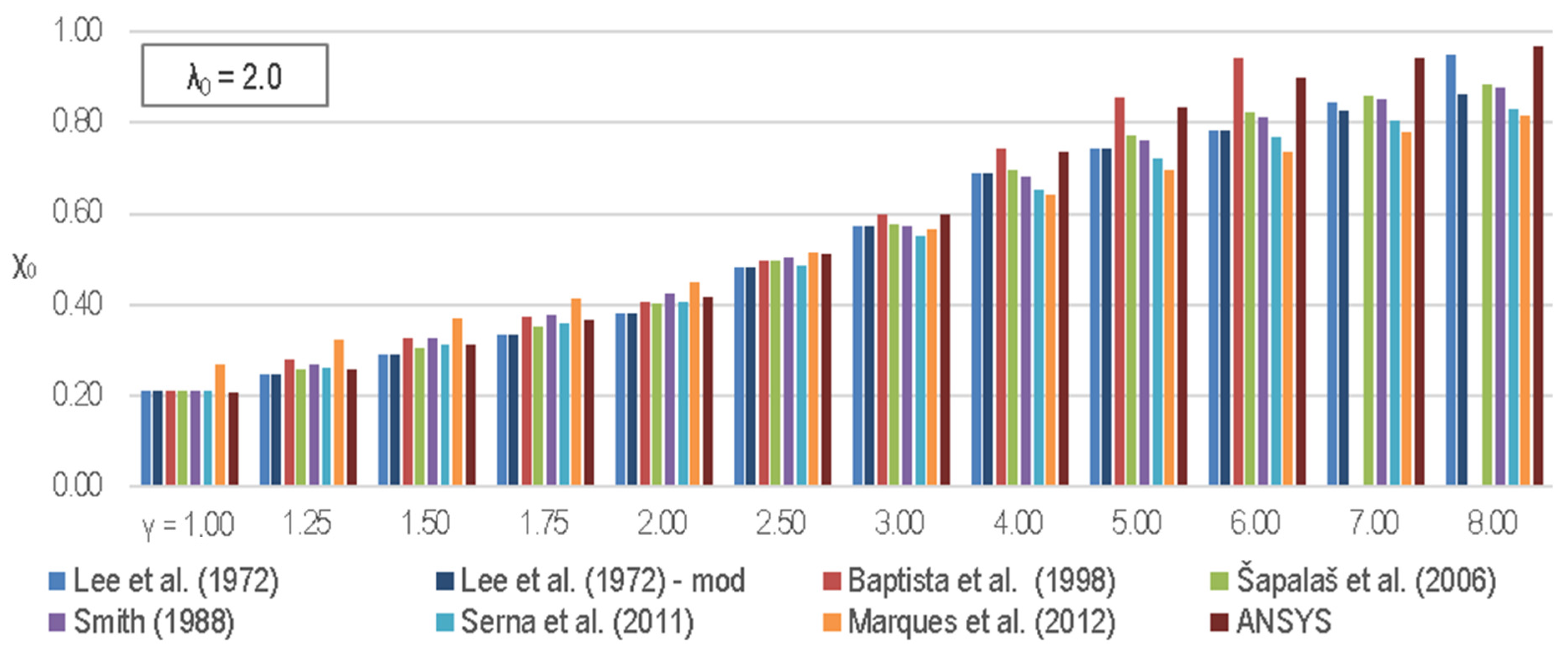
Analyzing Figure 15, which displays the normalized resistances versus the tapering ratios for λ₀ = 2.0, the resistances according to methodologies by Baptista et al. [21] and Lee et al. [8] deviated at higher tapering ratios. Excluding these, the resistances from the other methods were relatively close for all the tapering ratios. Therefore, the resistance from these deviating methodologies was excluded from the statistical analysis (

Table 8. Normalized resistance χ₀ depending on the tapering ratio γ—λ₀ = 2.0; HEB 300; S235.

λ0	2.0
γ	1.00	1.25	1.5	1.75	2.00	2.50	3.00	4.00	5.00	6.00	7.00	8.00
Lee et al. [8]—χL	0.21	0.25	0.29	0.33	0.38	0.48	0.57	0.69	0.74	0.78	0.85	0.95
Baptista et al. [21]—χB	0.21	0.28	0.33	0.37	0.41	0.50	0.60	0.74	0.86	0.94	-	-
Šapalaš et al. [32]—χŠ	0.21	0.26	0.30	0.35	0.40	0.50	0.58	0.70	0.77	0.82	0.86	0.89
Smith [44]—χS	0.21	0.27	0.33	0.38	0.42	0.50	0.57	0.68	0.76	0.81	0.85	0.88
Serna et al. [33]—χSe	0.21	0.26	0.31	0.36	0.41	0.49	0.55	0.65	0.72	0.77	0.80	0.83
Marques et al. [26]—χM	0.27	0.32	0.37	0.41	0.45	0.51	0.57	0.64	0.70	0.74	0.78	0.82
Lee et al. [8]—χL,mod	0.21	0.25	0.29	0.33	0.38	0.48	0.57	0.69	0.74	0.78	0.83	0.86
Mean value	0.22	0.27	0.32	0.37	0.41	0.50	0.57	0.67	0.74	0.79	0.82	0.85
Mean squared error	0.027	0.030	0.031	0.030	0.026	0.014	0.010	0.023	0.030	0.035	0.033	0.030
Coefficient of variation	0.122	0.112	0.099	0.082	0.062	0.027	0.017	0.034	0.041	0.044	0.040	0.036

). There was a more significant dispersion in the resistance results for the members with medium non-dimensional slenderness compared to those with low slenderness.

As shown in Table 8, as the tapering ratio increased, the dispersion of the results, measured by the coefficient of variation, decreased, reaching its lowest at γ = 3.0. Compared to a uniform member, the most substantial resistance increase per unit tapering ratio occurred at smaller tapering ratios, paralleling the trend with the members of low slenderness (

Table 9. Average normalized resistance χ_0,SV depending on the tapering ratio γ and the ratio of the resistance increase to the mass increase—λ₀ = 0.8; HEB 300; S235.

λ0	γ	χ0,SV	$\frac{{\mathit{\chi }}_0-{\mathit{\chi }}_0\left(\mathit{\gamma }=1\right)}{{\mathit{\chi }}_0\left(\mathit{\gamma }=1\right)}$	A [cm2]	$\frac{\mathit{A}-\mathit{A}\left(\mathit{\gamma }=1\right)}{\mathit{A}\left(\mathit{\gamma }=1\right)}$	$\frac{{\mathit{\chi }}_0-{\mathit{\chi }}_0\left(\mathit{\gamma }=1\right)/{\mathit{\chi }}_0\left(\mathit{\gamma }=1\right)}{\mathit{A}-\mathit{A}\left(\mathit{\gamma }=1\right)/\mathit{A}\left(\mathit{\gamma }=1\right)}$
1	2	3	4	5	6	4/6
0.8	1.00	0.22	0.00	142.82	0.00	-
	1.25	0.27	0.23	146.95	0.03	7.88
	1.50	0.32	0.45	151.07	0.06	7.76
	1.75	0.37	0.66	155.195	0.09	7.63
	2.00	0.41	0.87	159.32	0.12	7.50
	2.50	0.50	1.24	167.57	0.17	7.17
	3.00	0.57	1.56	175.82	0.23	6.77
	4.00	0.67	2.04	192.32	0.35	5.88
	5.00	0.74	2.34	208.82	0.46	5.06
	6.00	0.79	2.55	225.32	0.58	4.41
	7.00	0.82	2.72	241.82	0.69	3.93
	8.00	0.85	2.86	258.32	0.81	3.54

χ_0,SV—mean value of the normalized resistance; A—cross-sectional area at L/2.

). Furthermore, the tapering ratio’s impact on the resistance was considerably more significant in the members with a low slenderness. A member with γ = 8.0 offered 286% more resistance than a uniform one but has 81% more mass. Economically, the best resistance increase relative to the mass increase ratio was found in the members with a taper ratio of γ = 1.25. It was intriguing that for all the tapering ratios, the rise in the resistance substantially exceeded the mass increase relative to a uniform member, a phenomenon not witnessed with members of a low slenderness. However, this pattern aligned with the more significant influence of the tapering ratio on the buckling resistance identified for the members with a low slenderness.

Table 10. Normalized resistances compared to the normalized resistances, according to the methodology conceived by Marques et al. [24]—λ₀ = 2.0; HEB 300; S235.

γ	1.00	1.25	1.5	1.75	2.00	2.50	3.00	4.00	5.00	6.00	7.00	8.00
Marques et al. [26]—χM	0.27	0.32	0.37	0.41	0.45	0.51	0.57	0.64	0.70	0.74	0.78	0.82
χŠ/χM	0.78	0.79	0.82	0.85	0.90	0.97	1.02	1.08	1.11	1.12	1.10	1.09
χS/χM	0.78	0.83	0.88	0.92	0.94	0.98	1.01	1.06	1.09	1.10	1.09	1.08
χSe/χM	0.78	0.81	0.84	0.87	0.90	0.94	0.98	1.02	1.04	1.05	1.03	1.02
χL,mod/χM	0.78	0.76	0.78	0.81	0.85	0.94	1.01	1.07	1.07	1.06	1.06	1.06
Mean value	0.78	0.80	0.83	0.86	0.90	0.96	1.00	1.06	1.08	1.08	1.07	1.06
Coefficient of variation	0.003	0.037	0.052	0.052	0.042	0.021	0.019	0.027	0.029	0.031	0.030	0.028

shows the ratios of the calculated normalized buckling resistances using various methodologies and those according to the methodology by Marques et al. [26] for the varied taper ratios and a slenderness of λ₀ = 2.0. It was evident that all the methodologies predicted a lower resistance for the members up to a tapering ratio of γ = 3.0, while for the ratios above γ = 3.0, the reference methodology anticipated higher resistances. The resistance ratios were uniform across all the tapering ratios, as indicated by the maximum coefficient of variation of 0.085 for a member with a taper ratio of γ = 1.50.

The obtained normalized resistances for the members of a high slenderness, with λ₀ = 5.0, across the varied tapering ratios are presented in Figure 16. The results deviated significantly at larger taper ratios, particularly for the method proposed by Lee et al. [8]. Thus, the modified results, denoted as Lee et al.—mod, were used for the comparison and statistical calculations. The method proposed by Marques et al. [26] gave the smallest buckling resistance values, and as the tapering ratio increased, the results became more dispersed. With the increase in the tapering ratio, both the buckling resistance and the coefficient of variation increased (

Table 11. Normalized resistance χ₀ depending on the tapering ratio γ—λ₀ = 5.0; HEB 300; S235.

λ0	5.0
γ	1.00	2.50	3.00	4.00	5.00	6.00	7.00	8.00
Lee et al. [8]—χL	0.04	0.10	0.13	0.19	0.23	0.26	0.36	0.70
Baptista et al. [21]—χB	0.04	0.11	0.14	0.19	0.22	0.26	-	-
Šapalaš et al. [32]—χŠ	0.04	0.11	0.13	0.19	0.25	0.32	0.39	0.46
Smith [44]—χS	0.04	0.11	0.13	0.18	0.24	0.30	0.37	0.43
Serna et al. [33]—χSe	0.04	0.10	0.12	0.17	0.21	0.25	0.29	0.33
Marques et al. [26]—χM	0.05	0.11	0.13	0.16	0.20	0.23	0.24	0.27
Lee et al. [8]—χL,mod	0.04	0.10	0.13	0.19	0.23	0.26	0.33	0.40
Mean value	0.04	0.10	0.13	0.18	0.22	0.27	0.32	0.38
Mean squared error	0.005	0.004	0.004	0.012	0.023	0.038	0.059	0.078
Coefficient of variation	0.116	0.035	0.027	0.069	0.102	0.138	0.184	0.206

), with the latter being the smallest for the tapering ratio of γ = 3.0 (0.027) and the largest for γ = 8.0 (0.206). Discrepancies were most prominent for the method by Marques et al. [26], suggesting potential calibration issues with high tapering ratios and slenderness.

The tapering ratio’s impact on the resistance was most pronounced for the members with a high slenderness despite a smaller resistance range than those with a medium slenderness (

Table 12. Average normalized resistance χ_0,SV depending on the tapering ratio γ and the ratio of the resistance increase to the mass increase—λ₀ = 5.0; HEB 300; S235.

λ0	γ	χ0,SV	$\frac{{\mathit{\chi }}_0-{\mathit{\chi }}_0\left(\mathit{\gamma }=1\right)}{{\mathit{\chi }}_0\left(\mathit{\gamma }=1\right)}$	A [cm2]	$\frac{\mathit{A}-\mathit{A}\left(\mathit{\gamma }=1\right)}{\mathit{A}\left(\mathit{\gamma }=1\right)}$	$\frac{{\mathit{\chi }}_0-{\mathit{\chi }}_0\left(\mathit{\gamma }=1\right)/{\mathit{\chi }}_0\left(\mathit{\gamma }=1\right)}{\mathit{A}-\mathit{A}\left(\mathit{\gamma }=1\right)/\mathit{A}\left(\mathit{\gamma }=1\right)}$
1	2	3	4	5	6	4/6
0.8	1.00	0.04	0.00	142.82	0.00	-
	2.50	0.10	1.65	167.57	0.17	9.53
	3.00	0.13	2.25	175.82	0.23	9.75
	4.00	0.18	3.48	192.32	0.35	10.04
	5.00	0.22	4.68	208.82	0.46	10.13
	6.00	0.27	5.92	225.32	0.58	10.25
	7.00	0.32	7.18	241.82	0.69	10.36
	8.00	0.38	8.57	258.32	0.81	10.59

χ_0,SV—mean value of the normalized resistance; A—cross-sectional area at L/2.

). A member with the highest tapering ratio (γ = 8.0) displayed a resistance increase of 857% compared to a uniform member. In the members with a high slenderness, both the increase in the resistance per unit of the tapering ratio and the ratio of the resistance increase to the mass increase rose. Notably, a member with a tapering ratio of γ = 8.0 showed a resistance increase 10.59 times greater than its mass increase in relation to a uniform member.

Compared to Marques et al.’s reference method [26], the other methods predicted lower resistances up to a taper ratio of γ = 3.0 and higher (

Table 13. Normalized resistances compared to the normalized resistances, according to the methodology conceived by Marques et al. [24]—λ₀ = 5.0; HEB 300; S235.

γ	1.00	2.50	3.00	4.00	5.00	6.00	7.00	8.00
Marques et al. [26]—χM	0.05	0.11	0.13	0.16	0.20	0.23	0.24	0.27
χŠ/χM	0.79	0.97	1.04	1.17	1.29	1.40	1.61	1.70
χS/χM	0.79	0.98	1.02	1.12	1.23	1.33	1.53	1.62
χSe/χM	0.79	0.93	0.97	1.02	1.06	1.09	1.20	1.23
χL,mod/χM	0.79	0.92	1.02	1.15	1.16	1.16	1.35	1.49
Mean value	0.79	0.95	1.01	1.11	1.18	1.24	1.42	1.51
Coefficient of variation	0.0004	0.0302	0.0307	0.0571	0.0815	0.1143	0.1277	0.1356

). The deviation from the reference increased with the tapering ratio, with the slightest deviations for the methodology by Serna et al. [33].

4.3. Evaluation of the Applicability of a Specific Methodology

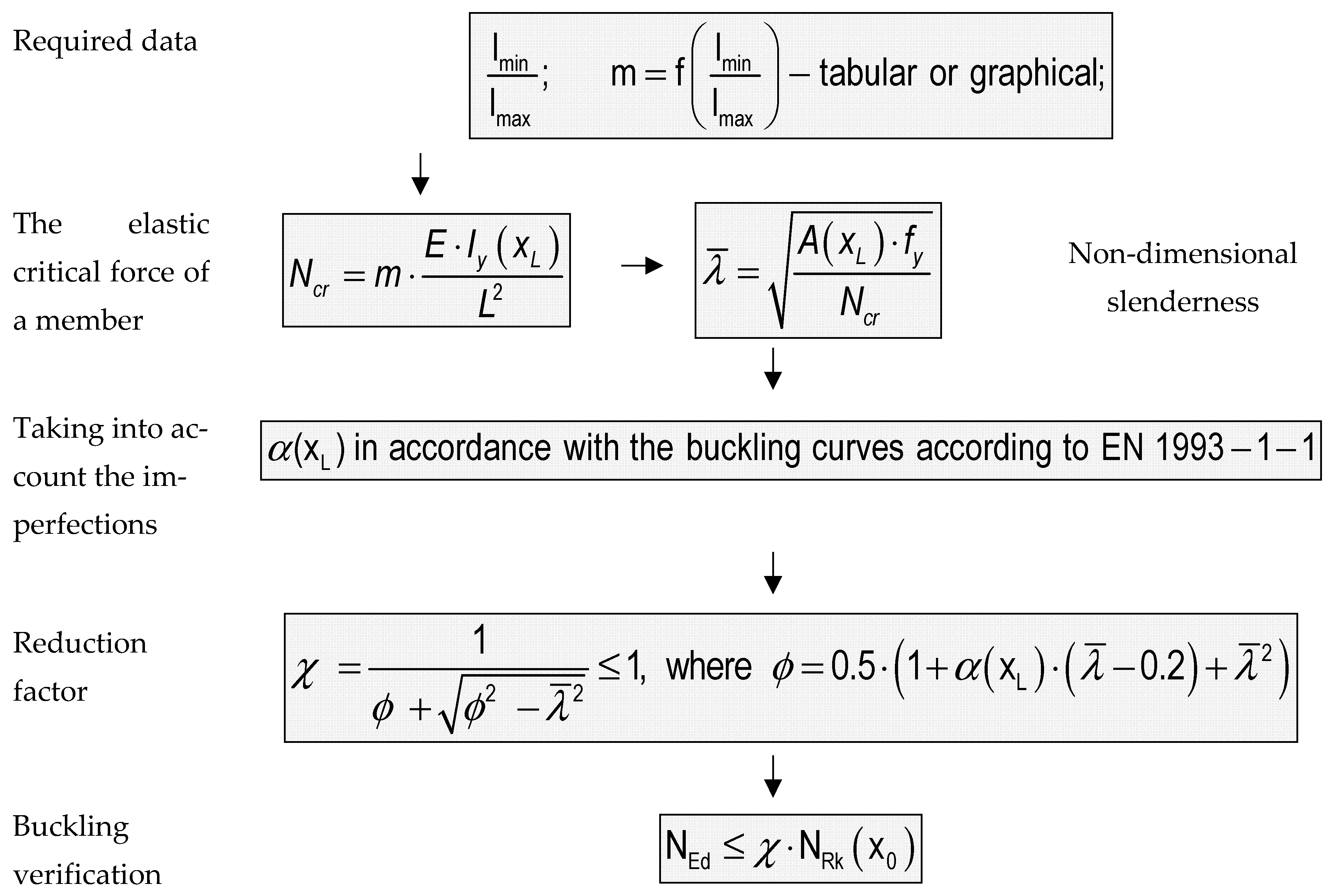
Assessing the suitability of specific methodologies considered their application potential within the existing regulatory framework (computation sequence per EN 1993-1-1 [22]). This assessment factored in the discrepancies in the computation results compared to the benchmark methodology (Marques et al. [26]). The idea revolved around the balance between introducing new variables required for calculating a member’s resistance and maintaining the simplicity and intelligibility of the computational process for engineers. Increased complexity can lead to a higher potential for errors and reduced clarity of the process.

Each methodology introduced a unique set of variables for calculating the buckling resistance for non-uniform members, as seen in Section 2’s calculation procedures. For example, the method by Lee et al. [8] included just two new variables, the taper ratio γ and the length change factor g, then proceeded according to the standard EN 1993-1-1 methodology. The other methods, like those proposed by Baptista et al. [21] and Šapalas et al. [32], introduced three or four new variables. Along with the Lee et al. [27] method, these were relatively simple, requiring minimal additional computations. Contrarily, the methodologies proposed by Serna et al. [33] and Marques et al. [26] were complex, requiring many new variables and computational steps, including numerical buckling simulations for each case. For instance, the Serna et al. [33] calculation procedure introduced 12 new variables, and after their determination, the conventional computation for a uniform member began. Marques et al. [26] introduced nine new variables, one of which needed to be determined by a numerical buckling simulation, increasing the complexity and time required for each case. A summary of the required additional variables for the non-uniform member calculations, compared to the uniform element calculations, is provided in

Table 14. Number of additional calculations needed to determine the resistance of a non-uniform member compared to the calculation of a uniform member, according to EN 1993-1-1.

	Lee et al. [8]	Baptista et al. [21]	Šapalaš et al. [32]	Smith [44]	Serna et al. [33]	Marques et al. [26]	Lee et al. [8]—mod
Number of new variables n	2	3	4	3	12	9 (12)	2

.

In order to evaluate the deviation of the results of each methodology from the reference one (Marques et al. [26]), all the possible combinations of variables in the parametric analysis were considered. The ratios of the normalized resistances of each methodology and the reference one for the same non-dimensional slenderness and tapering ratio were examined (

Table 15. Average values of the ratios of the normalized resistance, according to the used calculation methodologies, and the normalized resistance, according to the methodology proposed by Marques et al. [26].

	γ = 1.00–6.00
	Marques et al. [26]/Marques et al. [26]	Lee et al. [8]/ Marques et al. [26]	Baptista et al. [21]/Marques et al. [26]	Šapalaš et al. [32]/Marques et al. [26]	Smith [44]/Marques et al. [26]	Serna et al. [33]/Marques et al. [26]	Lee et al. [8]—mod./Marques et al. [26]
	χM/χM	χL/χM	χB/χM	χŠ/χM	χS/χM	χSe/χM	χL,mod/χM
Mean value	1.0	1.00	1.06	1.04	1.04	0.98	1.00
Coefficient of variation	0.0	0.13	0.12	0.17	0.13	0.09	0.13
	γ = 1.00–8.00
	Marques et al. [26]/Marques et al. [26]	Lee et al. [8]/Marques et al. [26]	Baptista et al. [21]/Marques et al. [26]	Šapalaš et al. [32]/Marques et al. [26]	Smith [44]/Marques et al. [26]	Serna et al. [33]/Marques et al. [26]	Lee et al. [8]—mod./Marques et al. [26]
	χM/χM	χL/χM	χB/χM	χŠ/χM	χS/χM	χSe/χM	χL,mod/χM
Mean value	1.0	1.17	1.06	1.13	1.11	1.01	1.06
Coefficient of variation	0.0	0.46	0.12	0.23	0.20	0.11	0.17

). In the most commonly used taper ratio range, γ = 1.0–γ = 6.0, the most minor deviation from the reference methodology was shown by the methodologies of Lee et al. [8] and Serna et al. [33]. In order to include a specific parameter in the assessment of its applicability, its importance must be assigned in the context of the purpose of the calculation and engineering aspirations. Following the goal for the results to be as close as possible to those of the reference methodology, the average value of the ratio of a particular methodology represented 50% of the applicability rating, with an additional 25% deviation (coefficient of variation). The remaining 25% of the rating represented the number of additional variables compared to calculating a uniform member. In order to compare the results, each parameter was assigned the same number of points, and then the importance of the parameter was included by weighting the number of points. The ranking of the methodologies’ applicability was obtained by ranking the number of points.

The evaluation process was undertaken by assigning scores to each criterion. For the average value, a score of 10 was given if the result was precisely 1.0, while a result of either 1.25 or 0.75 received zero points. This implied that any divergence greater than 0.25 was undesirable and received no points. Points for the results between these values were allocated using linear interpolation. Regarding the variance of the results, a correlation coefficient of 0.0 yielded 10 points, while a value of 0.25 received none, with all the other scores determined via linear interpolation. The points associated with the count of the additional variables were distributed so that having only two extra variables compared to the uniform element calculation yielded 10 points, with every additional variable reducing the score by 1. If the methodology required computing 12 additional variables, it was given zero points. According to this system,

Table 16. Assessment and ranking of the applicability of the observed calculation methodologies for non-uniform members, depending on the examined area of the tapering ratio γ.

		γ = 1.00–6.00
		Marques et al. [26]	Lee et al. [8]	Baptista et al. [21]	Šapalaš et al. [32]	Smith [44]	Serna et al. [33]	Lee et al. [8] —mod.
Points	Mean value	10.00	9.84	7.68	8.23	8.34	9.31	9.84
	Coefficient of variation	10.00	4.72	5.21	3.30	4.65	6.49	4.72
	Number of variables	0.00	10.00	9.00	8.00	9.00	0.00	10.00
Total (Weighted)		7.50	8.60	7.39	6.94	7.58	6.28	8.60
Rank		3.	1.	4.	5.	2.	6.	1.
		γ = 1.00–8.00
		Marques et al. [26]	Lee et al. [8]	Baptista et al. [21]	Šapalaš et al. [32]	Smith [44]	Serna et al. [33]	Lee et al. [8] —mod.
Points	Mean value	10.00	3.25		4.95	5.51	9.40	7.79
	Coefficient of variation	10.00	0.00		0.74	2.11	5.80	3.02
	Number of variables	0.00	10.00		8.00	9.00	0.00	10.00
Total (Weighted)		7.50	4.13		4.66	5.53	6.15	7.15
Rank		1.	6.		5.	4.	3.	2.

presents each methodology’s individual and total weighted scores. Based on the points earned for the most realistic tapering ratios, γ = 1.0–γ =6.0, the method developed by Lee et al. [8] scored the highest. This was mainly due to the simplicity of this method while maintaining a reasonable deviation from the reference methodology. When the range of the observed tapering ratios was extended to γ = 8.0, the reference methodology took the top spot, with the adapted version of the methodology suggested by Lee et al. [8] coming in second. This aligned with the philosophy of the European standards, which permit more straightforward methods for less complex problems (γ = 1.0–γ = 6.0), accepting a tolerable loss of “precision”, whereas for more intricate problems (γ = 6.0–γ = 8.0) they mandate more detailed analyses.

5. Conclusions

The presented research highlights the complexity of calculating the buckling resistance for tapered members. The findings can guide structural engineers in selecting the appropriate calculation methodologies for specific scenarios and help bridge the existing gap in design standards. Future research should be focused on conducting experiments to validate these findings further and refine these methodologies.

In conclusion, our study on the buckling resistance of members with varying cross-sections revealed several significant findings and implications.

• Regulatory gap: Modern standards, such as EN 1993 and AISC 360, lack clear guidelines for calculating the buckling resistance of members with variable cross-sections. This regulatory gap often causes engineers to make conservative assumptions, resulting in suboptimal designs.
• Relevance of the issue: Recent research in well-cited journals highlight the continued relevance and importance of addressing the challenges associated with variable cross-section members.
• Calculation proposals: Several calculation methodologies have been proposed for non-uniform elements, each with unique strengths and limitations. These methodologies include the works by Lee et al. [8], Baptista et al. [21], Šapalas et al. [32], Smith [44], Serna et al. [33], and Marques et al. [26].
• Discrepancies across the methodologies: Through an extensive parametric analysis, we observed discrepancies in the calculated buckling resistance of non-uniform members, especially with varying tapering ratios and slenderness values. These variations were particularly pronounced for medium-slenderness members and decreased as the tapering ratio increased.
• Optimal tapering ratios: The optimal tapering ratio for the resistance-to-mass gain differed depending on the slenderness category. For low-slenderness members, ratios below γ = 3.0 were economically optimal, while for medium-slenderness members, γ = 1.25 provided the best balance between the resistance and mass gain. High-slenderness members saw a more significant increase in the resistance with the tapering ratio.
• Comparison with the benchmark method: Compared to the benchmark method (Marques et al. [26]), various calculation methods projected lower resistances for low to medium-slenderness members. However, beyond a tapering ratio of γ = 3.0, they predicted higher resistances than the benchmark. The largest discrepancies from the mean occurred with high tapering ratios and slenderness values, indicating potential calibration issues for these scenarios.
• Comparison with the numerical models: Our study indicated that, when compared to the ANSYS numerical models, some calculation methods tended to predict lower reduction factors and buckling resistances, especially for a lower slenderness, while Baptista et al.’s [21] method tended to overestimate these values in that slenderness range.
• Applicability assessment: A scoring system was applied to evaluate the applicability of the methodologies. Lee et al.’s method scored the highest for the tapering ratios of γ = 1.0–6.0 due to its simplicity and proximity to the benchmark method (Marques et al. [26]). Extending the tapering range to γ = 8.0, Marques et al.’s [26] method became the most applicable. This aligned with the European norms, which prefer straightforward methods for less complex scenarios (γ = 1.0–γ = 6.0) but require detailed analyses for more complex problems (γ = 6.0–γ = 8.0).

References

1. Structural Stability Research Council. Guide to Stability Design Criteria for Metal Structures, 6th ed.; Ziemian, D.R., Ed.; John Wiley & Sons, Inc.: New York, NY, USA, 2010; p. 1117. [Google Scholar]
2. Timoshenko, P.S.; Gere, M.J. Theory of Elastic Stability, 2nd ed.; McGraw-Hill: Mineola, NY, USA, 1961. [Google Scholar]
3. Timoshenko, P.S. Theory of Elastic Stability; McGraw-Hill: New York, NY, USA, 1936. [Google Scholar]
4. Newmark, N.M. Numerical Procedure for Computing Deflections, Moments, and Buckling Loads. Trans. Am. Soc. Civ. Eng 1943, 108, 1161–1188. [Google Scholar] [CrossRef]
5. Butler, D.J. Elastic Buckling Tests on Laterally and Torsionally Braced Tapered I-Beams. Weld. J. 1966, 44, 41–48. [Google Scholar]
6. Butler, D.J.; Anderson, G.C. The elastic buckling of tapered beam-columns. Weld. J. 1963, 42, 29–36. [Google Scholar]
7. Prawel, S.P.; Morrell, M.L.; Lee, G.C. Bending and buckling strength of tapered structural members. Weld. J. 1974, 53, 75–84. [Google Scholar]
8. Lee, G.C.; Morrell, M.L.; Ketter, R.L. Design of Tapered Members; Welding Research Council Bulletin: New York, NY, USA, 1972; pp. 1–32. [Google Scholar]
9. American Institute of Steel Construction (AISC). Specification for the Design, Fabrication and Erection of Structural Steel for Buildings; AISC: Chicago, IL, USA, 1978. [Google Scholar]
10. Hirt, M.A.; Crisinel, M. Charpentes Métalliques: Conception et Dimensionnement des Halles et Bâtiments; PPUR presses polytechniques: Vaud, Switzerland, 2005; Volume 11. [Google Scholar]
11. Salter, J.B.; Anderson, D.; May, I.M. Tests on Tapered Steel Columns. Struct. Eng. 1980, 58, 189–193. [Google Scholar]
12. Shiomi, H.; Kurata, M. Strength Formula for Tapered Beam-Columns. J. Struct. Eng. 1984, 110, 1630–1643. [Google Scholar] [CrossRef]
13. Shiomi, H.; Nishikawa, S.-I.; Kurata, M. An Experimental Study on Ultimate Strength of Steel Tapered Beam-Columns. Mem. Chbu Inst. Technol. A 1983, 19, 55–66. [Google Scholar]
14. Forest, R.; Murray, T. Rigid Frame Studies, Full Scale Frame Tests. In Research Report No. FSEL/STAR 82-01; School of Civil Engineering and Environmental Science: Norman, OK, USA, 1982. [Google Scholar]
15. Lee, G.C.; Ketter, R.L.; Hsu, T.L. The Design of Single Story Rigid Frames; Metal Building Manufacturers Association: Cleveland, OH, USA, 1981. [Google Scholar]
16. White, D.W.; Kim, Y.D. A Prototype Application of the AISC (2005) Stability Analysis and Design Provisions to Metal Building Structural Systems; Georgia Institute of Technology: Atlanta, GA, USA, 2006. [Google Scholar]
17. American Institute of Steel Construction (AISC). AISC 360-05, Specification for Structural Steel Buildings; AISC: Chicago, IL, USA, 2005. [Google Scholar]
18. Ronagh, H.R.; Bradford, M.A.; Attard, M.M. Nonlinear analysis of thin-walled members of variable cross-section. Part I: Theory. Comput. Struct. 2000, 77, 285–299. [Google Scholar] [CrossRef]
19. Ronagh, H.R.; Bradford, M.A.; Attard, M.M. Nonlinear analysis of thin-walled members of variable cross-section. Part II: Application. Comput. Struct. 2000, 77, 301–313. [Google Scholar] [CrossRef]
20. Boissonnade, N.; Maquoi, R.A. Geometrically and Materially Non-linear 3-D Beam Finite Element for the Analysis of Tapered Steel Members. Steel Struct. 2005, 5, 413–419. [Google Scholar]
21. Baptista, A.M.; Muzeau, J.P. Design of tapered compression members according to Eurocode 3. J. Constr. Steel Res. 1998, 46, 146–148. [Google Scholar] [CrossRef]
22. European Committee for Standardization (CEN). EN 1993-1-1, Eurocode 3: Design of Steel Structures—Part 1-1: General Rules and Rules for Buildings; CEN: Brussels, Belgium, 2005. [Google Scholar]
23. Ermopoulos, J.C. Equivalent buckling length of non-uniform members. J. Constr. Steel Res. 1997, 42, 141–158. [Google Scholar] [CrossRef]
24. Ermopoulos, J.C. Buckling length of non-uniform members under stepped axial loads. Comput. Struct. 1999, 73, 573–582. [Google Scholar] [CrossRef]
25. Simões da Silva, L.; Rebelo, C.; Marques, L. Application of the general method for the evaluation of the stability resistance of non-uniform members. In Proceedings of the Sixth International Conference on Advances in Steel Structures-ICASS, Hong Kong, China, 16–19 December 2009. [Google Scholar]
26. Marques, L.; Taras, A.; da Silva, L.S.; Greiner, R.; Rebelo, C. Development of a consistent buckling design procedure for tapered columns. J. Constr. Steel Res. 2012, 72, 61–74. [Google Scholar] [CrossRef]
27. Quan, C.; Kucukler, M.; Gardner, L. Design of web-tapered steel I-section members by second-order inelastic analysis with strain limits. Eng. Struct. 2020, 224, 111242. [Google Scholar] [CrossRef]
28. Bai, R.; Liu, S.W.; Liu, Y.P.; Chan, S.L. Direct analysis of tapered-I-section columns by one-element-per-member models with the appropriate geometric-imperfections. Eng. Struct. 2019, 183, 907–921. [Google Scholar] [CrossRef]
29. Abdelrahman, A.H.A.; Lotfy, S.; Liu, S.-W. Generalized line-element formulations for geometrically nonlinear analysis of nonsymmetric tapered steel members with warping and Wagner effects. Eng. Struct. 2022, 273, 115052. [Google Scholar] [CrossRef]
30. Chen, W.F.; Liu, Y.P.; Du, Z.L.; Bai, R.; Chan, S.L. A consistent tapered beam-column element allowing for different variations and initial imperfections. Structures 2021, 33, 3443–3460. [Google Scholar] [CrossRef]
31. Kucukler, M.; Gardner, L. Design of laterally restrained web-tapered steel structures through a stiffness reduction method. J. Constr. Steel Res. 2018, 141, 63–76. [Google Scholar] [CrossRef]
32. Šapalas, V.; Samofalov, M.; Šaraškinas, V. Fem stability analysis of tapered beam-columns. J. Civ. Eng. Manag. 2005, 11, 211–216. [Google Scholar] [CrossRef]
33. Serna, M.A.; Ibáñez, J.R.; López, A. Elastic flexural buckling of non-uniform members: Closed-form expression and equivalent load approach. J. Constr. Steel Res. 2011, 67, 1078–1085. [Google Scholar] [CrossRef]
34. Nguyen, T.-H.; Tran, N.-L.; Nguyen, D.-D. Prediction of Critical Buckling Load of Web Tapered I-Section Steel Columns Using Artificial Neural Networks. Int. J. Steel Struct. 2021, 21, 1159–1181. [Google Scholar] [CrossRef]
35. Ibrahim, S.M. Effective buckling length of frames with tapered columns and partially tapered beams. J. Constr. Steel Res. 2021, 187, 106993. [Google Scholar] [CrossRef]
36. Mahini, M.R. An Efficient K-Factor Formula for Stability Evaluation of Steel Frames with Web-Tapered Members. Iran. J. Sci. Technol. Trans. Civ. Eng. 2023, 47, 1673–1687. [Google Scholar] [CrossRef]
37. Zhu, R.; Liu, Y.; Bojja, N.; Qin, Z.; Chu, F. Vibration attenuation of rotating disks via acoustic black holes. Int. J. Mech. Sci. 2023, 242, 108025. [Google Scholar] [CrossRef]
38. Gao, W.; Qin, Z.; Chu, F. Broadband vibration suppression of rainbow metamaterials with acoustic black hole. Int. J. Mech. Sci. 2022, 228, 107485. [Google Scholar] [CrossRef]
39. Zhang, L.; Tang, X.; Qin, Z.; Chu, F. Vibro-impact energy harvester for low frequency vibration enhanced by acoustic black hole. Appl. Phys. Lett. 2022, 121, 013902. [Google Scholar] [CrossRef]
40. Nguyen, H.N.; Tan, T.C.; Luat, D.T.; Phan, V.D.; Thom, D.V.; Minh, P.V. Research on the Buckling Behavior of Functionally Graded Plates with Stiffeners Based on the Third-Order Shear Deformation Theory. Materials 2019, 12, 1262. [Google Scholar] [CrossRef]
41. Nguyen Thai, D.; Minh, P.V.; Phan Hoang, C.; Ta Duc, T.; Nguyen Thi Cam, N.; Nguyen Thi, D. Bending of Symmetric Sandwich FGM Beams with Shear Connectors. Math. Probl. Eng. 2021, 2021, 7596300. [Google Scholar] [CrossRef]
42. Phung, V.M.; Ta, D.T.; Tran, V.K. Static bending analysis of symmetrical three-layer fgm beam with shear connectors under static load. J. Sci. Tech. 2021, 15, 3. [Google Scholar] [CrossRef]
43. Phung, M.V.; Nguyen, D.T.; Doan, L.T.; Nguyen, D.V.; Duong, T.V. Numerical Investigation on Static Bending and Free Vibration Responses of Two-Layer Variable Thickness Plates with Shear Connectors. Iran. J. Sci. Technol. Trans. Mech. Eng. 2022, 46, 1047–1065. [Google Scholar] [CrossRef]
44. Smith, W.G. Analytic solutions for tapered column buckling. Comput. Struct. 1988, 28, 677–681. [Google Scholar] [CrossRef]
45. Kaehler, R.C.; White, D.W.; Kim, Y.D. Frame Design Using Web-Tapered Members; American Institute of Steel Construction: Chicago, IL, USA, 2011. [Google Scholar]
Figure 1. Tapered steel column.
Applsci 13 11498 g001
Figure 2. The process of integrating the buckling calculation into EN 1993-1-1, according to the methodology proposed by Lee et al. [27].
Applsci 13 11498 g002
Figure 3. The process of integrating the buckling calculation into EN 1993-1-1, according to the methodology proposed by Baptista et al. [19].
Applsci 13 11498 g003
Figure 4. Coefficients k for a non-uniform element doubly hinged and loaded by bending around the strong axis [21].
Applsci 13 11498 g004
Figure 5. The process of integrating the buckling calculation into EN 1993-1-1, according to the methodology proposed by Šapalas et al. [25].
Applsci 13 11498 g005
Figure 6. The process of integrating the buckling calculation into EN 1993-1-1, according to the methodology proposed by Smith [28].
Applsci 13 11498 g006
Figure 7. The process of integrating the buckling calculation into EN 1993-1-1, according to the methodology proposed by Serna et al. [26].
Applsci 13 11498 g007
Figure 8. The process of integrating the buckling calculation into EN 1993-1-1, according to the methodology proposed by Marques et al. [24].
Applsci 13 11498 g008aApplsci 13 11498 g008b
Figure 9. ANSYS project schematic (a) and a buckled tapered steel column (b).
Applsci 13 11498 g009
Figure 10. Functional relationship between the coefficient k and the slenderness prescribed by the methodology [19], according to Equations (15)–(21).
Applsci 13 11498 g010
Figure 11. The relationship between the normalized resistance (χ0) and non-dimensional slenderness of the smallest cross-section (λ0) for the various calculation methods [8,21,22,26,32,33,44]—tapering ratio (a) γ = 1.0 and (b) 1.25.
Applsci 13 11498 g011
Figure 12. The relationship between the normalized resistance (χ0) and non-dimensional slenderness of the smallest cross-section (λ0) for the various calculation methods [8,21,22,26,32,33,44]—tapering ratio (a) γ = 1.50 and (b) 2.0.
Applsci 13 11498 g012
Figure 13. The relationship between the normalized resistance (χ0) and non-dimensional slenderness of the smallest cross-section (λ0) for the various calculation methods [8,21,22,26,32,33,44]—tapering ratio (a) γ = 4.0 and (b) 6.0.
Applsci 13 11498 g013
Figure 14. Normalized resistances (χ0) for the varied tapering ratios (γ) and a non-dimensional slenderness of λ0 = 0.8 - [8,21,22,26,32,33,44].
Applsci 13 11498 g014
Figure 15. Normalized resistances (χ0) for the varied tapering ratios (γ) and a non-dimensional slenderness of λ0 = 2.0—[8,21,22,26,32,33,44].
Applsci 13 11498 g015
Figure 16. Normalized resistances (χ0) for the varied tapering ratios (γ) and a non-dimensional slenderness of λ0 = 5.0—[8,21,22,26,32,33,44].
Applsci 13 11498 g016