FPGA Implementation of a Real-Time Edge Detection System Based on an Improved Canny Algorithm

Abstract

Canny edge detection is one of the most widely used edge detection algorithms due to its superior performance. However, it is a complex, time-consuming process and has a high hardware cost. To overcome these issues, an improved Canny algorithm is proposed in this paper. It uses the Sobel operator and approximation methods to calculate the gradient magnitude and direction for replacing complex operations with reduced hardware costs. Otsu’s algorithm is introduced to adaptively determine the image threshold. However, Otsu’s algorithm has division operations, and the division operation is complex and has low efficiency and slow speed. We introduce a logarithmic unit to turn the division into a subtraction operation that is easy to implement by hardware but does not affect the selection of the threshold. Experimental results show that the system can detect the edge of the image well without adjusting the threshold value when the external environment changes and requires only 1.231 ms to detect the edges of the 512 × 512 image when clocked at 50 MHz. Compared with existing FPGA implementations, our implementation uses the least amount of logical resources. Thus, it is more suitable for platforms that have limited logical resources.

1. Introduction

Image edge detection has important applications in many fields, such as medical imaging, geological exploration, satellite remote sensing, aerospace, transportation, and computer vision.

Many researchers have developed various edge detection approaches [1,2,3,4,5]. Edge detection approaches include the Robert detector [1], the Prewitt detector [2], the Sobel detector [3], the Laplace of Gaussian detector [4], and the Canny edge detector [5]. Among the existing edge detection algorithms, the Canny edge detection algorithm has been a standard for many years and has the best performance. However, the Canny edge detection algorithm is a complex, time-consuming process, and the traditional implementations of the algorithm use the same fixed pair of high and low threshold values for all input images. When the external environment, such as light, changes, the image to be detected will also change, and the threshold value needs to be adjusted. These shortcomings seriously affect the real-time performance, adaptive ability, and flexibility of the system. Therefore, a direct implementation of the Canny algorithm cannot be employed in real-time applications.

To solve these issues, researchers have proposed various techniques. One of these is the hardware implementation of the Canny edge detection algorithm based on a field programmable gate array (FPGA). Several works [6,7,8,9] have dealt with FPGA-based Canny edge detection algorithms for real-time applications. All of them reduce the complexity of the Canny edge detection algorithm to a certain extent and propose their solutions for threshold selection. In the existing hardware implementations, the threshold is usually obtained in two ways: fixed threshold and adaptive threshold. Using a fixed threshold can reduce the complexity of the algorithm, but it degrades the performance, as presented in [6]. The adaptive threshold based on the frame structure proposed in [7] calculates the threshold using the gradient histogram of the entire picture, which improves performance but increases latency. The determination of the appropriate threshold with minimal latency and computational cost is an important issue in the Canny edge detection technique. To address this issue, [8,9] introduces the distributed Canny edge detection technique, which has a low latency, high throughput, and resilient threshold computation approach. This method divides an image into several blocks and then uses the Canny edge detection algorithm for each block in parallel to reduce latency. The block-based technique computes low and high thresholds depending on the local features of each block, which aids in suppressing excessive edges in the smooth zone while preserving significant edges in the high-detailed region. Although the block-based Canny edge detection algorithm is more efficient than the frame-based Canny edge detection algorithm, the parallel implementation requires more resources and increases the computational complexity.

Another set of works [10,11,12] focuses on translating the Deriche filter generated from Canny’s criteria onto ASIC-based platforms. A 256 × 256 picture edge is discovered in 6 s using a Canny-Deriche filter network with four transputers [10], resulting in high latency. The implementation of the Canny-Deriche filter in [10] was improved in [11], which processes 25 frames/s at 33 MHz and uses off-chip SRAM memories with Last-In-First-Out (LIFO) stacks, which increases the area overhead compared to [10]. Ref. [12] proposes a novel structure of the Canny-Deriche filter to minimize memory space and calculation cost. However, processing time grows with picture size, and the number of clock cycles per pixel implementation varies with image size.

The recently developed general-purpose graphics processing unit (GPGPU) [13,14] provides a parallel computing platform for image processing applications. [15,16,17] investigates the implementation of Canny edge detection using GPGPU. The implementation performs poorly since it employs fixed high and low threshold settings for all pictures, but it performs better in terms of timing than all other implementations.

In this paper, an improved Canny edge detection algorithm is proposed with adequate accuracy, reduced computational complexity, and self-adaptive threshold calculation. We calculate the threshold using Otsu’s algorithm [18]. Several works have dealt with the FPGA-based Otsu’s algorithm for threshold calculation [19,20]. The approximate method and logarithm operation are introduced to reduce the complexity of computation. Our contributions in terms of the proposed design strategy are given below.

• Computation of the gradient magnitude and orientation using the approximate method.
• Using Otsu’s algorithm for adaptive threshold calculation.
• The design of a 32-bit logarithmic arithmetic unit to reduce the complexity of Otsu’s algorithm.

2. Proposed Design Strategy

2.1. Conventional Canny Edge Detection Algorithm

Canny developed an approach to derive an optimal edge detector to deal with step edges corrupted by white Gaussian noise. Figure 1 summarizes the original Canny edge detection algorithm [5] for an input image of size $M\times M$ with n bits each. It consists of the following steps:

(1)

Calculate the horizontal gradient G_x and vertical gradient G_y at each pixel location by convolving with gradient masks.

(2)

Compute the gradient magnitude G and direction θ_G at each pixel location.

(3)

Non maximum suppression (NMS): Convert blurred edges of the image into sharp edges and suppress minima (preserving local maxima) in the gradient image.

(4)

Computation of threshold: Potential edges are determined by high and low thresholds and are calculated based on the gradient magnitude histogram of the whole image.

(5)

Hysteresis thresholding: Creates a continuous edge map by comparing the values of the gradient magnitude of each pixel with low and high threshold values. This removes edge pixels caused by noise and illumination variation.

2.2. Improved Canny Edge Detection Algorithm

In all hardware implementations of the Canny edge detection algorithm, the method of selecting the threshold can be roughly divided into two types, namely, fixed and adaptive thresholds. The adoption of a fixed threshold will undoubtedly reduce algorithm complexity and hardware resource consumption. However, when the object to be detected changes or the external environment of the detected object changes, such as light, the threshold needs to be reset. This obviously cannot meet the requirements of real-time performance. In contrast, an adaptive threshold is a good solution to the above problems. In this section, we introduced three approaches to improve the Canny edge detection algorithm for hardware implementation, namely, Otsu’s algorithm, which is used to automatically select the threshold, low complexity gradient magnitude and direction calculation method, and logarithmic approximation, which is used to reduce the complexity of Otsu’s algorithm. Figure 2 shows an overview of the improved Canny edge detection design strategy. A detailed description of the proposed Canny edge detection algorithm is given below.

2.2.1. Gradient Computation Based on the Sobel Operator

Here, we use the Sobel operator [21,22] as a gradient mask. There is significant motivation for the employment of the Sobel operator rather than other operators used in [4,23] because it combines differentiation and Gaussian smoothing. More weight is allocated to pixel intensities around edges. Figure 3 shows the 3 × 3 sub-window of an image and Sobel operator kernels in the horizontal (x) and vertical (y) directions. The gradients in the x- and y-direction denoted by $f_x\left(x,y\right)$ and $f_y\left(x,y\right)$ are computed using Equations (1) and (2).

$$\begin{array}{c}{f}_x\left(x,y\right)=\left(p_2-p_0\right)+2\left(p_5-p_3\right)+\left(p_8-p_6\right)\end{array}$$

(1)

$$\begin{array}{c}{f}_y\left(x,y\right)=\left(p_6-p_0\right)+2\left(p_7-p_1\right)+\left(p_8-p_2\right)\end{array}$$

(2)

Before computing $f_x\left(x,y\right)$ and $f_y\left(x,y\right)$, we need to obtain the corresponding pixels. This is done by the Line Buffer. Figure 4 shows the architecture of the Line Buffer. Here we use two first-in-first-out (FIFO) modules to cache the first two rows.

After obtaining the corresponding pixels, the computation of $f_x\left(x,y\right)$ and $f_y\left(x,y\right)$ is started. Figure 5 shows the architecture to calculate $f_x\left(x,y\right)$. The architecture to calculate $f_y\left(x,y\right)$ is similar, and only the corresponding pixel values that are involved in the computation are different. In this part, the computation values of $f_x\left(x,y\right)$ and $f_y\left(x,y\right)$ are signed numbers, and their most significant bits (MSBs) determine whether their values are positive or negative.

2.2.2. Low Complexity Gradient Magnitude and Direction Calculation

The magnitude of the pixel defines the strength of the edge at a particular pixel. The orientation of a pixel defines the direction of the edge at a particular pixel. The gradient magnitude and direction calculations of a single pixel are given in Equations (3) and (4)

$$\begin{array}{c}mag\left(x,y\right)=\sqrt{f_x{\left(x,y\right)}^2+f_y{\left(x,y\right)}^2}\end{array}$$

(3)

$$\begin{array}{c}\theta \left(x,y\right)=\mathrm{a}\mathrm{r}\mathrm{c}\mathrm{t}\mathrm{a}\mathrm{n}\left(\frac{f_y\left(x,y\right)}{f_x\left(x,y\right)}\right)\end{array}$$

(4)

The hardware cost of implementing Equations (3) and (4) is high. For Equation (3), we use the addition of the absolute values of $f_x\left(x,y\right)$ and $f_y\left(x,y\right)$, which are presented in [21,22], to find the gradient magnitude mag (x, y). Equation (3) can be rewritten as

$$\begin{array}{c}mag\left(x,y\right)=\left|f_x\left(x,y\right)\right|+\left|f_y\left(x,y\right)\right|\end{array}$$

(5)

For Equation (4), the coordinate rotation digital computer (CORDIC) module suggested in [24,25] is used to calculate the value of θ(x,y). The downside of the CORDIC module is that many iterations are required to achieve acceptable accuracy, which leads to the utilization of more hardware. In this part, the shift-based orientation method [9] is adopted. The orientations are spaced uniformly and are divided into eight zones, as shown in Figure 6. The approximated values of $tan\theta \left(x,y\right)$ based on shift operations are listed in

Table 1. Shift-based tangent value computation.

Tangent	Approximate Value	Tangent	Approximate Value
tan 0°	0	tan 112.5°	−tan 67.5°
tan 22.5°	$2^{-2}+2^{-3}+2^{-5}+2^{-7}$	tan 135°	−tan 45°
tan 45°	1	tan 157.5°	−tan 22.5°
tan 67.5°	$1+2^{-2}+2^{-3}+2^{-5}+2^{-7}$	tan 180°	−tan 0°

. The tabulated value shows that orientations $tan{0}^{°}$ to $tan{90}^{°}$ lie in the first quadrant, while other orientations until $tan{180}^{°}$ lie in the second quadrant. The tan values of the second and first quadrants are the same but differ in polarity. The quadrant is found using quadrant_flag. The gradient magnitude calculation and quadrant_flag computation are shown in Figure 7.

To find a zone for θ(x,y), we modify θ(x,y) as $tan\theta \left(x,y\right)$ and a particular zone is defined between two angle values. For simplification, the Equation (4) can be rewritten as

$$\begin{array}{c}tan \theta \left(x,y\right)=\frac{f_y\left(x,y\right)}{f_x\left(x,y\right)}\end{array}$$

(6)

The value of $tan\theta \left(x,y\right)$ is defined by the Equation (7),

$$\begin{array}{c}tan{\theta }_j\left(x,y\right)\le tan \theta \left(x,y\right)<tan{\theta }_{j+1}\left(x,y\right)\end{array}$$

(7)

Rewriting the Equation (7) gives Equation (8),

$$\begin{array}{c}tan {\theta }_j\left(x,y\right)\le \frac{f_y\left(x,y\right)}{f_x\left(x,y\right)}<tan {\theta }_{j+1}\left(x,y\right)\end{array}$$

(8)

The condition derived from Equation (8) is given in Equation (9),

$$\begin{array}{c}{f}_x\left(x,y\right)\ast tan {\theta }_j\left(x,y\right)\le f_y\left(x,y\right)<f_x\left(x,y\right)\ast tan {\theta }_{j+1}\left(x,y\right)\end{array}$$

(9)

The zone value is determined by satisfying the condition given in Equation (9). Since the condition $f_x\left(x,y\right)\ast tan\theta \left(x,y\right)$ contains a multiplication operation, it is equivalent to shifting $f_x\left(x,y\right)$ by a particular value, as mentioned in Table 1. Figure 8 illustrates the architecture for the computation of $f_x\left(x,y\right)\ast tan{22.5}^{°}$ and finding the direction.

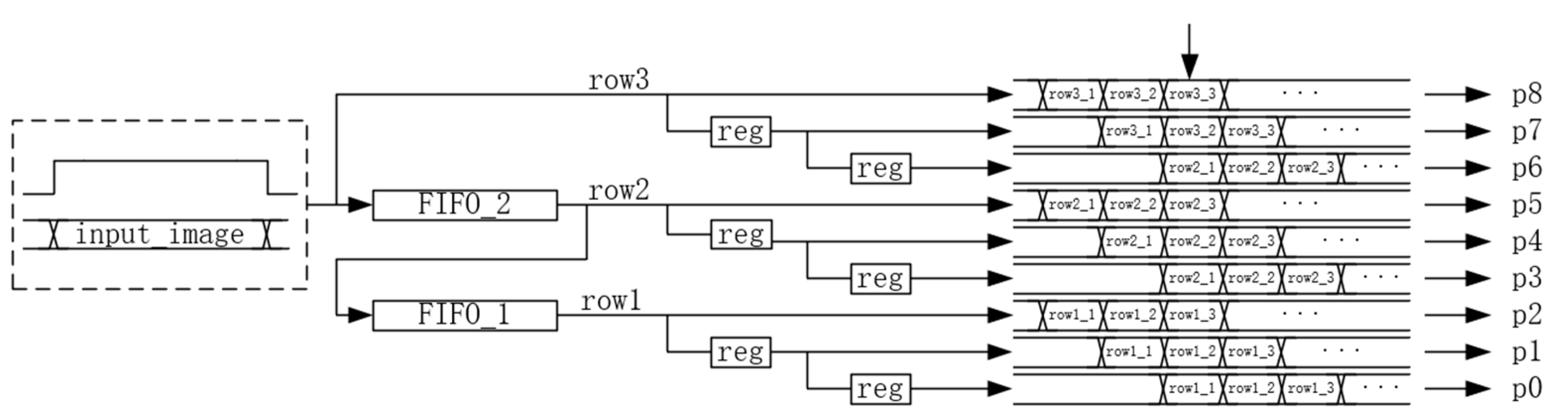
2.2.3. Non maximum Suppression

Non maximum suppression (NMS) is an edge-thinning technique for preserving local maxima along the image gradient direction. Figure 9 shows the NMS architecture. The selector is used to find the pixels in the direction equivalent to the current pixel (center pixel of 3 × 3 window) direction depicted as a and b in Figure 9. For directions 1 or 8, the values of a and b are g3 and g5; for directions 2 or 3, the values of a and b are g0 and g8; for directions 4 or 5, the values of a and b are g5, and g6; for directions 6 or 7, the values of a and b are g1 and g7; The comparator (CMP) is used to compare the current pixel (g4) with a and b to determine the presence of maxima. If the maxima are present in the current pixel, then it is preserved. Otherwise, it is suppressed as 0. Considering that the maximum value of g4 requires 10 bits, to save hardware resources for later statistics, we limit the value range to 8 bits. The value generated after the NMS is sent to both the data cache module and the adaptive threshold computation module, as shown in Figure 2. Data can be cached inside the FPGA or outside the FPGA. Here, data are cached in external SDRAM.

2.2.4. Adaptive Threshold Computation

Adaptive threshold calculation is the most important part of the proposed canny edge detector system. After NMS, we used Otsu’s algorithm to adaptively calculate the threshold we needed. Since the NMS data needs to be compared with the calculated threshold, the threshold value can only be obtained after the statistics of the entire image. Therefore, the NMS data needs to be cached in advance, which is completed by the SDRAM controller. For the threshold calculation, the relevant parameters of Otsu’s algorithm were obtained through histogram statistics, and then the threshold was calculated. After the threshold calculation was completed, SDRAM signal reading was enabled at the same time. Then the NMS data was compared with the threshold value for binarization, and finally, the hysteresis was carried out. Figure 10 shows the flow diagram of the system after NMS, including data caching, histogram statistics, threshold calculation, binarization, and hysteresis.

(1)

Otsu’s Algorithm

Otsu’s algorithm [18] is a popular thresholding algorithm used to find an optimal threshold that separates an image into two classes: the background and the object. These classes are represented by C0 and C1, respectively. This method performs a variance analysis processing to find the optimal threshold k by a maximization, as shown in Equation (10).

$$\begin{array}{c}k=\begin{array}{c}arg \max \left({\sigma }_k^2\right)\\ 0\le k\le L-1\end{array}\end{array}$$

(10)

where ${\sigma }_k^2$ is the k-th between-class variance of the image, defined as:

$$\begin{array}{c}{\sigma }_k^2=\frac{{\left(u_{L-1}\times w_k-u_k\right)}^2}{w_k\left(1-w_k\right)}\end{array}$$

(11)

where $w_k$ and $u_k$ are the probability of class occurrence given a k threshold and the mean intensity value of the pixels up to the k threshold of the image, respectively, and $u_{L-1}$ is the average intensity of the entire image, called the global mean, with a value equal to $u_k$ when k = L − 1. Normally, L is equal to 256.

The variables $w_k$ and $u_k$ can be expressed as

$$\begin{array}{c}{w}_k={\displaystyle {\displaystyle \sum }_{i=0}^k}{p}_i\end{array}$$

(12)

and

$$\begin{array}{c}{u}_k={\displaystyle {\displaystyle \sum }_{i=0}^k}i\times p_i\end{array}$$

(13)

(2)

Logarithm Approximation

The division operation is costly to the hardware in terms of processing speed and is the architecture’s bottleneck due to the highest critical time. To avoid the division operation in Equation (11), the logarithm function is presented in [26,27], and Equation (11) can be accordingly rewritten as:

$$\begin{array}{c}2lo{g}_2\left({\sigma }_k\right)=2lo{g}_2\left(u_{L-1}\times w_k-u_k\right)-lo{g}_2\left(w_k\right)-lo{g}_2\left(1-w_k\right)\end{array}$$

(14)

(3)

Architecture of adaptive threshold computation

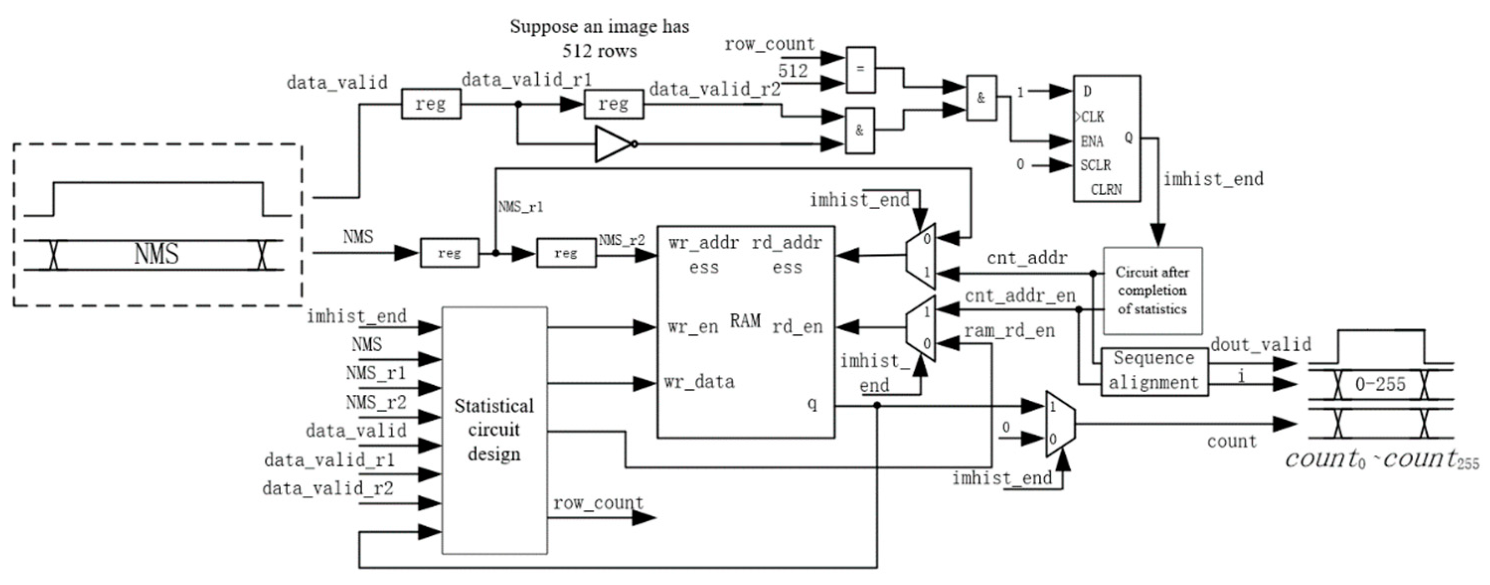
(a)

Architecture of histogram

The histogram is the key part of Otsu’s algorithm. Histogram statistics are performed on a series of values generated by the NMS. Figure 11 shows the architecture of the histogram. Here, we used a RAM, and the address bit width is 8 bits. The data bit width can be flexibly selected according to the number of pixels in the image. Thirty-two bits are used here. The architecture is divided into two parts. The first part is before the completion of statistics, and the other part is after the completion of statistics. The steps for computing the histogram statistics are as follows:

(1)

Read out the current statistics, add 1 and write them back to RAM.

(2)

Repeat the above steps until the current image has been counted. If imhist_end is 1, as shown in Figure 11, the statistics are complete.

(3)

Next, start reading out the data in order.

Step (1) is realized by the statistical circuit module, and step (3) is realized by the circuit after completion of the statistics module, as shown in Figure 11.

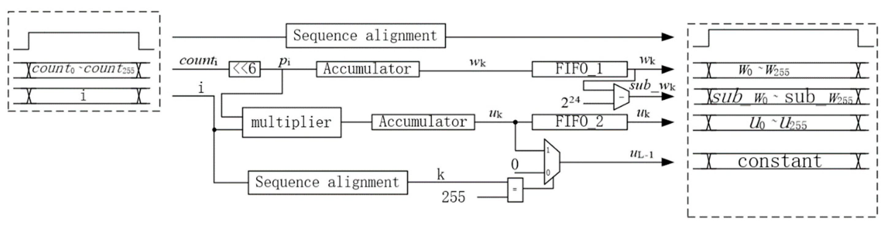
(b)

Architecture of Otsu’s algorithm calculation

After the statistics were completed, parameters $u_{L-1}$, $u_k$ and $w_k$ in Otsu’s algorithm were calculated. Before the calculation, a normalized cumulative histogram is needed. Here, we use the fixed-point number system [19] to represent non-integers. Figure 12 shows 32-bit (16.16) unsigned fixed-point numbers. In the proposed architecture, a 32-bit (8.24) unsigned fixed-point number system is used.

Since we use 24 bits as the fractional part, the value of $p_i$ in Equation (12) can be calculated as follows:

$$\begin{array}{c}{p}_i=\frac{coun{t}_i}{total\_piexls\_num}\times 2^{24} 0\le i\le 255\end{array}$$

(15)

In this paper, all images are 512 × 512 in size, so the value of $p_i$ can be obtained by shifting $coun{t}_i$ six places to the left. The value of $coun{t}_i$ is calculated in the histogram, as shown Figure 11. Figure 13 shows the architecture of Otsu’s algorithm calculation.

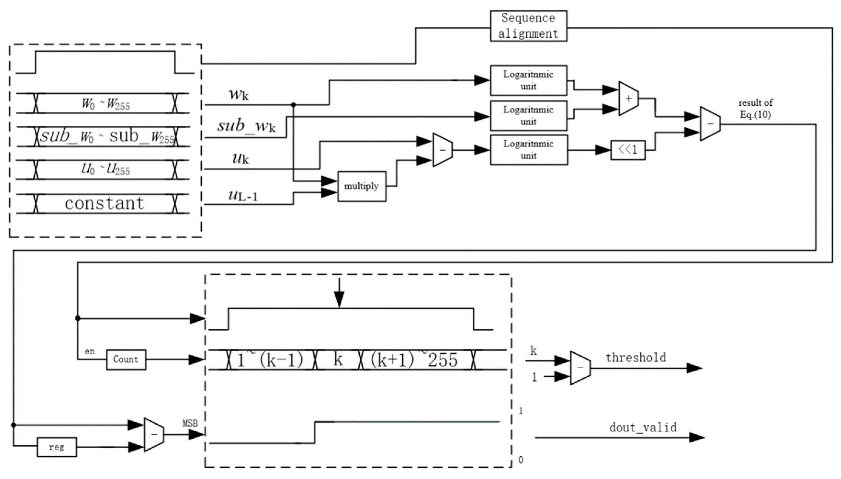
(c)

32-bit Logarithmic Arithmetic Unit

The logarithmic number system (LNS) has been studied to simplify arithmetic computations to achieve a lower computation complexity [26,27,28]. Here, a 32-bit logarithmic arithmetic unit suggested in [28] is adopted to compute Equation (14). Figure 14 shows the architecture of the logarithmic converter. It is composed of a 32-bit count leading zero (CLZ), a barrel shifter (BSH), a characteristic generator (CGen), and a fractional part generation block (FPGen). The variable input number range Qm.n. is modified to the fixed number range of Q6.26. at the end of the logarithmic converter. The CLZ block calculates the number of leading zero bits of the input. The five bits of the CLZ block output determine the characteristic value and the amount of shift value of the BSH. BSH converts the input number range of Qm.n. to Q6.26. After the shifting operation, the fractional part is generated by the FPGen block, and the characteristic part is generated by the CGen block. The above two values are combined to give the logarithmic conversion result.

(d)

Threshold calculation

Figure 15 shows the architecture of the threshold calculation. When the result of $2lo{g}_2{\sigma }_k$ is obtained, the value of k corresponding to the first negative value (when the MSB of the result is 1) is found by subtracting the values before and after. Finally, the obtained k value is reduced by one to obtain the optimal threshold. The output signal dout_valid in Figure 15 is equal to the threshold calculated in Figure 2, and the purpose is to enable the output to obtain temporarily cached NMS values.

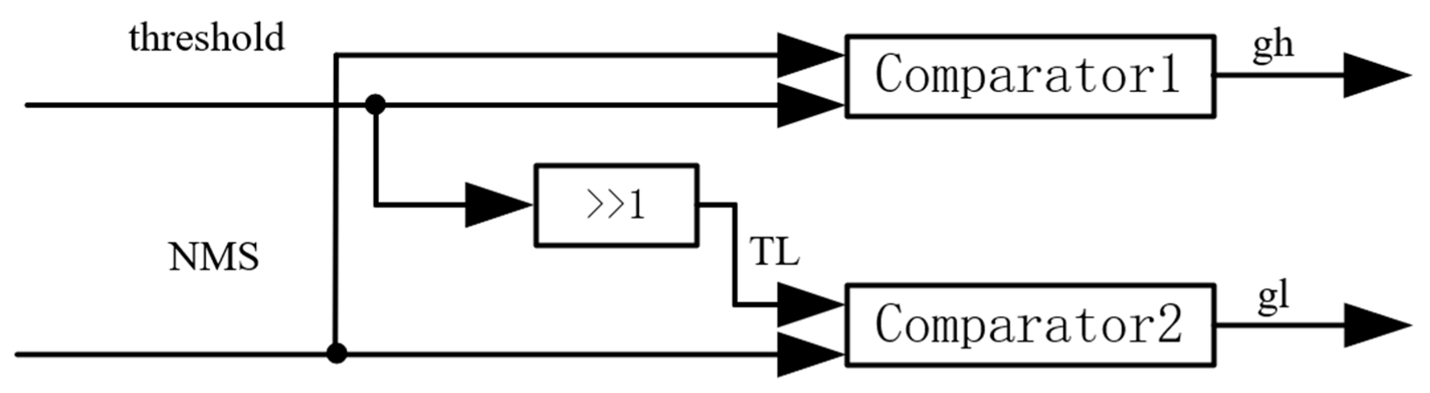
2.2.5. Binarization

After the threshold calculation is completed, the value obtained is set as the high threshold value, and the low threshold value is half of it. Then, the comparison is conducted to find the strong edge and the weak edge. Figure 16 shows the architecture of binarization, where gh represents the strong edge and gl represents the weak edge.

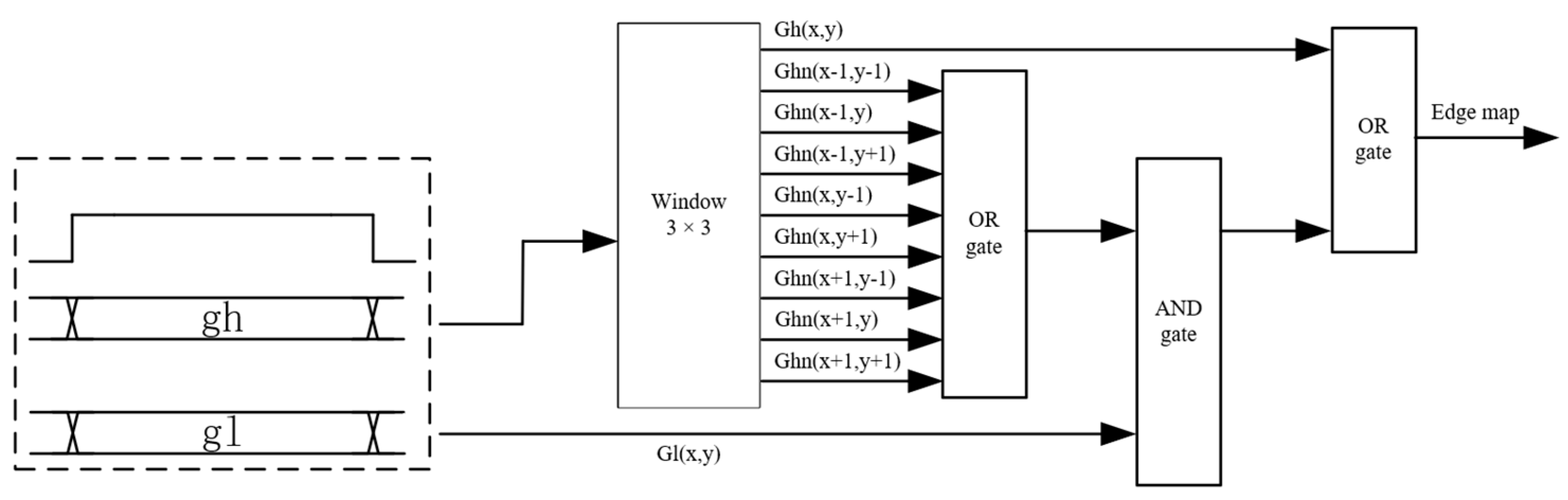
2.2.6. Hysteresis

The non maximum suppression technique finds strong edges. The edges affected by noise and illumination changes are preserved by this technique. After obtaining the values of gh and gl, if gh is 1, the gradient magnitude value is a strong edge pixel and is preserved. If gl is 0, it is not an edge pixel. If gl is 1, which means the gradient magnitude value is a weak edge pixel, then the current pixel is considered a strong edge pixel if and only if any of the neighbors of the current pixel depicted as Ghn with various coordinate values in Figure 17 is a strong edge pixel. Otherwise, it is a weak edge pixel and is suppressed. Figure 17 shows the architecture of hysteresis thresholding.

3. Experimental Results and Analysis

The proposed architecture of the Canny edge detection algorithm is tested on a grayscale image size of 512 × 512 from Standard Test Image Database [29], which is implemented using Intel Quartus Prime 18.0 and is verified on Altera’s Cyclone IV E: EP4CE10F17C8 FPGA board.

The proposed technique uses (1) an approximation technique for the computation of gradient magnitude and orientation, (2) Otsu’s algorithm adaptively calculates threshold (3) a logarithmic operation unit is introduced to reduce the complexity of Otsu’s algorithm.

3.1. Performance Analysis

Figure 18 shows the Sobel edge map using different magnitude calculation equations (Equations (3) and (5)). It can be seen from Figure 18 that different calculation equations will make the intensity of edge pixels different. The intensity of edge pixels calculated by the Equation (5) is generally greater than that of Equation (3). However, this does not affect subsequent NMS operations.

A comparison of the quality of the NMS map due to the use of quantized tanh is shown in Figure 19. As shown in Figure 19, the quality of the NMS image is not affected by the use of quantified tanh, which means that the gradient direction can be found correctly using this technique during the NMS process.

Since we introduced logarithmic approximation into the architecture, a comparison was made between using and not using logarithmic approximation. As shown in Figure 20, the edge map using logarithmic approximation is basically the same as that without logarithmic approximation, which verifies the feasibility of using this technique.

The performance of traditional Canny edge detection with a fixed threshold is compared with the performance of the proposed Canny edge detection algorithm. Illumination variation is a challenging task to detect the edges since the edges present in an image are sensitive to variation in light intensity that might occur because of various local and global lighting conditions. Therefore, the performance is evaluated at various illumination. Figure 21 shows the comparison results of traditional and proposed Canny edge detection algorithms. Figure 21a shows the grayscale of an image under different illumination. Figure 21b shows the edge map detected by the Canny edge detection algorithm with a fixed threshold value, which is implemented in MATLAB. The Gaussian kernel used is 9 in size and 1.5 in standard deviation, and the fixed threshold value is 70. Figure 21c shows the edge map detected by the proposed Canny edge detection algorithm.

It is observed from Figure 21 that the proposed algorithm shows better performance under various illumination conditions than traditional Canny edge detection with a fixed threshold. This is due to the fact that the proposed edge detection algorithm in this research utilizes adaptive threshold technology to reduce the impact of light variations on the detection effect.

3.2. Resource Utilization

In this section, the resource utilization of the proposed algorithm is analyzed since the system must utilize less hardware for real-time requirements.

Table 2. Comparison of resource utilization and computation time.

Edge Detection Methods	Image Size	FPGA Device	Used Slices	Memory Used (KB)	Max Freq. (MHz)	Time (ms)	Norm. Time (ms)
[6]	512 × 512	Xilinx Virtex-5	4553	192	292	0.57	3.338
[7]	360 × 280	Altera Cyclone	-	-	27	2.5	1.44
[8]	512 × 512	Xilinx Virtex-5	23904	16184	250	0.15	0.774
[9]	512 × 512	Xilinx Virtex-5	17928	278	272	0.13	0.54
proposed	512 × 512	Altera Cyclone IV	3303	261	56.7	1.231	1.231

illustrates the resource utilization comparison of the proposed Canny edge detection algorithm with other Canny edge detection algorithms. Observations show that compared with the implementation [6], the proposed architecture uses less hardware due to the approximation of complex operations, but more storage resources are used because the implementation [6] uses a fixed threshold which degrades the performance of edge detection while our architecture uses an adaptive threshold that requires caching of the entire image. For the implementation [7,8], they divide an image into several blocks and then use the Canny edge detection algorithm for each block in parallel, which greatly reduces latency and has an absolute advantage in terms of processing speed. However, at the same time, the consumption of hardware resources also increases sharply.

3.3. Execution Time

Compared with other existing techniques. The simulation result shows that it takes about 1.231 ms to detect edges of the image at an operating frequency of 50 MHz, which is sufficient for real-time applications.

As far as we know, the existing FPGA-based approaches implemented the Canny algorithm, and only the computation time for detecting edges is presented in papers [6,7,8,9]. The computation time and resource utilization results of these Canny FPGA implementations and our Canny FPGA implementation are shown in Table 2. Since these approaches are implemented for different image sizes and operated at different clock frequencies, their results have to be normalized for a fair comparison. The rightmost column of Table 2 gives the normalized computing time, where the normalization is done with respect to an image of size 512 × 512 and an FPGA clock frequency of 50 MHz. Although the execution time of this algorithm is twice that of reference [6], we use fewer logical resources. In addition, since reference [6] uses a fixed threshold, this paper adopts an adaptive threshold technology, so the detection effect in this paper is better than that in reference [6]. In comparison to the algorithm in this paper, the Canny edge detection algorithm based on block structure in [8,9] substantially decreases detection time but greatly increases resources. As a result, the technique suggested in this research is better suited for platforms with limited hardware resources.

Table 3. Run time comparison of GPGPU and proposed FPGA implementation.

	GTX 80 [15]	GT 80 [17]	GT 200 [17]	Fermi [17]	Proposed
Image size	512 × 512	321 × 481	321 × 481	321 × 481	512 × 512
Freq (MHz)	768	1500	1300	1150	50
Time (ms)	3.4	5.47	2.95	2.3	1.231
Norm. time (ms)	52.224	278.62	130.22	89.82	1.231

illustrates a run time comparison of GPGPU implementation and proposed FPGA implementation. Even though the proposed FPGA implementation uses adaptive threshold value and operates at a lower frequency, it is faster than GPGPU implementation. The GPU configuration details are given below.

▪

GTX 80 [15]: NVidia GeForce 8800 GTX with 128 575-MHz cores and 768 MB RAM.

▪

GT 80 [17]: NVidia GeForce 8800 GT with 112 1.5-GHz cores and 512 MB RAM.

▪

GT 200 [17]: NVidia Tesla C1060 with 240 1.3-GHz cores and 4 GB RAM.

▪

Fermi [12]: NVidia Tesla C2050 with 448 1.15-GHz cores and 3 GB RAM.

4. Conclusions

In this paper, an improved Canny edge detection algorithm is proposed and implemented on an FPGA. In this new Canny edge detector, an approximate method is used to reduce the complexity of computing the gradient magnitude and orientation, facilitate hardware implementation, and reduce resource usage. In addition, Otsu’s algorithm is used to adaptively determine the image threshold. Compared with the fixed threshold scheme, this results in better edge detection performance under the condition of a variable detection environment. Due to the high complexity of Otsu’s algorithm, it is difficult to implement it directly on FPGA. Therefore, the logarithmic operation unit is introduced to reduce the complexity of Otsu’s algorithm, which further simplifies the hardware architecture and reduces resource usage. The result shows that the proposed algorithm’s implementation requires only 1.231 ms to detect the edges of the 512 × 512 image when clocked at 50 MHz. In addition, the proposed hardware architecture uses the fewest logical resources and is more suitable for hardware platforms with limited resources. In the future, this system can be a candidate for real-time edge detection applications.

References

- Roberts, L.G. Machine perception of 3D solids. In Optical and Electro-Optical Information Processing; MIT Press: Cambridge, MA, USA, 1965. [Google Scholar]
- Gonzalez, R.C.; Woods, R.E. Digital Image Processing; Pearson Education Inc.: London, UK; Prentice Hall: Hoboken, NJ, USA, 2008. [Google Scholar]
- Kanopoulos, N.; Vasanthavada, N.; Baker, R.L. Design of an image edge detection filter using the sobel operator. IEEE J. Solid-State Circuits 1988, 23, 358–367. [Google Scholar] [CrossRef]
- Davies, E.R. Constraints on the design of template masks for edge detection. Pattern Recognit. Lett. 1986, 4, 111–120. [Google Scholar] [CrossRef]
- Canny, J. A computation approach to edge detection. IEEE Trans. Pattern Anal. Mach. Intell. 1986, 8, 679–698. [Google Scholar] [CrossRef] [PubMed]
- Gentsos, C.; Sotiropoulou, C.L.; Nikolaidis, S. Real-Time Canny Edge Detection Parallel Implementation for FPGAs. In Proceedings of the 17th IEEE International Conference on Electronics, Circuits and Systems (ICECS), Athens, Greece, 12–15 December 2010; pp. 499–502. [Google Scholar]
- He, W.; Yuan, K. An Improved Canny Edge Detector and its Realization on FPGA. In Proceedings of the 7th World Congress on Intelligent Control and Automation (WCICA), Chongqing, China, 25–27 June 2008; pp. 6561–6564. [Google Scholar]
- Xu, Q.; Varadarajan, S.; Chakrabarti, C. A Distributed Canny Edge Detector: Algorithm and FPGA Implementation. IEEE Trans. Image Process. 2014, 23, 2944–2960. [Google Scholar] [CrossRef] [PubMed]
- Sangeetha, D.; Deepa, P. FPGA implementation of cost-effective robust Canny edge detection algorithm. J. Real-Time Image Proc. 2019, 16, 957–970. [Google Scholar] [CrossRef]
- Deriche, R. Using Canny Criteria to derive a recursively implemented optimal Edge detector. Int. J. Comput. Vis. 1987, 1, 167–187. [Google Scholar] [CrossRef]
- Torres, L.; Robert, M.; Bourennane, E.; Paindavoine, M. Implementation of a Recursive Real Time Edge Detector Using Retiming Technique. In Proceedings of the Asia and South Pacific IFIP International Conference on Very Large Scale Integration, Chiba, Japan, 29 August–1 September 1995; pp. 811–816. [Google Scholar]
- Lorea, F.G.; Kessal, L.; Demigny, D. Efficient ASIC and FPGA implementation of IIR filters for Real Time Edge Detection. In Proceedings of the IEEE International Conference on Image Processing (ICIP-97), Santa Barbara, CA, USA, 26–29 October 1997; Volume 2, pp. 406–409. [Google Scholar]
- Park, I.K.; Singhal, N.; Lee, M.H.; Cho, S.; Kim, C.W. Design and performance evaluation of image processing algorithms on GPUs. IEEE Trans. Parallel Distrib. Syst. 2011, 22, 91–104. [Google Scholar] [CrossRef] [Green Version]
- Owens, J.D.; Luebke, D.; Govindaraju, N.; Harris, M.; Kruger, J.; Lefohn, A.E.; Purcell, T.J. A survey of general-purpose computation on graphics hardware. Comput. Graph. Forum 2007, 26, 80–113. [Google Scholar] [CrossRef] [Green Version]
- Luo, Y.; Duraiswami, R. Canny edge detection on NVIDIA CUDA. In Proceedings of the 2008 IEEE Computer Society Conference on Computer Vision and Pattern Recognition Workshop (CVPRW), Anchorage, AK, USA, 23–28 June 2008; pp. 1–8. [Google Scholar]
- Palomar, R.; Palomares, J.M.; Castillo, J.M.; Olivares, J.; GomezLuna, J. Parallelizing and optimizing lip-Canny using NVIDIA CUDA. In IEA/AIE 2010: Trends in Applied Intelligent Systems, Proceedings of the 23rd International Conference on Industrial Engineering and Other Applications of Applied Intelligent Systems, Cordoba, Spain, 1–4 June 2010; Springer: Berlin/Heidelberg, Germany, 2011; pp. 389–398. [Google Scholar]
- Lourenco, L.H.A. Efficient implementation of Canny edge detection filter for ITK using CUDA. In Proceedings of the 13th Symposium on Computer Systems, Petropolis, Brazil, 17–19 October 2012; pp. 33–40. [Google Scholar]
- Otsu, N. A threshold selection method from gray-level histograms. IEEE Trans. Syst. Man. Cybern. 1979, 9, 62–66. [Google Scholar] [CrossRef] [Green Version]
- Pandey, J.G.; Karmakar, A.; Shekhar, C. A Novel Architecture for FPGA Implementation of Otsu’s Global Automatic Image Thresholding Algorithm. In Proceedings of the 27th International Conference on VLSI Design and 13th International Conference on Embedded Systems, Mumbai, India, 5–9 January 2014; pp. 300–305. [Google Scholar]
- Albert, F.; Monsalve, T.; Median, J.V. Hardware implementation of ISODATA and Otsu thresholding algorithms. In Proceedings of the XXI Symposium on Signal Processing, Images and Artificial Vision (STSIVA), Bucaramanga, Colombia, 31 August–2 September 2016; pp. 1–5. [Google Scholar]
- Zhang, H.; Wang, S.Z.; Zheng, Y.; Wang, W.; Li, W.Z.; Wang, P.; Ren, G.S.; Ma, J.L. FPGA implementation of image edge detection based on four algorithms of GAUSS-filter, Sobel, NMS and OTSU. Chin. J. Liq. Cryst. Disp. 2020, 35, 250–261. [Google Scholar] [CrossRef]
- Sun, J.C.; Wang, Z.Y.; Li, Z.G. Implementation of Sobel Edge Detection algorithm and VGA display based on FPGA. In Proceedings of the IEEE 4th Advanced Information Technology, Electronic and Automation Control Conference (IAEAC), Chengdu, China, 20–22 December 2019; pp. 2305–2310. [Google Scholar]
- Tippett, J.T.; Borkowitz, D.A.; Clapp, L.C.; Koester, C.J.; Vanderburgh, J.A. Optical and Electro-Optical Information Processing; MIT Press: Cambridge, MA, USA, 1965. [Google Scholar]
- Bruguera, J.D.; Gull, N.; Lang, T. CORDIC based parallel/pipelined architecture for the Hough transform. J. VLSI Signal Process. Syst. Signal Image Video Technol. 1996, 12, 207–221. [Google Scholar] [CrossRef] [Green Version]
- Ngo, H.T.; Asari, V.K. A Pipelined Architecture for Real-Time Correction of Barrel Distortion in Wide-Angle Camera Images. IEEE Trans. Circuits Syst. Video Technol. 2005, 15, 436–444. [Google Scholar] [CrossRef]
- Abed, K.H.; Siferd, R.E. CMOS VLSI Implementation of a Low-Power Logarithmic Converter. IEEE Trans. Comput. 2003, 52, 1421–1433. [Google Scholar] [CrossRef]
- Kim, H.; Nam, B.G.; Sohn, J.H.; Woo, J.H.; Yoo, H.J. A 231-MHz, 2.18-mW 32-bit Logarithmic Arithmetic Unit for Fixed-Point 3-D Graphics System. IEEE J. Solid-State Circuits 2006, 41, 2373–2381. [Google Scholar] [CrossRef]
- Abed, K.H.; Siferd, R.E. CMOS VLSI Implementation of 16-bit Logarithm and Anti-logarithm Converters. In Proceedings of the IEEE 43rd Midwest Symposium on Circuits and Systems, Lansing, MI, USA, 8–11 August 2000; pp. 776–779. [Google Scholar]
- Standard Test Image Database. Available online: http://www.imageprocessingplace.com/ (accessed on 24 May 2015).