Article

Research and Implementation of High Computational Power for Training and Inference of Convolutional Neural Networks

College of Information Science and Technology, Beijing University of Chemical Technology, Beijing 100029, China
*
Author to whom correspondence should be addressed.
Appl. Sci. 2023, 13(2), 1003; https://doi.org/10.3390/app13021003
Submission received: 17 November 2022 / Revised: 1 January 2023 / Accepted: 9 January 2023 / Published: 11 January 2023
(This article belongs to the Special Issue Intelligent Computing and Remote Sensing)

Abstract

:
Algorithms and computing power have consistently been the two driving forces behind the development of artificial intelligence. The computational power of a platform has a significant impact on the implementation cost, performance, power consumption, and flexibility of an algorithm. Currently, AI algorithmic models are mainly trained using high-performance GPU platforms, and their inferencing can be implemented using GPU, CPU, and FPGA. On the one hand, due to its high-power consumption and extreme cost, GPU is not suitable for power and cost-sensitive application scenarios. On the other hand, because the training and inference of the neural network use different computing power platforms, the data of the neural network model needs to be transmitted on platforms with varying computing power, which affects the data processing capability of the network and affects the real-time performance and flexibility of the neural network. This paper focuses on the high computing power implementation method of the integration of convolutional neural network (CNN) training and inference in artificial intelligence and proposes to implement the process of CNN training and inference by using high-performance heterogeneous architecture (HA) devices with field programmable gate array (FPGA) as the core. Numerous repeated multiplication and accumulation operations in the process of CNN training and inference have been implemented by programmable logic (PL), which significantly improves the speed of CNN training and inference and reduces the overall power consumption, thus providing a modern implementation method for neural networks in an application field that is sensitive to power, cost, and footprint. First, based on the data stream containing the training and inference process of the CNN, this study investigates methods to merge the training and inference data streams. Secondly, high-level language was used to describe the merged data stream structure, and a high-level description was converted to a hardware register transfer level (RTL) description by the high-level synthesis tool (HLS), and the intellectual property (IP) core was generated. The PS was used for overall control, data preprocessing, and result analysis, and it was then connected to the IP core via an on-chip AXI bus interface in the HA device. Finally, the integrated implementation method was tested and validated with the Xilinx HA device, and the MNIST handwritten digit validation set was used in the tests. According to the test results, compared with using a GPU, the model trained in the HA device PL achieves the same convergence rate with only 78.04 percent training time. With a processing time of only 3.31 ms and 0.65 ms for a single frame image, an average recognition accuracy of 95.697%, and an overall power consumption of only 3.22 W @ 100 MHz, the two convolutional neural networks mentioned in this paper are suitable for deployment in lightweight domains with limited power consumption.

1. Introduction

In recent years, convolutional neural networks have been widely used in speech recognition, image classification, image processing, accelerators, demodulators, etc., and have shown great advantages, especially in image classification [1,2]. At present, there are various convolutional neural network algorithms in deployment, but due to the sheer amount of computation required, the implementation of traditional convolutional neural networks has mostly been based on the more ideal PC framework and has been trained by GPUs. However, GPUs’ low flexibility, extreme cost, and power consumption have limited their application in certain scenarios [3,4], such as cases where it would be difficult to integrate GPUs in tiny mobile devices and aerospace applications [5]. Therefore, the modest size of FPGAs has attracted the attention of researchers. Traditional hardware system implementations involve numerous serial computations, while FPGAs can realize all parallel computing when there are sufficient logic units, which considerably improves the computing speed when using FPGAs to process relevant data [6,7]. Compared with the data parallel operation of GPUs, FPGAs add pipeline parallelism on the basis of data parallelism. Therefore, more and more researchers have begun to use FPGA to implement CNN algorithms.
With the increasing demand for computing power, FPGA has increasingly been used in the inferencing implementation of artificial intelligence models, where it accelerates the forward inference of neural networks and significantly reduces the power consumption of devices. However, hardware acceleration schemes for pure FPGA implementations of CNN inevitably lead to the separation of training and the inference. To some extent, this reduces the flexibility and adaptability of the neural network, and the dynamic control of the neural network during training cannot be achieved. In recent years, the emergence of HA devices with FPGA at their core has provided a new way to realize the integration of high computing power for AI training and inference. The processing system (PS) and PL are integrated into the HA device. On the one hand, the hybrid structure has great flexibility and enables dynamic control of the neural network training and inference process. On the other hand, this construction has strong parallel inference capabilities. As a result, the performance of neural network training and inference is significantly improved, which provides a different solution for the training and inference of AI models.
Researchers have begun to implement FPGA-based HA SoC to realize the hardware acceleration and miniaturization deployment of a neural network and to use the multicore processor of HA SoC for training and the programmable logic part for reasoning, to reduce power consumption, save costs, and improve performance [8,9,10]. However, compared to forward inference, the multiplication and addition operations of neural networks are computationally intensive. Therefore, the data preprocessing and data stream management operations in the PS of HA SoC can give full play to its flexibility, and the training and inference of the neural network in the PL of HA SoC can give full play to its parallel operation characteristics and significantly improve the overall performance of the system. Figure 1 shows the proposed ensemble neural network training and inference method.
To sum up, the main contributions of this paper are listed as follows:
  • Based on the features of HA SoC, a new neural network implementation method is proposed to balance a load of software and hardware by introducing the co-design of software and hardware. Considering the flexibility of software and the parallel processing ability of hardware, the integrated neural network training and inference process is realized.
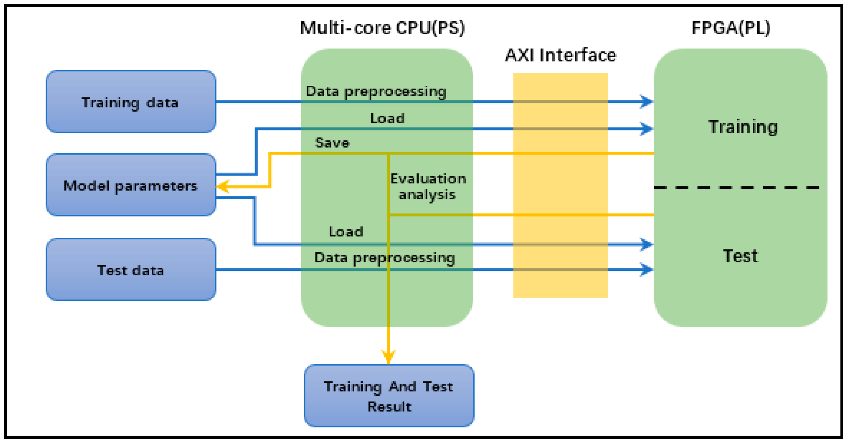
  • In this implementation, PL is used to realize the training and inference process of the neural network, and PS is used to realize the scheduling of the whole process of training and inference including data preprocessing.
  • Pipelining and parallelism are weighed within PL in terms of limited logical resources, according to the data flow structure of training and inference. On the premise of ensuring the forward inference and training accuracy of the neural network, the training process of the neural network is accelerated as much as possible.
The rest of the study in this paper is as follows: Section 2 presents some related seminal works. Section 3 introduces the LeNet-3.3 and Le-Net-2.22 convolution neural network models and data flow structures for MNIST data set recognition, proposes the overall design scheme of the integration of training and inference of the neural network on HA SoC, and gives the architectural features of the design and the distribution strategy of software and hardware load. In Section 4, the high-level description methods of the above two neural networks are detailed and the RTL structure transformed by the HLS tool is optimized. Finally, IP cores containing training and inference are generated. In the Section 5, a hardware test environment for testing IP core function and performance is built based on HA architecture SoC devices, and the function test and performance evaluation of the IP core is carried out from the aspects of resource consumption, device power consumption, model convergence speed, training duration, inference accuracy, and inference duration. Section 6 analyzes the performance of the IP core based on the test results and compares it with current mainstream GPU implementation approaches. Finally, the contributions of the paper are summarized, and future research directions are planned.

2. Related Work

The development of convolutional neural networks dates back to 1962 when Hubel and Wiesel proposed the concept of receptive fields through their study of the visual system in the cat brain. In 1980, Japanese scientist Unitika Fukushima proposed a neural network architecture consisting of a convolutional layer and a pooling layer. He also proposed the concept and the network of attention in the 1980s. In 1998, Yann LeCun proposed LeNet-5 on this basis and applied the BP algorithm to the training of this neural network structure, thus forming the prototype of a contemporary convolutional neural network [1].
MNIST is a large data set containing digits, and upper- and lower-case handwritten letters. The MNIST data set is a large handwritten character data set from MNIST, including handwritten digit pictures from 0 to 9, with 60,000 training images and 10,000 test images. The image size is 28 × 28 pixels, and it is a single-channel grayscale image. This data set is often used to train various image processing systems and is widely used in the field of deep learning [11].
With the development of deep learning, a convolution neural network (CNN) has gradually become one of the mature algorithms in the field of artificial intelligence. However, the computational complexity of CNN is also higher than traditional algorithms, and the network structure is increasingly complex. A growing number of researchers are seeking hardware acceleration methods for CNN. Guo K and Sui L proposed Angel-Eye, which is a programmable and flexible CNN accelerator architecture [12]. It is a design procedure that maps the CNN to an embedded FPGA and implements the forward inference process of the CNN through the FPGA to achieve a local speedup of the CNN. However, the flexibility of a pure FPGA accelerator is significantly lower than that of an FPGA-based HA SoC. Multicore high-performance ARM processors integrated into HA SoC can complete the training process of neural networks, and PL-accelerated forward inference in HA SoC can achieve the full training and inference process of neural networks.
Neural network deployment based on HA SoC has gradually become a hot topic. Gschwend D implemented an efficient CNN topology ZynqNet on a Zynq on-chip system [13]. ZynqNet is a miniature embedded neural network specially designed for image classification. It trained and optimized exclusive CNN in PS and realized forward inference acceleration of CNN in PL. The accuracy of hardware-accelerated CNN is higher than 84.5% and the computational complexity is only 530 million times multiplication. Yangyang Zheng implemented forward inference acceleration of the LeNet-5 network based on Xilinx MPSoC [14]. Finally, the recognition accuracy of the MNIST data set and the CIFAR-10 data set reached 99.5% and 75.4%, respectively, and the average processing time of a single frame was only 2.2ms. Numerous studies have shown that HA SoC has better flexibility, which is conducive to the training and inference of the implementation and deployment of neural networks and is superior to alternative implementation schemes in terms of performance and power consumption [15,16,17].
To sum up, hardware acceleration based on HA SoC makes the inference of neural networks more flexible, but few researchers use PL to accelerate the training process of the neural network [18,19,20,21]. Therefore, the integration of model training and forward inference cannot be realized, which will significantly improve the overall system performance and reduce the total cost and power consumption of the system [22]. In HA SoC, the flexibility of software and the parallel processing of hardware are profoundly integrated. The software running in the PS is responsible for data preprocessing and controlling the data flow. PL performs complex data operations during training and inference. This provides another realization method to further optimize the computing power of AI in terms of performance, cost, power consumption, flexibility, and adaptability [18,23].

3. Method

3.1. Integrated Architecture of Neural Network Training and Inference

As shown in Figure 2, in the integrated implementation architecture, the PS and PL resources in the HA SoC are allocated according to the training and inference data streams. This architecture is divided into four parts: (1) under the scheduling of the operating system, PS is responsible for controlling the process of training and inference, completing the pre-processing of training and inference data, randomly initializing the network weight, updating the weight file, and evaluating the training and inference results; (2) through internal reuse, the hardware training and inference process is realized in PL. (3) Through the advanced extended interface (AXI) interface, the training data and initial network weights are loaded into the PL. In the PL, the model is trained to produce the final network weights. These weights are retained in the PL to facilitate subsequent training; at the same time, they are also fed back to PS to evaluate the training effect. (4) Load the data needed for inference into the PL through the AXI interface, perform model inference in the PL, and return the final result obtained by inference to PS.

3.2. Training and Inference of Neural Networks

The training and inference data used in this design is a 30 × 30 pixel single-channel grayscale map. Due to the small amount of data, this design proposes two improved network models based on the classical convolutional neural network LeNet-5 (hereinafter referred to as LeNet-3.3 and LeNet-2.22) to analyze the performance of different network structures in the integrated implementation method. The LeNet-3.3 network removes the pooling layer, increases network complexity and image feature information, and studies the advantages of complex networks in this implementation method. The LeNet-2.22 network adopts the method of reducing the number of network weights and studies the advantages of a simple network in this implementation method.
The network model of LeNet-3.3 is shown in Figure 3. The convolutional neural network has six network layers; the first three are regular layers and the input is a 30 × 30 pixel feature map based on a single channel of the modified MNIST data set. After each conditioning layer, the max pooling layer is removed to retain all of the feature map information. The next three layers are fully connected, and the last layer completes the image classification output. The convolutional neural network uses the modified ReLU function as the activation function. The output of the output layer is normalized via the Soft Max function.
The network model of LeNet-2.22 is shown in Figure 4. The convolutional neural network has six network layers, the first four of which alternate between convolutional and pooling layers. The last two layers are fully connected, and the last layer completes the image classification output. The neural network also uses the same activation functions, ReLU and Soft Max, as the LeNet-3.3 network.
Figure 5 shows the data flow structure of image data forward propagation and gradient loss backpropagation in the LeNet-3.3 network. In the figure, the forward propagation of image data is used to train the model, and the backpropagation of gradient loss is used for model inference. In essence, the training of neural networks includes both the forward propagation of data and the backpropagation of gradient loss. Therefore, the inference of convolution neural networks is a part of model training, which is a prerequisite for the integration of training and inference in PL. In the integrated structure of training and inference, the trained network weights are stored in the corresponding RAM and can be directly used in inference without PS intervention. In essence, the integrated structure of training and inference significantly reduces the cost and power consumption of the computing power platform, while improving the flexibility, reliability, and real-time performance of the whole system, providing a new solution for the training and inference of artificial intelligence.
To balance the software and hardware design resources in the HA SoC, the integrated structure of the convolutional neural network is split. The training and inference of convolutional neural networks involve the following external operations, including the management of image data and weight files, image data preprocessing, and human–computer interaction functions, which can be more flexibly implemented within the HA SoC through PS. The training and inference of the convolutional neural network itself are implemented by PL in the HA SoC. This is due to the fact that PL processes data in a data-flow manner, so that it can more efficiently perform simple and repetitive operations, including assignment operations, matrix multiplication operations, and accumulation operations, in a parallel and streaming manner during network training and forward inference.
In the process of model training, PS can dynamically adjust the learning rate, optimizer, and additional super parameters to improve the convergence rate of the model and optimize the performance of the model on the inference data set. PS can read the pre-trained network model weight file and import it into PL to continue training or generate random initial network weight and import it into PL to start training.

4. Core Algorithm and Implementation

In this design, the neural network training and inference model described by the C language is transformed into the RTL description of the hardware through HLS. Unlike Python, C does not provide library functions for neural networks, so it is necessary to use C to reconstruct the forward and backward propagation models of neural networks, including convolution, pooling, fully connected, and activation modules.

4.1. Structure Design of Convolution Layer

As mentioned above, the LeNet-3.3 convolutional neural network in this paper has six network layers, including three convolutional layers and three fully connected layers. Therefore, the structure of these two network layers can be optimized in the design of a neural network accelerator. The first three network layers are convolutional layers implemented in the same way. In this design, the convolution operations of forward inference and gradient descent in network training will be considered comprehensively to improve the readability and maintainability of the code. The forward and backward propagation paths of the single-layer convolution are shown in Figure 6.
Forward propagation of the convolution layer is expressed as:
Z l x , y = a b Z l 1 x + a , y + b w l a , b
where w l a , b is the element whose corresponding coordinate is a , b in the convolution kernel of the l-th layer convolution, and z l x , y is the element whose corresponding coordinate is x , y in the output of the l-th layer convolution. Equation (1) is the relation of forward convolution propagation. The convolution operation of the LeNet-3.3 network does not include bias, pooling, and activation.
The forward propagation algorithm of the convolution layer is implemented as shown in Algorithm 1.
Algorithm 1: Convolution.
w: Data width
h: Data height
k: Convolutional kernel dimension
input: Convolutional layer input data
kernel: Convolution kernel parameters
out: Convolutional layer output data
1. for(int i = 0; i < w − k + 1; i++)
2.   for(int j = 0; j < h − k + 1; j++){
3.     out [i × (h − k + 1) + j] = 0;
4.     for(int col = i; col < i + 3; col++)
5.       for(int row = j; row < j + 3; row++)
6.         out [i × (h − k + 1) + j]+ = input [col x h + row] × kernel[(col − i) ×
k + (row − j)]; }
Given the output loss of the l + 1-th layer convolution, find the output loss of the l-th layer convolution:
δ l x , y = C Z l x , y
where δ l x , y is the derivative of the loss function C with respect to the inactive output Z l x , y of the current layer. In two-dimensional convolution, the delta loss of each layer is a two-dimensional matrix. The value of this matrix represents the delta loss at the l-th coordinate x , y . According to the chain rule of derivation, Equation (2) can be expressed as:
δ l x , y = x y C Z l + 1 x , y Z l + 1 x , y Z l x , y
in the formula, the coordinate x , y is the point in the l + 1-th layer that is affected by the l-th layer coordinate x , y in the forward propagation. The restrictions are: x + a = x , y + b = y . Equation (3) can be simplified by the definition of δ as follows:
δ l x , y = x y δ l + 1 x , y Z l + 1 x , y Z l x , y
By substituting the convolution forward propagation relation (Equation (1)) into Equation (4), we can obtain:
δ l x , y = x y δ l + 1 x , y a b Z l x + a , y + b w l + 1 a , b Z l x , y
According to the constraints x + a = x   ,   y + b = y and the rules of summation and differentiation, the above equation can be simplified to:
δ l x , y = a b δ l + 1 x a , y b w l + 1 a , b
By substituting the restriction conditions x + a = x   , y + b = y into Equation (7), we can obtain:
δ l x , y = a b δ l + 1 x a , y b w l + 1 a , b
Then according to a = a   ,   b = b , you can obtain:
δ l x , y = a b δ l + 1 x + a , y + b w l + 1 a , b
It can be seen from Equation (7) that if the δ loss of the l + 1-th layer and the convolution kernel of the l + 1-th layer are known, the δ loss of the l + 1-th layer can be obtained. By comparing Equation (8) with the forward propagation of the convolution layer (Equation (1)), it can be seen that the δ loss of the l-th layer is the convolution of the δ loss of the l + 1-th layer, and the rotation of the convolution kernel of the l + 1-th layer by 180°.
However, considering the dimensions of the input and output matrices in the above convolution operation, the convolution kernel dimension is k, the dimension of the loss δ l x , y of the l-th layer is equal to the dimension i of the input matrix Z l of the convolution layer, and the dimension of the loss δ l + 1 x , y of the l + 1-th layer is equal to the dimension j of the output matrix Z l + 1 of the convolution layer. From the forward propagation of the convolution, we can see that j = i − k + 1, so zero filling of the loss δ l + 1 x , y of the l + 1-th layer is required in the backpropagation, and filling (k − 1) on each side makes δ l + 1 x , y the dimension j + 2 × (k − 1). After the convolution operation, the output dimension is j + 2 × (k − 1) − k + 1 = j + k − 1 = i. Matrix dimension i comforms to the loss δ l x , y of the l-th layer.
In summary, given the output loss of the l + 1-th layer convolution, it is necessary to calculate the output loss of the l-th layer convolution in three steps: the first step is to rotate the convolution kernel w l 180°; in the second step, each side of the loss δ l + 1 x , y of the l + 1-th layer is filled with the zero value of (k − 1); the third step is to use the above convolution algorithm convolution for operations. The rotating convolution kernel operation is implemented as shown in Algorithm 2.
Algorithm 2: OverturnKernel.
k: Convolutional kernel dimension
input_matrix: Convolution kernel before rotation
out_matrix: Rotated convolution kernel
1. for(int i = 0; i < k; i++)
2.   for(int j = 0; j < k; j++)
3.     output_matrix[(k − 1 − i) × k + (k − 1 − j)] = input_matrix[i × k + j];
The implementation process of matrix zero-value filling is as shown in Algorithm 3.
Algorithm 3: Padding.
w: The width of the matrix to be filled
stride: Each edge is filled with dimensions
input_matrix: The matrix to be filled
out_matrix: The filled matrix
1. for(int i = 0; i < w + 2 × stride; i++)
2.   for(int j = 0; j < w + 2 × stride; j++){
3.     if((i >= stride)&&(j >= stride)&&(i < stride + w)&&(j < stride + w))
4.       output_matrix[i × (w + 2 × stride) + j] = input_matrix[(i − stride) × w + (j − stride)];
5.     else
6.       output_matrix[i × (w + 2 × stride) + j] = 0; }
Given the loss of the convolutional output of the l-th layer, find the loss of the convolution kernel of this layer:
C w l = C z l Z l w l    
In the equation, C w l is the corresponding element loss of the l-th layer convolution kernel. Substituting Equation (2) can be reduced to:
C w l a , b = x y δ l x , y Z l x , y w l a , b  
Forward propagation into the convolution layer (Equation (1)) can be expressed as:
C w l a , b = x y δ l x , y a b Z l 1 x + a , y + b w l a , b w l a , b
Simplification results in:
C w l a , b = x y Z l 1 a + x , b + y δ l x , y
By comparing Equation (12) with the forward propagation of the convolution layer (Equation (1)), it can be seen that the convolution kernel loss C w l a , b of the l-th layer is equal to the convolution output Z l 1 of the l − 1-th layer and the convolution output loss δ l of the l-th layer.
To sum up, the known loss of the convolutional output of the l-th layer can also be realized through the convolution algorithms above to find the loss of the convolution kernel of this layer.
The convolutional layer operation model represented by Equations (1), (8) and (12) is integrated and mapped into the most basic hardware accelerator structure, as shown in Figure 7. By optimizing the basic structure, the overall processing performance of the convolution layer hardware accelerator is further improved. When the software model is transformed into a hardware structure by the HLS tool, the expression of the software model may have an adverse effect on the final transformed hardware accelerator structure. When translated into hardware accelerator implementation, using the pipeline command is a great way to shorten the interval between instructions in a loop, which improves throughput and reduces latency.

4.2. Structure Design of the Fully Connected Layer

The last three layers of the LeNet-3.3 convolutional neural network are all fully connected, and its hardware acceleration structure is relatively simple, including two processes of full connection and activation. The implementation model of its algorithm is introduced below. The datapath of the fully connected layer is shown in Figure 8.

4.2.1. Fully Connected Layer Multiplication Structure

Fully connected forward propagation is expressed as:
Z l = W l a l 1  
where W l is the fully connected weight matrix of the l-th layer, and a l 1 is the column vector output after the fully connected activation of the l − 1-th layer; and Z l is the column vector output before the full connection activation of the l-th layer. The realization of fully connected matrix multiplication is as shown in Algorithm 4.
Algorithm 4: MatrixMultiPLy.
h: Fully connected input vector dimension
h_out: Fully connected output vector dimension
input_matrix: Fully connected input vectors
para_layer: Fully connected weight matrix
out_matrix: Fully connected output vectors
1. for(int j = 0; j < h_out; j++){
2.   output_matrix[j] = 0;
3.   for(int i = 0; i < h; i++)
4.     output_matrix[j] += input_matrix[i] × para_layer[i × h_out + j]; }
Given the output loss C Z l + 1 of the fully connected l + 1-th layer, calculate the output loss C a l after activation of the l-th layer:
C a l = C Z l + 1 Z l + 1 a l  
By substituting the fully connected forward propagation (Equation (12)), we can obtain:
C a l = C Z l + 1 W l + 1 a l a l  
According to the matrix derivative rule, we can obtain:
C a l = W l + 1 T C Z l + 1  
The algorithm is implemented as shown in Algorithm 5.
Algorithm 5: CalculateMatrixGrad.
w: Fully connected weight matrix width
h: Fully connected weight matrix height
input_matrix: Fully connected weight matrix
grad: Fully connected output gradient
out_matrix: Fully connected input gradient
1. for(int i = 0; i < w; i++){
2.   output_matrix[i] = 0;//Gradient clear, easy to add
3.   for(int j = 0; j < h; j++)
4.     output_matrix[i] += input_matrix[i × h + j] × grad[j]; }
Calculate the output loss C Z l of the l-layer fully connected weight matrix given the output loss C W l of the l-layer fully connected:
C W l = C Z l Z l w l
By substituting the fully connected forward propagation (Equation (13)), we can obtain:
C W l = C Z l W l a l 1 w l
According to the matrix derivative rule, we can obtain:
C W l = C Z l a l 1 T
The algorithm is implemented as shown in Algorithm 6.
Algorithm 6: MatrixBackPropagationMultiPLy.
w: Fully connected weight matrix width
h: Fully connected weight matrix height
input_matrix: Fully connected input gradient
grad: Fully connected output gradient
rgrad: Fully connected weight matrix gradient
1. for(int i = 0; i < w; i++)
2.   for(int j = 0; j < h; j++)
3.       rgrad[i × h + j] = input_matrix[i] × grad[j];

4.2.2. Activation Function Structure at the Full Connection Layer

Forward propagation of the activation function is expressed as:
a l = σ   Z l
where σ ( ) represents the activation function, Z l is the input of the activation function at the l-th layer, and a l is the output of the activation function at the l-th layer. LeakyRelu replaces Relu in the activation function to avoid gradient dispersion. The algorithm is implemented as shown in Algorithm 7.
Algorithm 7: Relu.
h: The height of the column vector to be activated
input_matrix: The column vector to be activated
output_matrix: Activate the rear column vector
1. for(int j = 0; j < h; j++)
2. Output_matrix [j] = Max (input_matrix [j], input_matrix [j] × 0.05);
Given the output loss C a l of l-th layer after activation, calculate the output loss C Z l of fully connected l-th layer:
C Z l = C a l a l Z l = C a l σ Z l
The algorithm is implemented as shown in Algorithm 8.
Algorithm 8: ReluBackPropagation.
h: The height of the column vector to be activated
input_matrix: Activate the rear column vector
grad: Gradient after activation
output_matrix: The gradient before activation
1. for(int i = 0; i < w; i++)
2.   if(input_matrix[i] > 0)
3.     output_matrix[i] = 1 × grad[i];
4.   else
5. Output_matrix [I] = 0.05 × grad [I];
For the fully connected layer, the input and output feature graphs and gradients are one-dimensional vectors, and the weights and gradients are two-dimensional vectors. According to Equations (13) and (20), when the forward propagation of the fully connected module is realized, the output result of the fully connected module can be obtained by activating the function after the weighted operation of the feature graph and the weight. According to Equations (16) and (21), when the fully connected model is backpropagated, the output gradient of the backpropagation can be obtained after the input gradient is weighted by the derivative of the activation function and the transpose of the weight matrix. According to Equation (19), when the fully connected module is implemented to update the weight matrix, the gradient of the weight matrix can be obtained after the weighting operation of the transpose of the input gradient and the input feature graph, which can update the weight matrix combined with the learning rate. By combining Equations (13), (16) and (19)–(21), the forward propagation and backpropagation operation models of the fully connected layer are obtained. The most basic hardware accelerator structure of the fully connected module is shown in Figure 9.
Using the Unroll command, you can transform the fully connected layer software model represented by loops into an efficient hardware accelerator architecture. Table 1 shows the hardware IP resource usage corresponding to the LeNet-3.3 network.

4.3. Structure Design of the Pooling Layer

The pooling layer is sandwiched between continuous convolution layers, which reduces the parameters and computation while preserving the main features, prevents overfitting, and improves model generalization ability. Common pooling operations include maximum pooling and average pooling. Maximum pooling helps to retain the edge features of the image, while average pooling helps to retain the background features of the image. This design is mainly for handwritten digit recognition, hence the use of a maximum pool.
When the data are propagated forward, the pooled kernel scans the data to select the maximum value in the area for output and records the position of the maximum value in the original data for backpropagation. The forward propagation algorithm of the pooling layer is implemented as shown in Algorithm 9.
Algorithm 9: MaxPool2d.
w: The width of the data before pooling
h: The height of the data before pooling
k: The dimensions of the pooled kernel
input_matrix: Data before pooling
output_matrix: Pooled data
locate_matrix: The position matrix in pooling
1. for(int i = 0; i < w/k; i++)
2.     for(int j = 0; j < h/k; j++){
3.       int max_num = −999;
4.       for(int col = i × k; col < (i + 1) × k; col++)
5.        for(int row = j × k; row < (j + 1) × k; row++)
6.          if(input_matrix[col × h + row] > max_num){
7.            max_num = input_matrix[col × h + row];
8.            locate_matrix[i × (h/k) + j] = col × h + row;
9. }
10.      output_matrix[i × (h/k) + j] = max_num; }
The value of the output depends on the largest value in this range, so the gradient of the output is equal to the gradient of the largest element, and 0 for additional elements. When the loss gradient is backpropagated, its corresponding position is found for assignment, and the other gradients are assigned 0 s. The pooling layer gradient backpropagation algorithm is implemented as shown in Algorithm 10.
Algorithm 10: MaxPooBackPropagation.
w: The width of the data before pooling
h: The height of the data before pooling
k: The dimensions of the pooled kernel
input_matrix: The gradient after pooling
output_matrix: The gradient before pooling
locate_matrix: The position matrix in pooling
1.    for(int col = 0; col < w; col++)
2.     for(int low = 0; low < h; low++)
3.       output_matrix[col × h+low] = 0;
4.    int current_locate;
5.    for(int i = 0; i < w/k; i++)
6.     for(int j = 0; j < h/k; j++){
7.       current_locate = locate_matrix[i × (h/k) + j];
8.       output_matrix[current_locate] = input_matrix[i × (h/k) + j]; }
The convolution, full connected, and activation operations in LeNet-2.22 are consistent with those described above in LeNet-3.3. Table 2 shows the hardware IP resource usage of the Le-Net-2.22 network. Compared to Table 1, adding convolutional layers in LeNet-2.22 significantly reduces the internal resource consumption of HA SoC devices.

5. Experiment and Verification

5.1. Verifying the Construction of the Platform

Based on Xilinx’s XCZU3EG-SBVA484 MPSoC with 2 GB LPDDR4 off-chip memory, a computing power platform, Ultra96-V2, was constructed to validate the integrated implementation of neural network training and inference. The PS within the MPSoC integrates an Arm quad-core Cortex-A53 Application Processing Unit (APU) and an Arm dual-core Cortex-R5F real-time processing Unit (RPU), and the PL integrates 7.6 MB Block RAM and 360 digital signal processing module DSP48E, including rich logic resources.
As shown in Figure 10, the entire convolutional neural network training and inference system is built in MPSoC based on IP core encapsulation and reuse techniques. The IP core for network training and inference is connected to the PS of the SoC through the AXI specification. The IP kernel of each module functions as follows:
(1)
The training and inference module is used to conduct a large number of computational processes of convolutional neural network training and forward inference;
(2)
The Zynq Ultrascale+ MPSoC module is a PS mapping within MPSoC;
(3)
The AXI Interconnect module connects multiple AXI memory-mapped master devices to multiple memory-mapped slave devices through the switch structure, which is mainly used as the bridge connecting S_AXI peripheral;
(4)
The AXI SmartConnect module is used to connect AXI peripherals to PS, mainly as a bridge connecting M_AXI in this structure;
(5)
The process system reset module is used to generate reset signals for PS and the other three modules.
After synthesizing and implementing the overall structure of the image recognition system given in Figure 10, the logical resources of the PL used by the two network models are shown in Table 3.
According to the power analysis tool integrated into Vivado, the total power consumption of the LeNet-3.3 image recognition voxel system is only 2.652 W, while the power consumption of the PL used for training and inference of the convolutional neural network is only 0.387 W. The total power consumption of the LeNet-2.22 image recognition voxel system is only 2.457 W, while the PL power consumption for training and inference of the convolutional neural network is only 0.217 W.

5.2. Design of Verification Method

Based on the PYNQ framework, software code calling the training and inference IP cores is written in Python language. The overlay programming library provided in this framework generates a callable Python API for the IP core, which makes the co-design of hardware and software in this system more convenient. The test data stream is shown in Figure 11.
The data flow of the training process is as follows: PS loads the network weights or generates random initial network weights, preprocesses the training data, and imports the initial network weights and training data into PL via the AXI interface. PL uses iterative training to update the network weights and exports the trained network weights and training results via the AXI interface. Finally, PS updates the weight file and evaluates the training effect.
The data flow of the inference process is as follows: PS loads the network weights and preprocesses the inferred data, which is imported into PL via the AXI interface. PL takes the inferences one by one and derives the inferences via the AXI interface. Finally, PS evaluates the accuracy of the inference results and the inference time.

6. Results

Currently, most of the training of neural network models is carried out on CPU or GPU. This design uses a hardware approach to train a neural network model. The overall performance of the three types of platforms is shown in Table 4, where the network training and inference times are measured using the time function provided by each hardware platform during the actual operation. It does not include image preprocessing and the import time.
The vertical comparison shows that the proposed LeNet-2.2 network structure is much better than the proposed LeNet-3.3 network structure in terms of training efficiency, and the pooling layer significantly reduces the network parameters to improve the training efficiency. Therefore, the performance of each platform running the LeNet-2.2 network is mainly compared next.
A horizontal comparison shows that the MPSoC used in this design does not have an advantage in terms of price, but the average power consumption of this device is only 3.02 W, which is 6.86% CPU power consumption and 4.03% GPU power consumption. Moreover, the compact size of MPSoC devices is more in line with the requirements of lightweight deployment. The training time for a single image in the PL of the MPSoC is only 78.03% of the training time of the GTX1050 and 55.98% of the training time of the Intel i5-4300U. Therefore, the HA-SoC-based PL implementation is not less efficient than the GPU for training neural network models, but it has the disadvantage that it sacrifices flexibility in algorithm deployment and has a slightly longer development cycle. After validation on 1000 images on the test set, the inference time of the LeNet-2.22 model on ZYNQ UltraScale+ MPSoC is 0.65ms for a single frame image. On the Intel i5-4300U CPU and GTX1050 GPU, the processing time for a single frame is 2.01 ms and 0.78 ms, respectively, and the average inference speed is 3.09 and 1.2 times.
As shown in Table 5, the PL implementation trained in HA SoC converges faster, which is consistent with the GPU and CPU effects.
As shown in Figure 12, the final accelerator IP kernel achieves an average recognition accuracy of 95.697% on the empirical set of MNIST handwritten digits, which is consistent with the performance of this model on a computer. The following screenshots show some of the experimental results:

7. Discussion

In this paper, HA SoC (Ultra96-V2) is used to realize the integrated construction of network training and inference, and the training and inference processes of the neural network are innovatively implemented in PL, which significantly reduces the computational load of multicore processors on HA SoC. Compared to conventional GPU implementations, the proposed approach significantly reduces design costs and device power consumption and increases the speed of network training and inference. It maximizes the flexibility of multicore processors on high-performance HA SoC and the powerful computing power of programmable gate Array (FPGA) parallel computing and finds a new solution for artificial intelligence in application scenarios with great requirements for cost, performance, and power consumption. Zheng’s (2022) [15] research has accelerated the inference of the LeNet-5 network, and the recognition accuracy on the MNIST data set and CIFAR10 data set reaches 99.5% and 75.4%, respectively. The average processing time of a single frame of pictures is only 2.2ms, but the training of his network is still carried out in PS. On this basis, the method mentioned in this paper also realizes the acceleration of CNN training using PL, which makes the training and reasoning more integrated. The average recognition accuracy of the MNIST handwritten digit empirical set is 95.697%, with a training time of 1.03 ms and an inference time of 0.65ms for a single image.
It is believed that as IC technology continues to evolve, the performance of HA SoC will become higher and higher. The device will gradually become one of the mainstream AI implementation platforms, and its powerful computing power will also contribute to the development of AI technology to some extent. In a later study, we will work on applying this architecture to more complex scenarios and explore implementation methods for more complex network models on high-performance HA SoCs.

8. Conclusions

Firstly, the data flow structure of the neural network training and inference process was explored in detail, and the possibility of using PL of heterogeneous architecture MPSoC to realize network training and inference as well as its advantages and disadvantages were discussed. Then, combining the features and advantages of Xilinx’s latest multicore heterogeneous architecture device MPSoC, we investigated an integrated implementation scheme to convert training and inference network models into hardware logic, which significantly improves the utilization of logic resources of MPSoC devices. Finally, Xilinx HA devices were used to test and validate the integrated implementation method, and the MNIST handwritten digit empirical certificate set was used for testing. The results show that the integration of network training and inference using the PL of MPSoC significantly reduces the power consumption of AI training and inference and provides a novel solution for power-constrained deployment scenarios in the AI field. Because of its integrated design, it significantly improves the resource utilization of the device and minimizes the computational load on the processor, thus achieving balanced computing power and flexibility. However, this approach also has some limitations at present and it is slightly more expensive for widespread deployment. It is believed that this problem can also be solved with the development of semiconductor technology and the popularity of heterogeneous architecture SoC devices.

Author Contributions

Conceptualization, T.L.; investigation, T.L.; methodology, B.H.; supervision, B.H.; visualization, Y.Z.; writing—original draft, T.L.; writing—review and editing, B.H. All authors have read and agreed to the published version of the manuscript.

Funding

This research received no external funding.

Institutional Review Board Statement

Not applicable.

Informed Consent Statement

Not applicable.

Data Availability Statement

Data sharing not applicable.

Conflicts of Interest

The authors declare no conflict of interest.

References

  1. LeCun, Y.; Bottou, L.; Bengio, Y.; Haffner, P. Gradient-based learning applied to document recognition. Proc. IEEE 1998, 86, 2278–2324. [Google Scholar] [CrossRef] [Green Version]
  2. Zhang, C.; Li, P.; Sun, G.; Guan, Y.; Xiao, B.; Cong, J. Optimizing FPGA-based Accelerator Design for Deep Convolutional Neural Networks. In Proceedings of the ACM, Monterey, CA, USA, 22–24 February 2015. [Google Scholar]
  3. Colbert, I.; Daly, J.; Kreutz-Delgado, K.; Das, S. A Competitive Edge: Can FPGAs Beat GPUs at DCNN Inference Acceleration in Resource-Limited Edge Computing Applications? arXiv 2021, arXiv:2102.00294. [Google Scholar]
  4. He, B.; Zhang, Y. The Definitive Guide of Digital Signal Processing on Xilinx FPGA from HDL to Model and C Description; Tsinghua University Press: Beijing, China, 2014. [Google Scholar]
  5. Dai, Y.; Bai, Y.; Zhang, W.; Chen, X. Performance evaluation of hardware design based on Vivado HLS. Comput. Knowl. Technol. 2021, 17, 1–4. [Google Scholar]
  6. Venieris, S.I.; Bouganis, C. fpgaConvNet: A Framework for Mapping Convolutional Neural Networks on FPGAs. In Proceedings of the 2016 IEEE 24th Annual International Symposium on Field-Programmable Custom Computing Machines (FCCM), Washington, DC, USA, 1–3 May 2016; pp. 40–47. [Google Scholar] [CrossRef] [Green Version]
  7. DiCecco, R.; Lacey, G.; Vasiljevic, J.; Chow, P.; Taylor, G.; Areibi, S. Caffeinated FPGAs: FPGA framework for Convolutional Neural Networks. In Proceedings of the 2016 International Conference on Field-Programmable Technology (FPT), Xi’an, China, 7–9 December 2016; pp. 265–268. [Google Scholar] [CrossRef] [Green Version]
  8. Hua, S. Design optimization of light weight handwritten digital system based on FPGA. Electron. Prod. 2020, 6–7+37. [Google Scholar]
  9. Bachtiar, Y.A.; Adiono, T. Convolutional Neural Network and Maxpooling Architecture on Zynq SoC FPGA. In Proceedings of the 2019 International Symposium on Electronics and Smart Devices (ISESD), Badung, Indonesia, 8–9 October 2019; pp. 1–5. [Google Scholar] [CrossRef]
  10. Ghaffari, S.; Sharifian, S. FPGA-based convolutional neural network accelerator design using high level synthesize. In Proceedings of the 2016 2nd International Conference of Signal Processing and Intelligent Systems (ICSPIS), Tehran, Iran, 14–15 December 2016; pp. 1–6. [Google Scholar] [CrossRef]
  11. Cohen, G.; Afshar, S.; Tapson, J.; Van Schaik, A. EMNIST: Extending MNIST to handwritten letters. In Proceedings of the 2017 International Joint Conference on Neural Networks (IJCNN), Anchorage, AK, USA, 14–19 May 2017; IEEE: Piscataway, NJ, USA, 2017; pp. 2921–2926. [Google Scholar]
  12. Guo, K.; Sui, L.; Qiu, J.; Yu, J.; Wang, J.; Yao, S.; Han, S.; Wang, Y.; Yang, H. Angel-eye: A comPLete design flow for mapping CNN onto embedded FPGA. IEEE Trans. Comput.-Aided Des. Integr. Circuits Syst. 2017, 37, 35–47. [Google Scholar] [CrossRef]
  13. Gschwend, D. Zynqnet: An fpga-accelerated embedded convolutional neural network. arXiv 2020, arXiv:2005.06892. [Google Scholar]
  14. Zheng, Y.; He, B.; Li, T. Research on the Lightweight Deployment Method of Integration of Training and Inference in Artificial Intelligence. Appl. Sci. 2022, 12, 6616. [Google Scholar] [CrossRef]
  15. Wang, W.; Zhou, K.; Wang, Y.; Wang, G.; Yang, Z.; Yuan, J. FPGA Parallel Structure Design for Convolutional Neural Network (CNN) Algorithm. Microelectron. Comput. 2019, 36, 57–62. [Google Scholar]
  16. Lu, Y.; Chen, Y.; Li, T. Construction Method of Embedded FPGA Convolutional Neural Network for Edge Computing. J. Comput. Res. Dev. 2018, 55, 551–562. [Google Scholar]
  17. Wu, D.; Zhang, Y.; Jia, X.; Tian, L.; Li, T.; Sui, L.; Xie, D.; Shan, Y. A high-performance CNN processor based on FPGA for MobileNets. In Proceedings of the 2019 29th International Conference on Field Programmable Logic and Applications (FPL), Barcelona, Spain, 8–12 September 2019; IEEE: Piscataway, NJ, USA, 2019; pp. 136–143. [Google Scholar]
  18. Bai, L.; Zhao, Y.; Huang, X. A CNN accelerator on FPGA using depthwise separable convolution. IEEE Trans. Circuits Syst. II Express Briefs 2018, 65, 1415–1419. [Google Scholar] [CrossRef] [Green Version]
  19. Nguyen, D.T.; Nguyen, T.N.; Kim, H.; Lee, H.J. A high-throughput and power-efficient FPGA implementation of YOLO CNN for object detection. IEEE Trans. Very Large Scale Integr. (VLSI) Syst. 2019, 27, 1861–1873. [Google Scholar] [CrossRef]
  20. Liu, B.; Zou, D.; Feng, L.; Feng, S.; Fu, P.; Li, J. An FPGA-based CNN accelerator integrating depthwise separable convolution. Electronics 2019, 8, 281. [Google Scholar] [CrossRef]
  21. Geng, T.; Wang, T.; Sanaullah, A.; Yang, C.; Xu, R.; Patel, R.; Herbordt, M. FPDeep: Acceleration and load balancing of CNN training on FPGA clusters. In Proceedings of the 2018 IEEE 26th Annual International Symposium on Field-Programmable Custom Computing Machines (FCCM), Boulder, CO, USA, 29 April–1 May 2018; IEEE: Piscataway, NJ, USA, 2018; pp. 81–84. [Google Scholar]
  22. Lentaris, G.; Stratakos, I.; Stamoulias, I.; Soudris, D.; Lourakis, M.; Zabulis, X. High-performance vision-based navigation on SoC FPGA for spacecraft proximity operations. IEEE Trans. Circuits Syst. Video Technol. 2019, 30, 1188–1202. [Google Scholar] [CrossRef]
  23. Ma, Z.; Ding, Y.; Wen, S.; Xie, J.; Jin, Y.; Si, Z.; Wang, H. Shoe-print image retrieval with multi-part weighted cnn. IEEE Access 2019, 7, 59728–59736. [Google Scholar] [CrossRef]
Figure 1. FPGA neural network training inference integrated implementation method.
Applsci 13 01003 g001
Figure 2. Overall architecture of the system.
Applsci 13 01003 g002
Figure 3. LeNet-3.3 network model.
Applsci 13 01003 g003
Figure 4. LeNet-2.22 network model.
Applsci 13 01003 g004
Figure 5. Data flow of network forward propagation and backpropagation.
Applsci 13 01003 g005
Figure 6. Data propagation in the convolution layer.
Applsci 13 01003 g006
Figure 7. Forward propagation and backpropagation of the convolution layer.
Applsci 13 01003 g007
Figure 8. Data propagation at the full connection layer.
Applsci 13 01003 g008
Figure 9. Realization of forward propagation and backpropagation of the full connection layer.
Applsci 13 01003 g009
Figure 10. Integrated testing structure of convolutional neural network training and inference built-in MPSoC.
Applsci 13 01003 g010
Figure 11. Data flow used to test the training and inference hardware structure of the convolutional neural network.
Applsci 13 01003 g011
Figure 12. Recognition results of the accelerator on the MNIST data set.
Applsci 13 01003 g012
Table 1. LeNet-3.3 IP core resource usage details.
BRAM_18KDSP48EFFLUT
Total41913420,96236,190
Utilization (%)96371451
Table 2. Details about IP nuclear resource usage for LeNet-2.22.
IndexBRAM_18KDSP48EFFLUT
Total2710317,44328,787
Utilization (%)2281240
Table 3. Resource utilization reports of the two network models.
NetworkIndexBRAMsDSPFFLUTLUTRAM
LeNet-3.3Utilization Estimates211.512720,43826,1995827
Utilization (%)97.9235.2814.4837.1320.23
LeNet-2.22Utilization Estimates13.59717,55717,472949
Utilization (%)6.2526.9412.4424.763.30
Table 4. Overall performance comparison.
EquipmentCPUGPUMPSoC
Overview InformationType and specificationIntel i5-4300UGTX1050ZYNQ UltraScale + MPSoC (PL)
Selling priceX929 ¥2600 ¥
Working frequency2.5 GHz1455 MHz100 MHz
LeNet-3.3 Average power consumption 44 W75 W3.22 W
Training time/image 55.68 ms24.60 ms19.2 ms
Inference time/image 10.14 ms4.08 ms3.31 ms
LeNet-2.22 Average power consumption 44 W75 W3.02 W
Training time/image 1.84 ms1.32 ms1.03 ms
Inference time/image 2.01 ms0.78 ms0.65 ms
Table 5. Training process parameters for different.
Type and SpecificationEpochLoseLearning Rate
Intel i5-4300U50.3785640.0038268049
100.0111660.0000095806
150.0117890.0000105072
200.0014020.0000002816
GTX105050.4449730.0050369459
100.0393440.0000815240
150.0277220.0000449574
200.0082040.0000056733
ZYNQ UltraScale + MPSoC (PL)50.6225680.0089149121
100.1129570.0004897260
150.0156320.0000169758
200.0020370.0000005311
Disclaimer/Publisher’s Note: The statements, opinions and data contained in all publications are solely those of the individual author(s) and contributor(s) and not of MDPI and/or the editor(s). MDPI and/or the editor(s) disclaim responsibility for any injury to people or property resulting from any ideas, methods, instructions or products referred to in the content.

