1. Introduction
The performance and reliability of a combine harvester, which is an essential piece of agricultural equipment in modern agricultural production, directly impacts the efficiency and quality of staple food production. It is of significant importance to timely detect faults in the combine harvester to improve its reliability. Typically, fault diagnosis relies on vibration signals [
1]. However, the complex structure of the combine harvester results in a complex coupling relationship between vibration signals and serious mutual interference. Moreover, the collected vibration signals exhibit non-smooth and non-periodic characteristics [
2]. Lastly, due to the large structural shape of the combine harvester, the installation position of the sensors is far from the location where issues occur, leading to more interference signals. Therefore, it is necessary to perform noise reduction to obtain more accurate signals.
Presently, researchers in the field of vibration signal processing have proposed several efficient algorithms for reducing noise. These methods include the short-time Fourier transform, wavelet transform (WT, CWT), and adaptive decomposition techniques such as empirical mode decomposition (EMD) and ensemble empirical mode decomposition (EEMD) [
3,
4,
5]. The EMD technique was introduced by Huang through the Hilbert-Huang Transform (HHT) and has been widely used. However, EMD itself has certain limitations, including mode aliasing, endpoint effects, and constraints on stopping conditions [
6,
7]. To address the issue of mode aliasing, a noise-assisted signal decomposition technique called EEMD has been developed [
8,
9]. This method improves upon EMD by incorporating Gaussian white noise into the original signal, effectively suppressing the confounding effects associated with mode aliasing [
10]. Nevertheless, this augmentation introduces the challenge of residual noise. To address the issue of residual noise, Yeh et al. [
11] proposed a supplementary method called CEEMD. By introducing positive and negative Gaussian white noise and subsequently performing ensemble averaging on the decomposition results, the noise can be effectively attenuated, thus reducing the residual noise. Both the EEMD and CEEMD algorithms inevitably generate a certain amount of residual white noise in the obtained IMFs. This residual noise adversely affects the subsequent analysis and processing of the signal. Additionally, maintaining consistency in the number of decomposed IMF components is challenging. As a result, the completeness of the decomposition cannot be guaranteed during the ensemble averaging process. To overcome this problem, Torres et al. [
12] proposed CEEMDAN, and it has since seen widespread application. However, CEEMDAN also has some problems, such as the presence of some residual noise in the decomposed IMF; and the presence of some spurious components in the results of signal decomposition [
13]. To make the signal have a better decomposition effect, an improved CEEMDAN method is proposed, which is based on CEEMDAN decomposition, and the improved complete ensemble empirical mode decomposition with adaptive noise [
14,
15] can effectively solve the phenomenon of modal aliasing and improve the inherent modal function obtained by the decomposition of the existence of the noise residuals and the problem of the spurious component. The improved CEEMDAN algorithm can effectively decompose the signal, reduce the spurious components and improve the decomposition accuracy. However, the IMF decomposed by this method still contains a certain amount of noise.
To further improve the decomposition quality of the vibration signals from a combined harvester and facilitate the extraction of local features, the singular value decomposition (SVD) method was employed to reduce the noise in the IMF signals of each order obtained after the improved CEEMDAN decomposition. This aims to accurately extract the local features of the vibration signals. Singular value decomposition as a data processing method has been successfully applied to signal noise reduction processing and has proven to be effective [
16]. The key to noise reduction using the SVD method is to select the optimal noise reduction order [
17]. For selecting the noise reduction order, commonly used methods include the trial-and-error method and the threshold method. Both these methods rely on user experience and lack theoretical basis. In order to rationally select the noise reduction order, a judgment basis needs to be defined. Wang [
18] and others used the principle of the unilateral maximum value of the singular value difference spectrum to determine the noise reduction order. Chaoge [
19] proposed a singular kurtosis difference spectrum method to determine the effective reconstruction order for signal noise reduction. Zhao Xuezhi [
20] and others proposed an SVD noise reduction method using the singular value difference spectrum as a criterion, which achieved better results. Xu Feng et al. [
21], and Guo Haidong et al. [
22] separately made some improvements on its basis, proposed the concept of energy difference spectrum, and normalized it with second-order moments of singular values. The methods above have achieved some results on certain feature sets, but the adaptability of the noise reduction methods is poor. In this paper, we take the difference between the singular value energy difference spectrum and the singular value difference spectrum as the discrimination threshold to avoid threshold screening errors caused by sudden changes in a certain order of singular values due to strong noise.
In order to achieve better noise reduction and an accurate extraction of fault features, this paper combines the advantages of the improved CEEMDAN and SVD methods to study the vibration signals of combined harvester assembly quality problems Firstly, the vibration signal is decomposed using the principle of improved CEEMDAN. Then, the SVD algorithm is applied to denoise and reconstruct each order of IMF obtained from the improved CEEMDAN decomposition. This further separates the noise from the fault signal. Finally, the noise reduction effect and performance of this method are validated.
2. Methodology and Principles
2.1. CEEMDAN Principles and Improvements
CEEMDAN is an improved signal adaptive decomposition method based on EEMD and CEEMD, which has evolved from the EMD algorithm. EMD decomposes the original signal into a series of IMFs and a residual component, where each IMF represents a single-component signal with different physical meanings in the original signal. The principle of CEEMDAN is similar to EEMD, where two opposite white noise signals are added to the original signal, and then EMD is used to decompose it. Both EEMD and CEEMD effectively improve the mode mixing phenomenon of EMD, but they require multiple iterations to eliminate the influence of added white noise and reduce reconstruction errors. Increasing the number of ensemble averages leads to increased computational complexity, affecting efficiency. To address this issue, CEEMDAN adaptively adds white noise at each stage of the EMD decomposition, and regardless of the number of ensemble averages, the reconstruction error of CEEMDAN is almost zero. Therefore, CEEMDAN not only improves the mode mixing phenomenon of EMD but also solves the computational complexity issue of EEMD and CEEMD. CEEMDAN is widely applied in the field of signal denoising [
23,
24,
25], such as in mechanical fault diagnosis and predictive maintenance [
26,
27,
28]. It improves the quality and accuracy of signals by decomposing non-stationary vibration signals into multiple IMFs and noise and then removing noise through adaptive noise estimation. The specific steps of the CEEMDAN algorithm are as follows:
- (1)
Construct a time-domain signal sequence
with noise. Create a white noise signal sequence
with a standard deviation of
. As shown below, the white noise signal is combined with the original signal
to generate a new signal:
- (2)
Apply EMD to decompose the time-domain signal sequence
, extract the first-order IMF component, and compute the average value of its signal amplitude.
After the first-level IMF decomposition, the residual of the signal is:
- (3)
Based on the residuals, the signal
is reconstructed by adding white noise according to the signal processing method described in step (1). Extract the second-order IMF component through EMD decomposition. The calculation method for the average value of this component’s signal amplitude and the new residual is obtained with the following equation:
- (4)
Repeat the decomposition of the signal following the same rules, as shown in the equation below. Compute the residual
of the
k-th order IMF and the average value
of the (
k + 1)th order IMF. Repeat this process until the residual
satisfies the conditions stated in Equation (8) or the signal cannot be further decomposed using EMD. Equations (6) through (8) are shown below:
According to Equations (1)–(8), it can be observed that the signal decomposition process of CEEMDAN follows the same path as EMD. To obtain the mean curve, a cubic spline interpolation is fitted to the extreme points of the original signal, and this mean curve is then used for continuous iterative sieving. This process is referred to as adaptive decomposition because the mean curve utilized in each iteration is the residual signal from the previous iteration.
The principle of CEEMDAN is to decompose a complex signal into a finite number of IMFs that contain local features of the original signal at different time scales, which effectively improves the mode aliasing phenomenon of the EMD method and solves the problem of the large computational volume of the EEMD and CEEMD methods. However, there are also shortcomings, such as signal endpoint effect, envelope overshooting and undershooting, and so on. The construction of the mean value curve and the iterative sieving process play a decisive role in the computational process of EMD and its derivative methods. Improving these two core components must then be considered to solve the problems of CEEMDAN. To address the endpoint effect problem caused by the cubic spline curve interpolation and fitting process, the signal is considered for extension. Additionally, weighted averaging is performed on neighboring extreme points to even out their distribution and suppress envelope overshooting and undershooting problems. In the iterative sieving process, the mean curve is sieved as completely as possible from the current remaining signal before the mean curve is iteratively updated. Different weights are introduced in the sieving process, orthogonality is used as the basis for measuring whether the sieving is complete or not, and optimal results are selected from the sieving results under different weights to minimize the noise residue in the sieving results. Optimizing each sieving process after several iterations of updating can ensure that the IMF component reaches overall optimization to reduce the existence of false components and improve the accuracy of decomposition.
The key to improving CEEMDAN lies in the construction of the mean value curve and the optimization of the iterative sieving process. In terms of mean value curve construction, the improved algorithm is different from CEEMDAN in directly fitting the envelope to the extreme value points, but the weighted average of the adjacent extreme value points is calculated first, and then the envelope is fitted to them. In addition, the improved method also performs end-point extension on the original signal and removes the extension part after decomposing the result to avoid the influence of the end-point effect. The specific steps of the method are as follows:
Let the original signal be and the times white noise sequence added to the signal be ; define the operator to be the pth IMF of the EMD decomposition, and write to be the I component of the improved CEEMDAN decomposition.
- (1)
As in CEEMDAN, a noise-containing time-domain signal sequence
is constructed first. Construct a white noise time-domain signal sequence
with the standard deviation
. Combine the white noise signal with the original signal
to combine the new signal as shown in the following equation:
where
is the noise standard deviation, and the general case sets
.
- (2)
Perform end-point extension on the signal
to obtain the extended signal
, discriminate all the extreme points of the extended signal, denoted as
, and introduce the weighting factor
and define
as follows:
For the extreme points and at the two ends of the original signal, the neighboring points and can be further extended through mirror extension. Subsequently, they can be calculated according to Equation (10).
- (3)
Interpolate the mean extreme points using a cubic spline curve to obtain the mean fit curve .
- (4)
Separate the mean curve from the extended signal
under different weights to obtain the residual signal
.
Introducing the weight coefficient here, the mean curve with different weights can be separated from the signal.
- (5)
If
does not satisfy the condition of the IMF of the intrinsic modal function, let
and repeat steps (2) to (4) until the first IMF with different weights is obtained, from which the result with the smallest orthogonality is selected as the optimal IMF component, and after removing the extension portion, which is denoted as
, the mean value of its signal amplitude is calculated as follows:
Separating
from the original signal
yields the residual
of the signal.
- (6)
Based on the residuals, repeat the iterative decomposition of the signal by the signal processing methods in steps (1) to (5), and compute the IMF and residuals for each order iteratively in turn. The original signal
is finally decomposed into a sum of I IMFs and a residual term. At this point,
can be expressed as:
In step (1), the added white noise signal is improved, and in steps (4) and (5), the weighted mean curves with different weights are separated from the original signal by introducing the weighting coefficients ; the orthogonality index of the decomposed result is calculated. The smaller the orthogonality index, the lower the confusion degree of each IMF in the decomposition result, which is conducive to the further extraction of fault features. Therefore, the decomposition result with the smallest orthogonality index is preferred from the decomposition results with different weighting coefficients β as the final IMF of the improved CEEMDAN algorithm.
When the weighting coefficient is too large, the mean curve is separated by amplification, resulting in the useful information contained in the original signal also being eliminated, and the IMF obtained after decomposition is prone to distortion. When is too small, it is difficult to determine the overall optimality of the resulting IMF. Therefore, the weighting factor is made to take values between 0 and 2 by 0.1 steps. In the range of 0 to 2, the maximum value of the weighting factor is 2, which is not prone to excessive separation. Weight values change continuously when taken at a certain step size. The overall optimality of the decomposition results is not compromised due to the lack of weight values. Of course, since the smaller the step size, the more the number of weights; theoretically, a better overall optimality can be obtained, but the increase in the amount of computation and the improvement of the overall optimality of the actual cost-effectiveness is not high, so the value is taken at a step size of 0.1.
2.2. The Principle of Singular Value Decomposition
The principle of noise reduction using SVD relies on the separability of signal and noise energy. A noisy signal is reconstructed using a phase-space matrix constructed with a certain time delay and then subjected to SVD. By examining the correspondence between the singular values obtained from the decomposition and the signal and noise, only the singular values corresponding to the signal features are retained, thereby achieving the goal of noise reduction. In the SVD process, selecting the window length is an important step, as it divides the original signal into consecutive sub-signal segments for processing. The choice of window length determines the precision of signal decomposition and the quality of the analysis results. In this study, we adopted a simple method where the original signal length is divided by 10 and rounded up to obtain the window length N. This choice aims to preserve the characteristics of the original signal while achieving a certain level of decomposition accuracy. Depending on the application requirements and signal characteristics, the factor can be adjusted to change the window length.
As early as 1873, Beltrami proposed the basic idea of SVD, and since then, numerous scholars have conducted extensive research in this field [
29,
30]. Compared to traditional signal processing algorithms, SVD offers several unique advantages, primarily characterized by the following three points: ① minimal waveform distortion; ② no phase drift; ③ a relatively high signal-to-noise ratio [
31,
32]. Since the signal data is one dimensional and SVD applies to matrix data, the process of processing a signal using SVD consists of, among other things, first converting the one-dimensional signal data into two dimensions and then performing a singular value decomposition on the resulting two-dimensional matrix.
The basic principles of SVD are as follows:
Suppose
X is a matrix consisting of
data, which can be transformed mathematically accordingly if the matrix satisfies certain conditions:
In Equation (15),
represents a quasi-diagonal matrix,
T denotes the transpose operation, and
A and
B are both orthogonal normalized matrices.
In Equations (16) and (17), I is the unit matrix.
If we define
and
, Equation (1) can be rewritten as follows:
In Equation (18), and represent the left and right singular vectors, also known as eigenvectors, with dimensions and , respectively. is the singular value. In this way, the matrix X is decomposed into m submatrices, each with the same dimension.
2.2.1. SVD Decomposition Method
Assuming that the time-domain signal sequence to be noise reduced is
, based on the phase-space reconstruction theory, the
dimensional Hankel matrix is first constructed based on the one-dimensional signal sequence as follows:
where
H is the constructed Hankel matrix;
m is the embedding dimension and satisfies
. In a general case, noise reduction is better when m is set to
and
.
D denotes the
matrix of the effective signal in the reconstructed space, and
W denotes the
matrix of the noise interference signal in the reconstructed space.
The essence of noise reduction using SVD is to find the best approximation matrix of the D matrix. A singular value decomposition of the matrix
H is obtained:
where
U and
are
and
matrices, respectively, and
S is an
diagonal matrix with the main diagonal elements
.
where
are the singular values of the matrix
H and
, and
U and
denote the left and right singular matrices.
According to the theory of singular value decomposition and the matrix best approximation theorem in the sense of Frobenius’ paradigm, it is known that effective signals are mainly represented by the first r larger singular values, while noise signals at high frequencies are characterized by the other singular values that follow. Therefore, the first r singular values characterizing the effective signals are retained so that the other singular values characterizing the noise signals behind them are 0. Then, the inverse operation of singular value decomposition is performed on the processed S matrix to obtain the matrix .
At this time, the matrix is the maximum approximation matrix of the matrix H with rank r. According to the construction method of the Hankel matrix, the inverse operation from the matrix can extract the noise-canceled time series signal, which can better remove the noise components in the original time series to be noise canceled.
2.2.2. SVD Noise Reduction Order Determination
In the process of singular value decomposition and the reconstruction of each order IMF after decomposing the vibration signal, it is necessary to select the first few singular values that can represent the characteristics of the effective signal in a reasonable manner. If too few orders are selected, some of the feature information of the effective signal will be lost; if too many orders are selected, it will lead to residual noise components and fail to achieve the purpose of noise reduction [
33,
34]. Therefore, the key to noise reduction by the SVD method is to select the optimal noise reduction order. To reasonably select the noise reduction order for SVD noise reduction, a judgment basis needs to be defined. The selection of the noise reduction order often adopts the trial-and-error method and the threshold method, which relies heavily on the user’s experience and lacks a theoretical basis for the selection of the reconstruction order; the adaptability of the noise reduction method is poor, although it has achieved some results on some feature sets. Zhao Xuezhi et al. [
20] proposed an SVD noise reduction method using the singular value difference spectrum as a criterion and achieved better results. Xu Feng [
21] and Guo Haidong et al. [
22] separately made some improvements on its judgement basis, proposed the concept of energy difference spectrum, and normalized it with the second-order moments of singular values; its mathematical expression can be defined as:
where
is the ith singular value obtained after SVD decomposition; all the values of
are arranged in the order of
i as the singular value difference spectrum; all the values of
are arranged in the order of
i as the energy difference spectrum;
p is the number of singular values after SVD decomposition. When the difference between two neighboring singular values is large, a distinct spectral peak is formed in the energy difference spectrum. When
, there is
; it can be concluded that the square root of the fourth-order energy difference spectrum provides a better reflection of the characteristics of neighboring singular value variations compared to the second-order energy difference spectrum, and the fluctuation of its spectral value is larger than that of the difference spectrum. According to Equations (19)–(21), the Hankel matrix of SVD can be expressed as:
According to Equation (24), the Hankel matrix is the sum of the products of the singular values of each order and the corresponding eigenvectors. The larger the singular values, the larger the proportion of the corresponding eigenvectors in the reconstructed signal. From Equation (23), it can be seen that there is a maximum spectral peak in the computed energy difference spectrum, and since it is arranged from the largest to the smallest, it indicates that the variation of the singular value is the largest at the singular value corresponding to the spectral peak. Due to the uniform characteristics of noise in the time–frequency domain, its contribution to the singular values after SVD decomposition is almost equal. Therefore, the singular values before the spectral peak in the energy spectrum are considered as corresponding to the contribution of the effective signal, while the smaller spectral values with flat and near-zero changes are considered as corresponding to the contribution of noise to the singular values [
35]. To further determine the change characteristics of neighboring singular values through higher-order changes and avoid threshold screening errors caused by abrupt changes in the singular values of a certain order due to strong noise, the difference between the energy difference spectrum of singular values and the singular value difference spectrum is set as the discriminative threshold. By comparing the difference between the energy difference spectrum and the singular value difference spectrum of the singular values, a discriminative threshold can be established. Larger differences in the energy difference spectrum and the singular value difference spectrum are attributed to signal components, while smaller differences are attributed to noise. This allows for noise reduction and removal, while retaining important signal components, ultimately improving data quality and analysis accuracy. The discriminative threshold can be defined as follows:
When the difference is less than the preset limit δ, it means that the current singular value change trend is small; then, the m singular values corresponding to the spectral peaks will be filtered out as excluded singular values, all the m-order singular values will be set to 0, and the rest of them will be retained as valid singular values. According to Equation (24), the SVD inverse transform operation can be performed to obtain the noise-canceled Hankel matrix. Then, the reconstructed noise reduced signal is extracted according to Equation (19).
2.3. Improved CEEMDAN-SVD Joint Noise Reduction
This paper focuses on reducing noise by combining harvester simulation signals and test signals. It proposes a joint noise reduction method based on an improved CEEMDAN-SVD approach. The method follows a specific roadmap, as depicted in
Figure 1. First, the improved CEEMDAN algorithm is employed to decompose the combined signal consisting of the harvester analog signal and test signal into multiple IMF components. The goal is to extract the underlying signal components and separate them from noise. Next, the correlation coefficient is utilized to assess the noise content in each IMF component. The components with a higher noise content are identified based on their correlation coefficients. To denoise the IMF components with high noise, an improved SVD singular value thresholding method is applied. This method selectively sets the singular values associated with noise to zero, effectively suppressing the noise in these components. Finally, the denoised IMF components are reconstructed by combining them with the low noise IMF components. This merger results in the generation of a joint noise reduction signal that represents an enhanced version of the original signal, with noise being significantly reduced. Overall, the proposed method combines the benefits of improved CEEMDAN for decomposition and the SVD-based thresholding for denoising to achieve effective noise reduction in the combined harvester simulation and test signals method.
3. Simulation Signal Analysis
To verify the effectiveness and superiority of the proposed noise reduction method, the simulated signals that are used for analysis are based on MATLAB 2020b software. The following simulation signal expression is constructed here:
where
is the periodic shock component,
is the variable shock amplitude,
is 0.3; the rotation frequency
is 30; the attenuation coefficient C is 700; the resonance frequency
is 4; the problematic eigenfrequency is
; and
is the white Gaussian noise component.
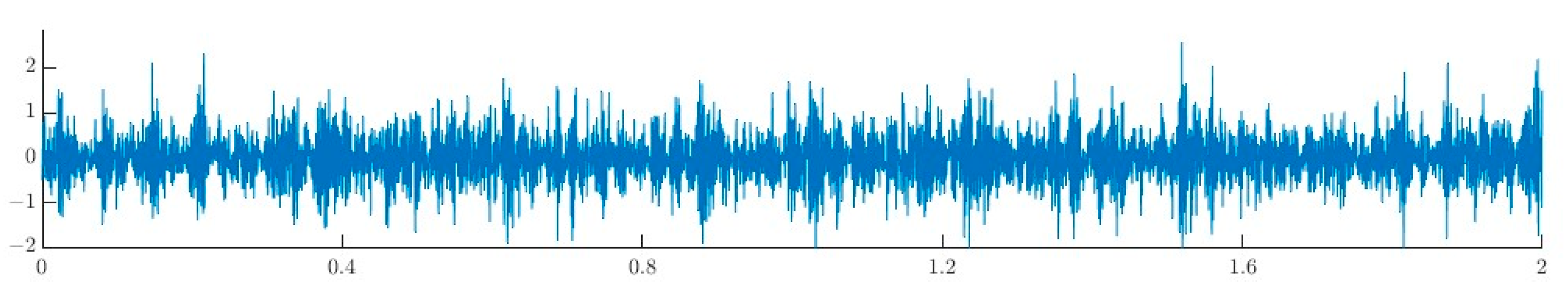
The sampling frequency of the signal is set to 16 kHz. Due to the large noise of the vibration signal, the overall signal-to-noise ratio of the signal is low; in order to ensure that the signal-to-noise ratio of the simulated signal model is −13, a Gaussian white noise signal with a signal-to-noise ratio of 0 is added to the signal. The time-domain signal is shown in
Figure 2, and it can be seen that the time-domain waveform signal is completely submerged after adding the noise.
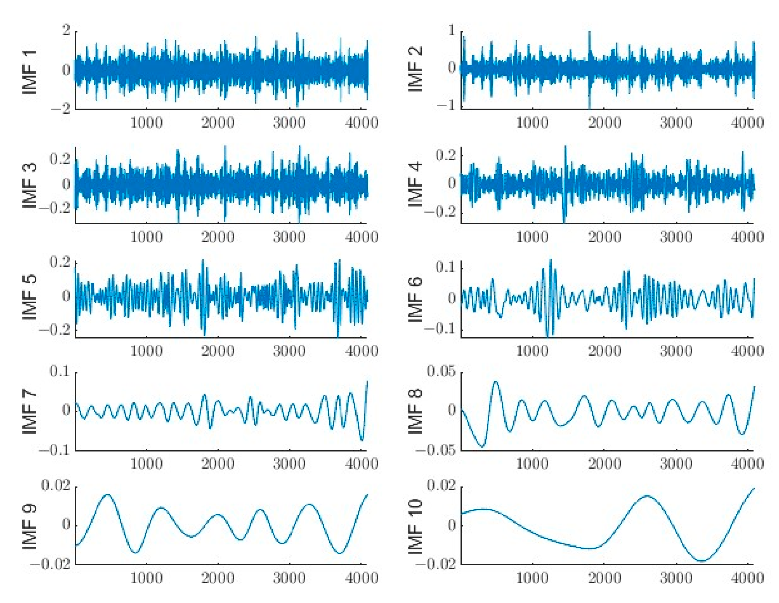
Noise-containing analog signals are individually decomposed using the EMD, EEMD, CEEMD, CEEMDAN, and modified CEEMDAN methods with the standard deviation of the added noise set to 0.2 and the number of loops to 100 for EEMD, CEEMD, CEEMDAN, and modified CEEMDAN. The decomposed IMFs of each order are shown in
Figure 3.
Through the decomposition of each order’s IMF, it is evident that the first six-order components possess greater information and exhibit more complex signal characteristics. To identify the high noise components for subsequent noise reduction, this study analyzes the similarity and correlation between the original signal, each IMF component, and among the IMF signals. The analysis focuses on metrics such as cross-correlation coefficient, kurtosis, and sample entropy values. Specifically, the cross-correlation coefficient, kurtosis, and sample entropy values are calculated for each order of IMF. The resulting values for the first six orders are presented in
Table 1. This table provides a comprehensive overview of the cross-correlation coefficients, kurtosis values, and sample entropy for each IMF component. The purpose of this analysis is to determine the components with higher noise content, enabling effective selection for the subsequent noise reduction process. By evaluating these metrics, the study gains insights into the characteristics and relationships among the IMF components and the original signal.
In the first six orders of IMF components, the overall number of cross-correlation coefficients is at a low level, indicating that the signal has been decomposed relatively well. After decomposition, the IMF with higher energy reflects the true extent of the vibration signal more accurately. Based on the classification criterion, the components can be categorized as spurious or valid components. The criterion involves comparing each IMF signal with the original data and calculating their correlation coefficient. The highest correlation coefficient is identified, and a threshold is set at one-tenth of this maximum correlation coefficient. IMF components with correlation coefficients below this threshold are considered spurious components, while those above the threshold are considered valid components [
36]. For the EMD method, the valid components are IMF1–IMF3. For the EEMD method, the valid components are IMF1–IMF3. For the CEEMD method, the valid components are IMF1–IMF3 and IMF5. In the case of the improved CEEMDAN method, the valid components are IMF1–IMF5. By comparing the results obtained from EMD, EEMD, and CEEMD, it is observed that the improved CEEMDAN decomposition produces more valid components and fewer spurious components. In the EMD decomposition method, mode mixing is a problem observed in components IMF2–IMF6, where they influence each other and are difficult to identify distinctly. However, the improved CEEMDAN decomposition effectively resolves the issue of mode mixing in the obtained components. The improved CEEMDAN method has the highest overall kurtosis level after decomposition, indicating the inclusion of relatively more effective signal components. The components with the top two kurtosis values are IMF4 and IMF5, while the overall kurtosis value of CEEMDAN is lower than that of the improved CEEMDAN algorithm, whose top two kurtosis-value components are IMF3 and IMF5. These components are analyzed by amplitude spectra and power spectra, respectively, as shown in
Figure 4 and
Figure 5.
It can be seen through the magnitude spectrum and power spectrum that the IMF3 after CEEDMAN decomposition has a higher magnitude in the interval of 0–4000 Hz, with worse overall concentration; IMF5 has a higher magnitude in the interval of 0–1000 Hz, with better overall concentration. While IMF4 after the decomposition of the improved algorithm has a high amplitude in the interval of 0–2000 Hz with a good overall concentration, IMF5 has a high amplitude in the interval of 0–1000 Hz with a high overall concentration. Overall, the amplitude concentration and energy concentration of the highest crag IMF of the improved algorithm are better than that of CEEMDAN, and although there are a large number of noise signals, the overall spectral characteristics of the improved algorithm after decomposition are obvious, and the interference frequency is better suppressed, which is conducive to the further identification of fault characteristics. Through the analysis above, it can be seen that the improved CEEMDAN algorithm can decompose the signal more effectively than the other methods of adaptive decomposition, and at the same time reduce the false components and improve the decomposition accuracy.
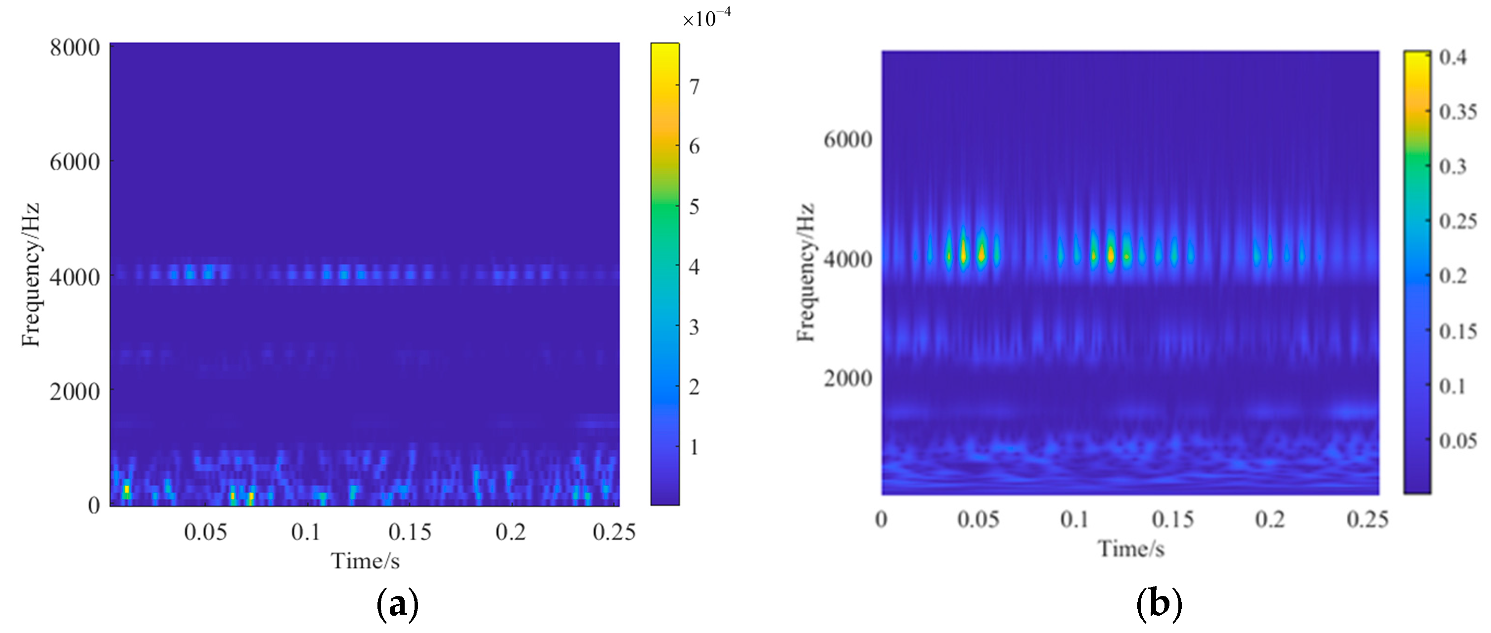
In order to further validate the performance of the proposed improved CEEMDAN algorithm with SVD joint noise reduction, further noise reduction is carried out on all orders of IMFs of the simulation signals extracted from combine harvester assembly quality problems using the improved CEEMDAN method. At the same time, to visualize the effect of noise reduction in the proposed method in this paper, the time–frequency diagrams of the original signal without noise, the original signal with noise, the original signal with direct noise reduction, and the original signal with CEEMDAN decomposition and then noise reduction are made by using the STFT and CWT methods. The proposed improved SVD noise reduction singular value threshold screening method is used, and the preset thresholds in Equation (25) are set to 0.2 to reduce the IMF containing more noise after the improved CEEMDAN decomposition; the signal is then reconstructed. To quantitatively evaluate the noise reduction effect of different methods on the signals, the signal-to-noise ratio (SNR) index (Equation (27)) is introduced to compare the noise reduction effect of various methods, and the calculation results are shown in
Table 2.
where:
is the sum of the effective power of the signal after noise reduction;
is the sum of the effective power of the original signal.
From
Figure 6, it can be seen that after adding the noise signal with higher intensity, the original signal is completely covered by the noise signal, and no matter if the time–frequency diagrams are plotted using STFT or CWT methods, the regular original signal cannot be recognized in
Figure 6c,d, as shown in
Figure 6a,b.
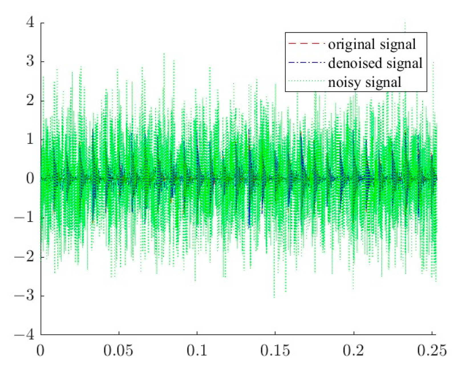
To provide a clearer and more intuitive assessment of the effectiveness of the joint noise reduction method, the figure below illustrates the time-domain graphs of the following signals: the noise-free test signal, the original signal containing noise, and the reconstructed signal obtained using the noise reduction method proposed in this paper. The graph clearly demonstrates the notable improvement achieved in reducing noise through the application of the proposed method.
From
Table 2, it can be seen that before the noise reduction process, the signal-to-noise ratio of the original signal after adding random white noise is −12.9989 dB; at this time, the signal is seriously distorted. By comparing, it can be seen that using Improved CEEMDAN denoising alone and using SVD denoising alone have certain denoising effects, with an improvement in SNR value. However, compared with the joint denoising of Improved CEEMDAN-SVD, the latter shows a significant increase in signal-to-noise ratio, reaching 0.9957 dB. This indicates that the joint denoising approach outperforms the individual denoising methods. From
Figure 7, it can be seen that the feature signals around 4000 Hz are better extracted, but there is some noise retained near 2500 Hz and above 6000 Hz that is not filtered out. It shows that the SVD method alone cannot filter out the strong noise, and other methods need to be used to assist the analysis.
Figure 8 shows the time–frequency diagram of the reconstructed noisy original signal after the improved CEEMDAN decomposition and SVD threshold noise reduction for each IMF, and it can be seen that the overall noise level of the signal after CEEMDAN decomposition and SVD threshold noise reduction for each IMF is reduced compared with the case in which the SVD threshold noise reduction is directly applied without CEEMDAN decomposition. The calculated correlation coefficient between the original signal and the denoised reconstruction is 0.8957. Combined with
Figure 8, it can be seen that although the original signal is somewhat distorted, it is generally well preserved. This indicates that the proposed method effectively reduces the impact of strong noise signals on the original signal.
To provide a clearer and more intuitive assessment of the effectiveness of the joint noise reduction method,
Figure 9 illustrates the time-domain graphs of the following signals: the noise-free test signal, the original signal containing noise, and the reconstructed signal obtained using the noise reduction method proposed in this paper. The graph clearly demonstrates the notable improvement achieved in reducing noise through the application of the proposed method.
4. Test Signal Analysis
The results of the simulation signal in the previous section verified the effectiveness of the method; the following experiment will be through the combined harvester bearing failure test data as an example to verify the effectiveness of the method proposed in this paper. The choice to adjust the combine harvester pulley to a non-tensioned state to simulate the bearing failure problem, the use of acceleration sensors to measure the vibration signal, a sampling frequency of 2 kHz, and an engine speed of 1000 r/min were established in the experiment. The simulation reduces the actual industrial site, divided into eight measurement points for the collection of vibration data. The sensor mounting position is shown in
Figure 10 and
Figure 11. This paper adopts the data in the fan bearing seat in the third measurement point as a verification of the validity of the test data of the proposed method; the raw data are shown in
Figure 12.
The improved CEEMDAN is used to decompose the test signal, and the decomposition results of each order of IMF are shown in
Figure 13. The kurtosis and sample entropy of each order of IMF are calculated separately, and the top six order values are listed as shown in
Table 3.
Table 3 shows that in the decomposed IMFs, the improved CEEMDAN has relatively lower sample entropy values compared with EMD, EEMD, CEEMD, and CEEMDAN. CEEMDAN has a relatively low sample entropy value compared with EMD, CEEMD, and CEEMDAN. Higher sample entropy values indicate higher complexity in the signal sequence. Therefore, the improved CEEMDAN decomposition can effectively decompose the signal while maintaining a higher decomposition accuracy. This is advantageous for the further denoising analysis of the signal. From
Table 3, it can be seen that for the test signals, the improved CEEMDAN decomposition has the largest kurtosis values for IMF2 and IMF4; therefore, it can be assumed that IMF2 and IMF4 contain more effective signals.
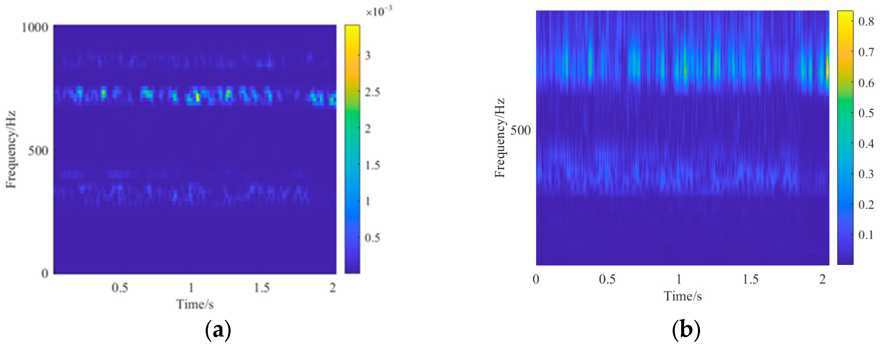
Figure 14 and
Figure 15 show the original test signal, the STFT and the CWT after the SVD noise reduction technique, respectively. For the combined harvester test signal, the method proposed in this paper was used for noise reduction. After joint denoising, the time–frequency analysis of the reconstructed combined harvester test signal was performed using STFT and CWT, as shown in
Figure 16.
Figure 16 displays the time–frequency plot of the combine harvester test signal after joint noise reduction and reconstruction. It can be observed that after joint noise reduction, the overall noise level of the signal is significantly reduced compared to the untreated experimental signal. To more intuitively see the noise reduction effect of various methods, the SNR is calculated to quantify the noise reduction effect, and the calculation results are shown in
Table 4. From the comparison of SNR values in
Table 4, it can be observed that for the combined harvester test signals, using the improved CEEMDAN denoising method alone and using the SVD denoising method alone result in some improvement in SNR. However, compared with the joint denoising approach of improved CEEMDAN-SVD, the latter shows a more significant improvement in SNR. This indicates that the proposed denoising technique is suitable for processing the vibration signals of combined harvester experiments and exhibits a good denoising performance.


