A Simulation-Based Approach to Evaluate the Performance of Automated Surveillance Camera Systems for Smart Cities

Abstract

A surveillance camera is the typical device that makes up a surveillance camera system in a modern city. It will still be a representative surveillance unit in future scenarios such as in smart cities. Furthermore, as the demand for public safety increases, a massive number of surveillance cameras will be in use in the future, and an automated system that controls surveillance cameras intelligently will also be required. Meanwhile, installing a surveillance system without any verification system might not be cost-effective, so a simulation that evaluates the system’s performance is required in advance. For this reason, we introduce how to simulate a surveillance area and evaluate surveillance performance in this paper to assess a surveillance system consisting of large amounts of surveillance cameras. Our simulator defined the surveillance area as a pair of two-dimensional planes, which depend on various camera-related configurations. Both surveillance areas are used to determine if the moving object belongs to the coverage of a surveillance camera. In addition, our simulator adopts several performance indices to evaluate a surveillance camera system in terms of target detection and quality. The simulation study provides comprehensive results on how various components of the surveillance system affect the performance of the surveillance system, leading to the conclusion that building a sophisticated scheme to control a large number of surveillance cameras can provide a cost-effective and reliable surveillance system for smart cities.

1. Introduction

One of the main goals of a smart city is to provide public safety to its citizens, and to achieve this goal, the city should establish a system that safeguards citizens from diverse threats. Surveillance camera operation systems such as CCTV (Closed Circuit Television) systems have already been established as a representative means of providing public safety in modern cities, but they are generally limited to simple crime prevention functions based on collections of evidence images. However, as intelligent surveillance cameras are equipped with advanced image processing systems based on deep learning technology, it is expected that surveillance camera operation systems will be able to more actively maintain urban security, and this requires a solution that can effectively operate a large number of surveillance cameras.

Figure 1 illustrates the functionality of the surveillance camera system under consideration in this paper. The system performs the functions of detecting targets in typical situations that threaten public safety, such as crime scenes, safety incidents, etc., and tracking infectious agents to protect citizens from emerging threats, such as epidemics. These types of situations all have origins in or are related to human behavior, which means that to prevent problems that threaten public safety in advance or to take appropriate follow-up actions, it is necessary to enhance the evidence-gathering capabilities of surveillance cameras. For this purpose, footage recorded both before and after the event occurs is required. Therefore, surveillance cameras need to seamlessly track and detect objects such as moving pedestrians or vehicles.

To realize the above scenario for public safety services, a precise calculation of the appropriate number and density of surveillance cameras, as well as the technical characteristics of the cameras, is required in advance, taking into account the features of the area and the object to be detected in the real world.

Meanwhile, due to the development of deep learning and image processing technology, the technology to recognize specific objects or situations through surveillance cameras has already reached a high level. Still, existing research on real-time surveillance camera operation systems has only considered a few CCTV cameras or has focused on the efficient placement of cameras. The application environment is limited to indoor or building interior spaces. It is challenging to design a system that operates many surveillance cameras in real time because there is no established method to evaluate the performance of a wide range of surveillance cameras with different physical characteristics.

For this reason, in this paper, as part of a digital twin world that mimics the real world, as shown in Figure 1, we implement a system-level simulator by modeling the surveillance performance of surveillance cameras, detection targets, and the local environment and devise several performance metrics to measure the detection performance and quality of the system to evaluate the performance of the system according to the physical characteristics of surveillance cameras.

That is, we aim to evaluate a surveillance system which consists of a vast number of surveillance cameras. The surveillance area is determined by two-dimensional planes (horizontal and vertical), indicating whether the target object falls within the surveillance camera’s coverage. The surveillance resolution is represented by the precision level shown on the display, which shows the target’s length per pixel in both the horizontal and vertical aspects. To determine the two surveillance indices, we consider several factors, such as the installed location, viewing angle, sensor format, focal length, and more.

Our simulation approach aims to assess the surveillance system’s performance in various scenarios to determine its effectiveness in detecting and tracking criminal activities. We propose a simulation model that considers different factors such as the number of cameras, their locations, and the type of target objects. Our model can evaluate the surveillance system’s performance based on the number of targets detected and the accuracy of target tracking.

The simulation results can provide valuable insights into the surveillance system’s performance to optimize the system’s design and improve its effectiveness. We can identify the weaknesses and strengths of the surveillance system and make necessary improvements to ensure better public safety. Our simulation approach can assist in decision making for installing surveillance systems and can be used to evaluate different surveillance system designs.

In conclusion, the implementation of a proficient surveillance system holds paramount significance in ensuring public safety. Our simulation methodology offers invaluable perspectives into the system’s operational efficacy, facilitating the enhancement of its design and functionality. The simulation model proposed can be employed to assess various surveillance system blueprints and aid decision making pertaining to the installation of a surveillance system in a smart city.

We summarize the contribution of our simulation models or simulators towards the assessment and enhancement of surveillance system performance below:

• Our simulation models offer a viable means of evaluating urban surveillance camera system performance, in line with the research objective of assessing system performance and identifying the factors that influence it.
• The model simulates a surveillance area using different camera-related configurations and evaluates the system’s performance based on target detection and quality.
• Through the definition of the surveillance area and consideration of various camera parameters, the simulation model ascertains whether moving objects fall within the surveillance camera’s scope of application, thereby providing insight into the system’s operational efficiency.
• A comprehensive insight into surveillance system performance is obtained from simulation results, enabling optimization of design and functionality. Moreover, the simulation approach can aid public safety improvements by supporting decision making regarding the installation of surveillance systems and the evaluation of various system designs.

Meanwhile, our simulations can be extended to model real-world surveillance camera system behavior, generating data in diverse environments and conditions. This feature facilitates data collection for learning artificial intelligence models and verifying their performance in varied settings. Additionally, data can be collected in a simulated environment, reducing the time and cost required for data collection in an actual environment.

The rest of this paper is organized as follows. In Section 2, previous research related to the topic of this study is provided. In Section 3, we introduce the modeling of a surveillance area and the target object to implement a surveillance camera system. This section will also determine whether a target object has been detected and introduce a performance index to evaluate the surveillance resolution. In Section 4, we analyze how various components of the surveillance camera system affect its performance using a simulation that we have implemented. Finally, we conclude our paper in Section 5.

2. Related Works

Modeling the coverage of surveillance cameras is essential for visual sensor applications and optimizing camera network placement. Various approaches have been proposed to address this challenge. A new approach called “HybVOR” is suggested for placing surveillance cameras using Voronoi-based 3D GIS techniques [1]. The goal is to achieve almost 100% coverage through three phases. One study proposed using imaging techniques to assist in the camera placement problem and to calculate camera coverage on a digitized 2D floor plan [2]. Another approach is a dynamic programming framework, which is introduced to optimize sensor coverage overlaps based on visual sensor parameters and the features of the monitored area [3]. This models the sensor coverage in a 2D space. In [4], an optimal policy is defined for solving the visual sensor coverage problem using a dynamic programming algorithm. It is compared to existing benchmarking placement optimization techniques to demonstrate its effectiveness in maximizing coverage for a set of predefined locations. The authors of [5] designed an approximation algorithm and an efficient heuristic algorithm based on pipage rounding to solve the maximum full-view target coverage problem in camera sensor networks, where each camera sensor has P working directions. In [6], the authors proposed integrating coverage inference and optimization methods into the existing GIS platform to promote various innovative applications in the camera planning area. An Alternate Global Greedy (AGG) algorithm was proposed in [7], a novel variant of the Global Greedy algorithm, to produce better coverage results. The experimental results show that the algorithms maximize coverage results with minimal overlap compared to existing greedy techniques. In [8], a camera network coverage model that considers obstacles and interesting areas of the environment is investigated and optimized by dynamic planning methods. The results show that this method can effectively improve the target capture rate of the network and observe the target from a better view. A study in [9] quantitatively evaluated the surveillance coverage of a CCTV system in an underground parking area and presented a full mathematical derivation for the resolution, which depends on the object’s location and orientation as well as the camera’s geometric model. Finally, the authors of [10] presented a distributed algorithm of perimeter surveillance that allows for the maintenance of total coverage in heterogeneous camera networks. This approach ensures maximum coverage with a minimum number of cameras.

In the field of video surveillance, it is important to evaluate the performance of surveillance camera systems. To do this, various methods and measures have been proposed. These include evaluating the reliability and effectiveness of video content analysis algorithms by assessing their segmentation, tracking, and event detection capabilities [11]. Additionally, new methods have been introduced to compare the performance of object detection algorithms in video sequences fairly [12]. Furthermore, the physical performance of surveillance cameras can be evaluated through measurements of spatial resolution, sensitivity, energy resolution, and image quality [13]. Regularly evaluating and documenting the performance of video surveillance systems is crucial to measure advancements and improve the efficiency and accuracy of these systems [14].

Various fields have conducted extensive research on the evaluation of surveillance camera systems. In [15], a dual-camera real-time video surveillance system could achieve accurate statistical inference, automatic control parameter adjustment, and precise limit quantification by carefully selecting system modules and analyzing the impact of tuning parameters. Another work [16] proposes a quantitative approach to evaluate the efficacy of CCTV coverage, where the surveillance resolution is determined by object positions and orientations. Furthermore, Bosch Corporate Research introduced a real-time video surveillance system that prioritizes robustness in its design [17]. This paper also presented quality measures for a common data set named PETS. Moreover, a set of objective, scientific evaluation indexes for user requirements of highway video surveillance networking systems were studied in [18]. These indexes were utilized to evaluate the performance of a developed video surveillance networking system and optimize its efficiency for real-time surveillance. Finally, study [19] suggests that analyzing the performance of a surveillance camera network system with an image recognition server based on the frame discard rate and server utilization can help ensure the efficient operation of evolving surveillance camera networks. The resulting analysis will be valuable for optimizing camera network systems.

Meanwhile, recent research has revealed that surveillance camera systems, such as CCTV, may not solely be employed for the purposes of preventing criminal activities, but they are also a crucial tool in resolving a multitude of issues, including traffic control, managing epidemics and disasters, and maintaining facilities.

In [20], the proposed PSI-CNN architecture improves face recognition performance by extracting untrained feature maps across multiple image resolutions, allowing the network to learn scale-independent information and outperforming the VGG face model in terms of accuracy. Paper [21] introduces a real-time ITS that uses video imaging and deep learning to detect vehicles driving the wrong way. The system achieves a 91.98% accuracy in detection by combining YOLOv3, Kalman filtering, and an “entry-exit” algorithm. Study [22] uses CCTV cameras in embedded systems to monitor traffic. A lightweight CNN and the SORT algorithm enable real-time processing for vehicle detection and tracking. Labels are generated in an unsupervised manner, improving traffic estimation accuracy. In study [23], an AI-powered system uses CCTV cameras to monitor social distancing and identify high-risk zones for infection. The proposed system outperforms traditional methods in person detection and offers a risk assessment scheme. In [24], a new model is proposed that achieves better action recognition and real-time capability, making it suitable for low-cost GPU-based embedded systems. This study suggests an algorithm that uses a deep learning model to improve vehicle license plate recognition in CCTV images. A deep learning model was created for detecting road abnormalities and preventing accidents in [25]. It utilized FFmpeg to extract accident images and identified collision types using the YOLO algorithm. The service included a car accident and road obstacle detection model, warning notifications, and photo capture. The authors of [26] dealt with detecting weapon problems in CCTV surveillance videos. Here, advances in computer vision and object detection led to a real-time system using a high-performance GPU and optimized implementation for improved speed and accuracy. Digital twin technology can aid in disaster safety management of underground utility tunnels. The study in [27] compared two methods for estimating depth using a single CCTV camera: the coordinate system conversion method and the DenseDepth transfer learning method. The coordinate system conversion method was found to be more suitable for accurate depth estimation. Manually detecting sewer defects can be a time-consuming and ineffective process. Therefore, an accurate and automated detection method is necessary. In a previous study [28], the authors suggested the utilization of YOLOv4 with the SPP module and the DIoU loss function to enhance detection and classification accuracy.

3. Simulation Model for Surveillance Systems

In this section, we introduce a simulation model for a surveillance system designed to monitor a specific location and detect target objects. To provide a better understanding of our implemented system, we have included Figure 2a, which offers a detailed visualization of the model. To enhance clarity, viewers can watch a simulation demonstration at https://youtu.be/-InCVtvPu3M (accessed on 6 August 2023).

The model follows a systematic approach, starting with the surveillance camera area modeling. Subsequently, the targets, which could be pedestrians or other monitored entities, are modeled. We also consider various factors such as roads and intersections while modeling the local environment. Finally, we assess the surveillance system’s performance to determine its performance.

3.1. The Overview of Simulator Structure

Our simulator was primarily coded using the C# programming language on the Windows 10 operating system. We utilized MATLAB only for visualization purposes. The complete source code is available in the GitHub repository at https://github.com/0BoOKim/Surveillance_System_Revision (accessed on 6 August 2023).

The fundamental approach taken to implement our system-level simulator involves defining classes that configure the surveillance camera, pedestrians, and the environment. Each class is responsible for generating a predetermined number of instances of surveillance cameras and pedestrians. These entities are then placed on an environment created through the employment of the environment class. This holistic approach enables conducting a comprehensive, system-level simulation of a surveillance camera system. 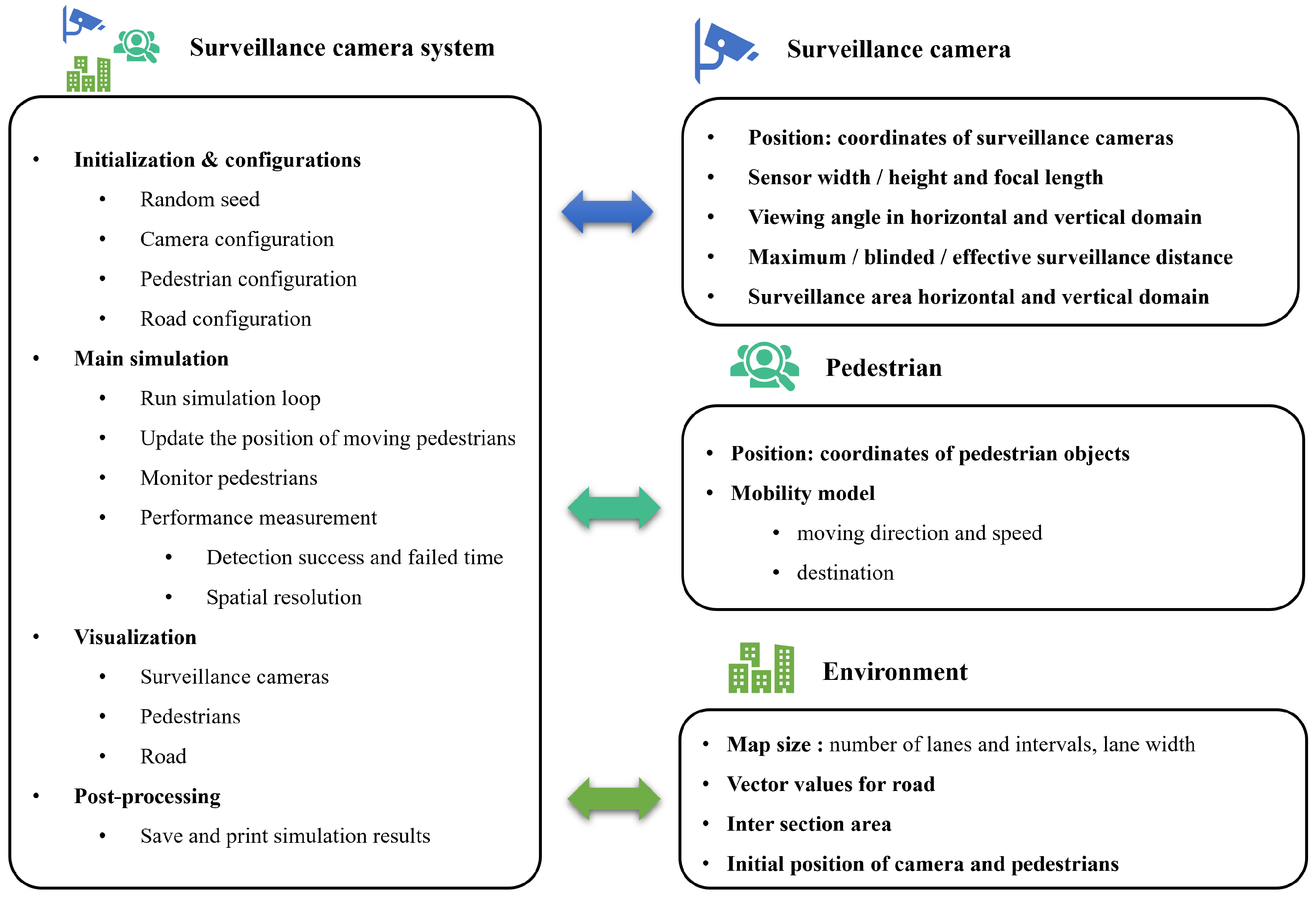Figure 3 illustrates the architecture of the developed simulation, demonstrating its core structure and components. The main simulation revolves around the utilization of classes that meticulously define the attributes and functionalities of key elements, namely surveillance cameras, pedestrians, and the environment.

To start, the Surveillance Camera Class plays a pivotal role in the simulation. This class encapsulates the intricate details of surveillance cameras, encompassing their crucial characteristics and behaviors:

• The Position property indicates the precise coordinates of each surveillance camera within the simulated environment.
• Properties like Sensor Width, Sensor Height, and Focal Length contribute to configuring the camera’s sensor, dictating its capture dimensions and focus capabilities.
• Viewing Angles in both Horizontal and Vertical domains are also integral properties, determining the extent of the camera’s observable field.
• The trio of Maximum Surveillance Distance, Blinded Surveillance Distance, and Effective Surveillance Distance properties together outline the range within which the camera operates, accounting for its maximum reach, potential obstructions, and optimal monitoring capability.
• Lastly, the class defines the Surveillance Area in the Horizontal and Vertical domains, reflecting the actual coverage area based on sensor dimensions, viewing angles, and distances.

Moving on, the Pedestrian Class is another crucial element of the simulation:

• Within this class, the Position property manages the specific coordinates of each pedestrian object in the environment.
• The class also incorporates a Mobility Model, encapsulating details like the pedestrian’s moving direction and speed as well as their intended destination.

Lastly, the Environment Class encapsulates foundational aspects of the simulated environment:

• It includes attributes like Map Size, which indicates the number of lanes, intervals, and the lane width, defining the scope and structure of the environment.
• Vector Values for Roads store critical information about the road network’s layout and characteristics.
• This class accounts for Intersection Areas, pivotal sections where roads cross each other.
• Additionally, it encompasses details about the Initial Positions of Cameras and Pedestrians, setting the stage for the simulation’s starting conditions.

Collectively, these classes constitute the backbone of the simulation, as described below, enabling the accurate representation and interaction of surveillance cameras, pedestrians, and the environment. By utilizing these meticulously designed classes, the simulation effectively mirrors physical world scenarios and facilitates comprehensive analysis.

• Initialization and Configuration: To ensure consistent randomness, it is imperative to set the random seed. This should be done prior to configuring the surveillance cameras, which involves determining their positions and properties. Additionally, parameters for pedestrians, including their initial positions and behavior, should be set up. Finally, the road layout should be configured, defining lanes, intersections, and dimensions.
• Main Simulation: The execution of the simulation loop is the core of the simulator, and as such, it must be executed seamlessly. Continuously updating the positions of moving pedestrians based on their behavior is necessary. It is also imperative to monitor the pedestrians’ interactions with the environment and cameras. The system’s performance should be measured by tracking detection successes, failures, and spatial resolution.
• Visualization: Visualizing the surveillance cameras’ coverage areas and positions is crucial, as is displaying the movements of pedestrians within the simulation environment. The road layout should be rendered, showing the lanes and intersections.
• Post-Processing: Saving and storing the simulation results, which include data on pedestrian paths, camera detections, and system performance, are essential. Furthermore, options to print or export the simulation outcomes for further analysis and reporting should be provided.

3.2. Surveillance Area

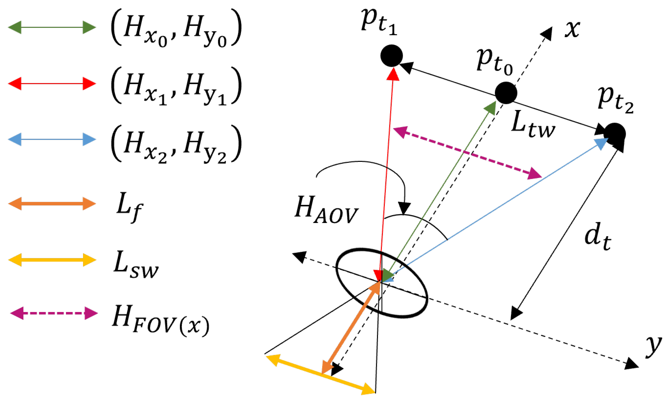
Figure 2b depicts the various parameters of an image sensor (shown in small rectangles), an optic lens (shown in ellipses), and a target object (shown in large rectangles). Initially, we assume that the center of the optic lens is located at (0,0) and the plane of the target object is accurately parallel with the image plane (or the optic lens). Then, we consider the level of rotation of the optic lens and the image plane (i.e., the viewing angle of the camera) to calculate the surveillance area in the coordinate system.

As shown in Figure 2b, a camera’s surveillance area in horizontal aspects lies within the two borderlines represented by $(H_{x_1},H_{y_1})$ and $(H_{x_2},H_{y_2})$, respectively. Another line represented by $(H_{x_0},H_{y_0})$ goes through the surveillance area’s center, which divides the surveillance area in half and is also utilized to determine if the target belongs to the surveillance area. Equations (1) and (2) define these three lines: the function of variable x for the distance from the optic lens to the target, where $H_{FOV}\left(x\right)$ is the FOV (Field of View) for variable x and ${\theta }_h$ is the viewing angle of the camera. Here, the FOV is a well-known factor defined as $H_{FOV}\left(x\right)=x\times \frac{L_{sw}}{L_f}$, and $L_{sw}$ and $L_f$ are the width of the image sensor and the focal length, respectively. A further elaboration of Equations (1) and (2) from a geometrical perspective can be found within the confines of Appendix A of this paper.

$$H_{x_i}=\left\{\begin{array}{cc}xcos{\theta }_h\hfill & i=0\hfill \\ xcos{\theta }_h-\frac{1}{2}{H}_{FOV}\left(x\right)sin{\theta }_h\hfill & i=1\hfill \\ xcos{\theta }_h+\frac{1}{2}{H}_{FOV}\left(x\right)sin{\theta }_h\hfill & i=2\hfill \end{array}\right.$$

(1)

$$H_{y_i}=\left\{\begin{array}{cc}xsin{\theta }_h\hfill & i=0\hfill \\ xsin{\theta }_h+\frac{1}{2}{H}_{FOV}\left(x\right)cos{\theta }_h\hfill & i=1\hfill \\ xsin{\theta }_h-\frac{1}{2}{H}_{FOV}\left(x\right)cos{\theta }_h\hfill & i=2\hfill \end{array}\right.$$

(2)

In the vertical aspect, the surveillance area is also calculated by (3) and (4), which are similar to (1) and (2); however, several factors, such as the FOV $H_{FOV}\left(x\right)$ and the viewing angle ${\theta }_h$, should be substituted. That is, $H_{FOV}\left(x\right)$ is replaced with $V_{FOV}\left(x\right)$, defined as $x\times \frac{L_{sh}}{L_f}$, and ${\theta }_v$ is used for the viewing angle in the vertical aspect instead of ${\theta }_h$.

$$V_{x_i}=\left\{\begin{array}{cc}xcos{\theta }_v\hfill & i=0\hfill \\ xcos{\theta }_v-\frac{1}{2}{V}_{FOV}\left(x\right)sin{\theta }_v\hfill & i=1\hfill \\ xcos{\theta }_v+\frac{1}{2}{V}_{FOV}\left(x\right)sin{\theta }_v\hfill & i=2\hfill \end{array}\right.$$

(3)

$$V_{z_i}=\left\{\begin{array}{cc}xsin{\theta }_v\hfill & i=0\hfill \\ xsin{\theta }_v+\frac{1}{2}{V}_{FOV}\left(x\right)cos{\theta }_v\hfill & i=1\hfill \\ xsin{\theta }_v-\frac{1}{2}{V}_{FOV}\left(x\right)cos{\theta }_v\hfill & i=2\hfill \end{array}\right.$$

(4)

Lastly, since we assumed that the center of the optic lens was located at (0, 0), the surveillance area of the coordinate system should be corrected to the original coordinates by (5).

$$\begin{array}{cc}\hfill \overline{H_{x_i}}& =H_{x_i}+x_o\hfill \\ \hfill \overline{H_{y_i}}& =H_{y_i}+y_o\hfill \\ \hfill \overline{V_{x_i}}& =V_{x_i}+x_o\hfill \\ \hfill \overline{V_{z_i}}& =V_{z_i}+L_{ih}\hfill \end{array}$$

(5)

The next step is to determine the effective surveillance distance of the camera, as depicted in Figure 4. The effective surveillance distance of the camera is defined by (6), which is determined by taking into account the difference between the camera’s maximum surveillance distance, denoted by $D_{max}$, and its distance to the blind zone, as represented by $D_{bz}$.

$$D_{eff}=D_{max}-D_{bz}$$

(6)

$$D_{max}=(L_{ih}-L_{th}^{max})\times tan\left(\frac{\pi -V_{AOV}}{2}-v_v\right)$$

(7)

As defined in (7), the camera’s maximum surveillance distance, denoted by $D_{max}$, is calculated on the basis of the height of the target object that the camera can detect. Here, $L_{ih}$ denotes the installation height of the surveillance camera, $L_{th}^{max}$ denotes the maximum height of the target object, $V_{AOV}=arctan(L_{sh}/2L_f)$ refers to the angle of view of the camera, and $V_v$ represents the viewing angle of the camera.

$$D_{bz}=L_{ih}\times tan\left(\frac{\pi +V_{AOV}}{2}-v_v\right)$$

(8)

Finally, (8) is the means by which one can determine the camera’s distance to the blind zone. The distance to the blind zone is determined by the camera’s installation height, the camera’s angle, and the camera’s angle of view in the vertical domain.

3.3. Target Object and Target Detection

In this section, we first describe the modeling of the target object and then the way to determine if the target object is located in the surveillance area in the horizontal domain. First, we define the target object as the three points $p_{t_0}$, $p_{t_1}$, and $p_{t_2}$ for the horizontal aspects. The point $p_{t_0}$ is the center of the target, and $p_{t_1}$ and $p_{t_2}$ are the points that either the shortest and the longest point, respectively, depending on the distance from the optic lens. Since, in most cases, the plane of the target, represented by the large rectangle in Figure 2b, is not parallel to the optic lens and the image plane, we consider the angle of the rotation of the target plane ${\theta }_t$ to determine if the target belongs to the surveillance area. In other words, the target is located in the surveillance area only if all the points represented in (9) are located within the surveillance area.

$$p_{t_i}(x,y)=\left\{\begin{array}{cc}(x_t-x_o,y_t-y_o)\hfill & i=0\hfill \\ (-\frac{L_{tw}}{2}sin{\theta }_t,\frac{L_{tw}}{2}cos{\theta }_t)+p_{t_0}(x,y)\hfill & i=1\hfill \\ (\frac{L_{tw}}{2}sin{\theta }_t,-\frac{L_{tw}}{2}cos{\theta }_t)+p_{t_0}(x,y)\hfill & i=2\hfill \end{array}\right.$$

(9)

To determine whether a target object lies within a designated surveillance area, it is imperative to preliminarily establish whether the object is located within the efficient surveillance distance $D_{eff}$, as described in Section 3.2. In the event that the object is indeed situated within $D_{eff}$, the procedure is executed as described as follows.

The key factor for target detection is the AOV (angle of view), a well-known formula like the FOV, and is defined as $H_{AOV}=2arctan(L_{sw}/2L_f)$. If positions $p_{t_1}$, $p_{t_2}$, and $p_{t_3}$ are in the surveillance area, the angles of $p_{t_1}$, $p_{t_2}$, and $p_{t_3}$ must be within the angular extent of $H_{AOV}$, which can determined by (10).

$$\frac{P_H•P_T}{\parallel P_H\parallel \times \parallel P_T\parallel }\le cos\left(\frac{H_{AOV}}{2}\right)$$

(10)

where $P_H$ is any coordinate in $(H_{x_0},H_{y_0})$ except (0, 0) and $P_T$ is one of the coordinates of $p_{t_i}$. That is, the target is in the surveillance area if the angle between the centerline of the surveillance area and the line from the origin and the target point is smaller than the AOV. Similar to the procedure to calculate the horizontal surveillance area, the discriminating procedure for target detection is repeated in terms of the vertical surveillance area.

3.4. Surveillance Resolution

In this section, we introduce how to measure the surveillance resolution of the target object in the simulation. The first step to calculate the target’s resolution is the sampling distance calculation of $S{D}_{h_i}$ and $S{D}_{v_i}$, which are the sampling distances for horizontal and vertical aspects, respectively. (The sampling distance is the distance between the centers of two adjacent pixels in an image, as represented as the length per pixel, which is measured based on the distance from the optic lens to the target object, the width of the image sensor, the focal length, and the number of pixels on the image sensor.) Then, we represent the sampling distance in two ways based on the value of the sampling distance considering the minimum and maximum distance from the optic lens to the target.

First, the sampling distances $S{D}_{h_i}$ and $S{D}_{v_i}$ in the horizontal and vertical aspect are calculated by (11) and (12).

$$\begin{array}{c}\hfill S{D}_{h_i}=\frac{L_{sw}\times d_i^h}{L_f\times i{m}_w}\end{array}$$

(11)

$$\begin{array}{c}\hfill S{D}_{v_i}=\frac{L_{sh}\times d_i^v}{L_f\times i{m}_h}\end{array}$$

(12)

where $d_i^h$ is the distance from the optic lens to the target point $p_{t_i}$, and $i{m}_w$ is the number of pixels on the image sensors in the horizontal aspect. Similarly, $d_i^v$ and $i{m}_h$ are the distance from the optic lens to the target point and the number of pixels on the image sensors in the vertical domain. As mentioned in Section 3.3, since in most cases, any plane of the target object is not parallel with the image sensor and the optic lens, the sampling distance is not uniform on the target plane, so we can classify it into two types of the sampling distance, i.e., the minimum and maximum values. For example, in Figure 2b, the distance from the optic lens to $p_{t_2}$ is the shortest, so the sampling distance is the highest and $S{D}_{h_2}$ is the maximum sampling distance $S{D}_{h_i}^{max}$, whereas $S{D}_{h_1}$ is the minimum sampling distance of the target object.

As the sampling distance is available, the target object’s number of pixels in the horizontal and vertical aspect is determined using (13). Note that the surveillance resolution in the vertical aspect is also calculated similarly to the horizontal aspect.

$$\begin{array}{c}\hfill S{R}_i=P_{h_i}\times P_{v_i}\end{array}$$

(13)

$$\begin{array}{c}\hfill P_{h_i}=\frac{L_{tw}}{S{D}_{h_i}^{max}}\end{array}$$

(14)

$$\begin{array}{c}\hfill P_{v_i}=\frac{L_{th}}{S{D}_{v_i}^{max}}\end{array}$$

(15)

Herein, the surveillance resolution of target i is denoted by $S{R}_i$. It is determined by the product of the number of horizontal pixels $P_{h_i}$ and the number of vertical pixels $P_{v_i}$, as represented by (14) and (15), respectively. The quantity $P_{h_i}$ corresponds to the number of pixels that lie in the horizontal domain. It is computed as the ratio of the width $L_{tw}$ of the target to the maximum horizontal sampling distance, $S{D}_{h_i}^{max}$. Similarly, $P_{v_i}$ represents the number of pixels that fall in the vertical domain. It is calculated as the quotient of the height, $L_{th}$, of the target and the maximum vertical sampling distance, $S{D}_{v_i}^{max}$. Hence, it can be inferred that the surveillance resolution $S{R}_i$ is an indicator of the maximum number of pixels that can be used by the surveillance camera to represent a target that is modeled as a rectangle.

4. Simulation Study

4.1. Simulation Configurations

In the simulation configuration, as shown in

Table 1. Default configurations in simulation scenarios.

Category	Description	Value
Surveillance camera	number of surveillance cameras	10–500
	focal length (mm)	2.8
	sensor width (mm)	4.8
	sensor height (mm)	3.6
	image width in pixel (pixels)	1920
	image height in pixel (pixels)	1080
	viewing angle in horizontal domain (degree)	semi−random
	viewing angle in vertical domain (degree)	−45
	installation height (m)	5
	maximum target height (m)	3
Pedestrian	number of pedestrians	100
	width of pedestrians (m)	0.9
	height of pedestrians (m)	1.7
	moving speed of pedestrians (m/s)	1.7
	road width (m)	10
Road	road interval (m)	25
	number of road interval	5
Simulator	unit time (ms)	100
	simulation time (s)	600

, parameters can be assigned within four categories: the surveillance camera, the pedestrians, the road, and the simulator. Unless mentioned otherwise, the default values for each setting in the simulation are those listed in Table 1.

In addition, pedestrians commonly move along the road at an average walking speed of 1.7 m/s, targeting adjacent intersections as their destination, and when they reach their destination, they randomly select one of the adjacent intersections as their new destination. This process was repeated until the simulation ends. Cameras were placed randomly but constrained to be adjacent to the road. Similarly, the horizontal viewing angle of the cameras was randomized, but we constrained the camera’s viewing area to include the road.

The simulation evaluates the impact of the number of cameras (density); the number of pedestrians as target objects; the size, focal length, and resolution of the surveillance camera sensors; and the installation height of the cameras in terms of several performance metrics. For the performance evaluation, the key performance indicators are (i) detection success time $T_{suc}$, which is the average time taken for a pedestrian to be detected by at least one of the surveillance cameras, and detection failed time $T_{fail}$, which is the average time taken for a pedestrian not to be detected. This is further subdivided into two situations: (ii) when the pedestrian is out of the effective coverage area $T_{fail}^{out}$, and (iii) when the pedestrian is within the effective surveillance distance but the viewing angle of the surveillance camera is angled in the wrong direction $T_{fail}^{dir}$. Furthermore, to evaluate the surveillance quality of the monitored pedestrians, the surveillance resolution value described in Section 3.4 was measured every 100 ms. In each simulation, the values in the sample were obtained by taking the average of 10 iterations.

4.2. Effect of the Number of Surveillance Cameras

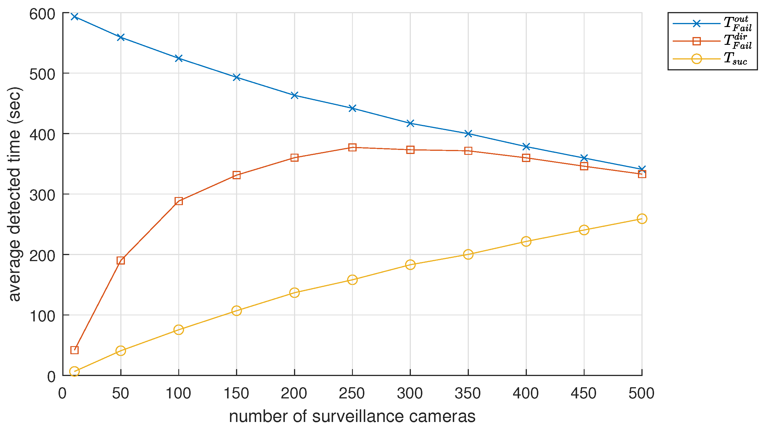
In this section, we evaluate how the number of surveillance cameras affects the performance of the surveillance system. Figure 5 shows the change in performance $T_{suc}$, $T_{fail}^{out}$, and $T_{fail}^{dir}$ as the number of surveillance cameras is increased from 10 to 500, with the number of pedestrians fixed at 10.

$T_{suc}$ refers to the duration of the successful detection of pedestrians within the coverage area, and $T_{suc}$ consistently increases from 6.6 to 259.0 s as the number of surveillance cameras is increased from 10 to 500. This indicates a positive correlation between the number of cameras and the successful detection time.

$T_{fail}^{out}$ refers to the duration of time for which the pedestrians are outside of the effective detection area. As the number of cameras increases from 10 to 500, the $T_{fail}^{out}$ values decrease from 593.4 to 340.1 s, indicating the improved performance of the surveillance system.

From this observation of $T_{suc}$ and $T_{fail}^{out}$, it is clear that pedestrians can be detected more frequently as the number of surveillance cameras increases. However, even when the number of cameras is increased from 10 to 500, which is 50 times the initial number, pedestrians are still not detected for 340 s, which represents 56% of the total simulated time of 600 s. This suggests that merely equating the number of cameras to increase the surveillance coverage could be inefficient in terms of cost and performance improvement.

The time for which pedestrians are within range but undetected due to incorrect camera directions is referred to as $T_{fail}^{dir}$. In Figure 5, as the number of surveillance cameras increased from 10 to 250, the values of $T_{fail}^{dir}$ increased from 41.8 to 377.1 s but ceased to increase when the number of cameras exceeded 260.

It is important to note that $T_{fail}^{dir}$ is a partial representation of $T_{fail}^{out}$, signifying that some pedestrians who were initially undetected could be detected with a proper camera direction. For instance, if there were 100 surveillance cameras, $T_{fail}^{out}$ and $T_{fail}^{dir}$ would be 524.5 s and 288.3 s, respectively. By correctly controlling the camera direction, the time it takes to detect pedestrians could be reduced by 288.3 s, a performance improvement of roughly 55%. In a separate scenario with 500 surveillance cameras, $T_{fail}^{out}$ and $T_{fail}^{dir}$ are 340.9 and 332.9 s, respectively. This suggests that controlling the camera orientation could decrease the duration that pedestrians went undetected for by 97.7%.

4.3. Effect of the Number of Pedestrians

In this subsection, we present the simulation outcomes that illustrate the correlation between the number of pedestrians and the efficacy of the surveillance system, as indicated by the detection time $T_{suc}$, out-of-range time $T_{fail}^{out}$, and direction error time $T_{fail}^{dir}$.

In the simulation scenario, the number of pedestrians observed ranged from 10 to 500, whereas the number of surveillance cameras deployed was 10, 100, 200, 300, 400, or 500.

As demonstrated in Figure 6a, the detected time $T_{suc}$ is shown across various numbers of surveillance cameras for multiple counts of pedestrians ranging from 10 to 500. Upon investigation, it was established that the detected time $T_{suc}$ exhibited similar values even as the number of pedestrians increased. This finding reaffirms the notion that the number or density of surveillance cameras serves as the primary influencer of performance in terms of $T_{suc}$, not the number of pedestrians.

To illustrate, the detected time ranged from 7.7 to 8.3 s, 182.1 to 183.7 s, and 253.5 to 258.4 s, respectively, when the number of surveillance cameras was 10, 300, and 500. Furthermore, it is important to note that the standard deviation values of the detected time were only 0.2, 0.7, and 1.3 s, respectively, when the number of surveillance cameras was 10, 300, and 500 respectively.

The results for the additional performance metrics, $T_{fail}^{out}$ and $T_{fail}^{dir}$, exhibit similarities. In Figure 6b,c, we present the out-of-range time $T_{fail}^{out}$ and the direction error time $T_{fail}^{dir}$ in relation to various numbers of surveillance cameras and multiple numbers of pedestrians ranging from 10 to 500.

For instance, when there were 10, 300, and 500 surveillance cameras, the out-of-range time ranged from 591.7 to 592.3 s, 416.3 to 417.2 s, and 341.6 to 346.5 s, respectively. Furthermore, the standard deviation values of the out-of-range time were only 0.2, 0.5, and 1.3 s, respectively, when there were 10, 300, and 500 surveillance cameras.

The direction error time was observed to range from 45.9 to 47.5 s, 371.6 to 373.8 s, and 332.2 to 338.4 s, respectively, when the surveillance camera count was 10, 300, and 500. The standard deviation values of the recorded time were only 0.5, 0.6, and 1.4 s, respectively, for the same surveillance camera counts.

In conclusion, it can be inferred that the number of pedestrians does not significantly influence the performance of the surveillance system in terms of $T_{suc}$, $T_{fail}^{out}$, and $T_{fail}^{dir}$. Therefore, for subsequent simulations in this paper, the number of pedestrians was fixed at 100, and its effect is no longer considered.

4.4. Effect of the Camera Sensor Dimension

In the present subsection, we have delved into the impact of the camera sensor size on surveillance camera system functioning. The dimensions of the sensors of surveillance cameras are conventionally $(L_{sw},L_{sh})$ = (3.2 mm, 2.4 mm), (4.8 mm, 3.6 mm), (5.76 mm, 4.29 mm), and (6.4 mm, 4.8 mm), horizontally and vertically. The average detection time performance $T_{suc}$ for various sensor sizes is illustrated in Figure 7a. Our observation reveals that with an increase in the number of cameras, $T_{suc}$ escalates roughly 72-fold from 0.22 s to 15.90 s for the smallest sensor size ($(L_{sw},L_{sh})$ = (3.2 mm, 2.4 mm)), but this was significantly lower in comparison to the increase from 8.15 s to 257.12 s for $(L_{sw},L_{sh})$ = (4.8 mm, 3.6 mm).

In essence, it is important to note that an increase in the density of surveillance cameras and the number of cameras deployed does not necessarily guarantee an improvement in performance, especially if the size of the camera’s sensor is small and the surveillance area is subsequently limited. This is due to the fact that the size of the sensor is directly proportional to the coverage area of each camera.

On the contrary, when the size of the camera sensor is at its largest, with dimensions of $(L_{sw},L_{sh})$ = (6.4 mm, 4.8 mm), there is a significant improvement in the average detection time, increasing from 56.57 s to 553.58 s. In other words, with the highest density of surveillance cameras, $N_{cam}$ = 500, a pedestrian can be detected 92% of the time.

Hence, it can be inferred that the coverage provided by every surveillance camera, covering a wider area owing to the larger sensor size, yields a noteworthy enhancement in the detection time $T_{suc}$. Consequently, this leads to more productive surveillance and an improved public safety service approach.

However, as depicted in Figure 7b, it is evident that the performance in terms of surveillance resolution per millisecond can potentially fall with larger camera sensor dimensions. For instance, the sensor with the most diminutive dimensions, $(L_{sw},L_{sh})$ = (3.2 mm, 2.4 mm), exhibits the lowest $T_{suc}$ performance. Nevertheless, the surveillance resolution per millisecond performance records an average of 242.65 kilopixels/ms.

Conversely, the $T_{suc}$ performance of the sensor with the highest values of $(L_{sw},L_{sh})$ = (6.4 mm, 4.8 mm) is superior. However, even when considering the highest surveillance resolution value per millisecond (i.e., 55.85 kilopixels/ms when $N_{cam}$ was 500), it only attains a quarter of the performance of $(L_{sw},L_{sh})$ = (3.2 mm, 2.4 mm).

In other words, if the surveillance resolution provided is inadequate for target identification or if a closer observation of the target is necessary, then configuring the system with a surveillance camera with a sensor size of $(L_{sw},L_{sh})$ = (6.4 mm, 4.8 mm) may not suffice.

In conclusion, when contemplating the trade-off between detection time and surveillance resolution per ms, and given that only one sensor needs to be mounted on the surveillance camera, it may be feasible to mount a sensor with $(L_{sw},L_{sh})$ = (4.8 mm, 3.6 mm), for which both performance metrics are moderate. However, suppose multiple sensors with different specifications can be installed on a single surveillance camera. In this case, it might be more effective to select the appropriate sensor in accordance with the requirements of detection time and surveillance resolution per ms.

4.5. Effect of the Focal Length

In this section, we demonstrate the impact of focal length on performance via simulation results. The experiments encompassed 2.8 mm, 3.6 mm, and 6.0 mm focal lengths.

Analogous to the sensor size, the focal length notably influences the detection area and quality.

In Figure 8a, the detection time, denoted as $T_{suc}$, was monitored while increasing the number of surveillance cameras with varying focal lengths. When considering a focal length of 2.8 mm, the smallest of the focal lengths studied, $T_{suc}$, exhibited an increase from 8.15 s to 257.12 s as the number of surveillance cameras increased. In the case of focal lengths of 3.6 mm and 6.0 mm, $T_{suc}$ demonstrated an increase from 1.18 s to 59.59 s and from 0.0 s to 7.96 s, respectively, as the number of surveillance cameras increased.

That is, similar to the impact of sensor size on performance, as highlighted in the preceding section, a noteworthy decrease in detection time performance is observed as the surveillance area diminishes with an increase in focal length.

In accordance with Figure 8b, the surveillance resolution per ms is depicted as we increase the quantity of surveillance cameras with varying focal lengths.

Upon utilizing the smallest focal length of 2.8 mm, an increase in surveillance resolution per ms performance is observed, escalating from 55.98 to 87.31 kilopixels/ms as the number of surveillance cameras increases.

Similarly, for a focal length of 3.6 mm, the surveillance resolution per ms increases from 131.77 to 146.15 kilopixels/ms as the number of surveillance cameras increases. In contrast, for the longest focal length of 6.0 mm, the surveillance resolution per ms exhibits a fluctuation between 559.90 and 576.45 kilopixels/ms as the number of surveillance cameras is heightened.

In a manner akin to the influence that sensor size wields on performance, as was discussed in the above section, it is noteworthy that a heightened focal length leads to a reduction in detection time owing to the decreased size of the surveillance area. It is, however, relevant to report that the surveillance resolution per millisecond may escalate by a factor of 10 or more.

4.6. Effect of the Camera Resolution

This section presents an analysis of the performance of surveillance cameras based on the number of cameras deployed with different resolutions. The resolutions considered in this analysis are 720 p, 1080 p, 1440 p, and 2160 p. The objective of this analysis is to determine the impact of camera resolution on detection time.

The results of this analysis are presented in Figure 9a, which illustrates the performance in terms of detection time $T_{suc}$. For instance, when the resolution is 720 p, the detection time increases from 8.0 s to 259.1 s as the number of surveillance cameras increases from 10 to 500. Similarly, for 1080 p resolution, as the number of surveillance cameras increases from 10 to 500, the detection time increases from 8.2 s to 257.1 s. At 1440 p resolution, the detection time increases from 8.4 s to 258.4 s, while at 2160 p resolution, the detection time increases from 8.1 s to 257.7 s. The detection time values are comparable regardless of the resolution in question, and the difference in the detection time among various resolutions only ranged from 0.1 to 1.3 s. That is, only the number of surveillance cameras was a dominant factor in this simulation study. This is because the resolution is not a mandatory configuration for the surveillance area.

In terms of measuring the quality of surveillance performance, the surveillance resolution per ms demonstrates a clear relationship with surveillance camera resolution. The performance of surveillance camera systems with different resolutions is displayed in Figure 9b, and the results indicate that as the number of surveillance cameras increases from 10 to 500, the surveillance resolution per ms increases from 24.79 to 38.78 kilopixels/ms at a resolution of 720 p.

When the resolution is increased to 1080 p, the surveillance resolution per ms increases from 55.98 to 87.32 kilopixels/ms. An even greater increase is observed at a resolution of 1440 p, where the surveillance resolution per ms increases from 99.79 to 155.45 kilopixels/ms. Finally, at a resolution of 2160 p, the surveillance resolution per ms increases from 220.69 to 349.23 kilopixels/ms.

In summary, increasing the resolution from 720 p to 1080 p, 1440 p, and 2160 p results in 2.3-, 4.0-, and 9.0-fold increases, respectively, in surveillance resolution per ms when compared to 720 p. Therefore, it can be inferred that the higher the resolution of a surveillance camera, the better the surveillance performance, as this allows for more accurate information to be obtained. These results have practical implications for the design and implementation of surveillance systems, as they highlight the importance of selecting high-resolution cameras for optimal performance.

4.7. Effect of the Installation Height

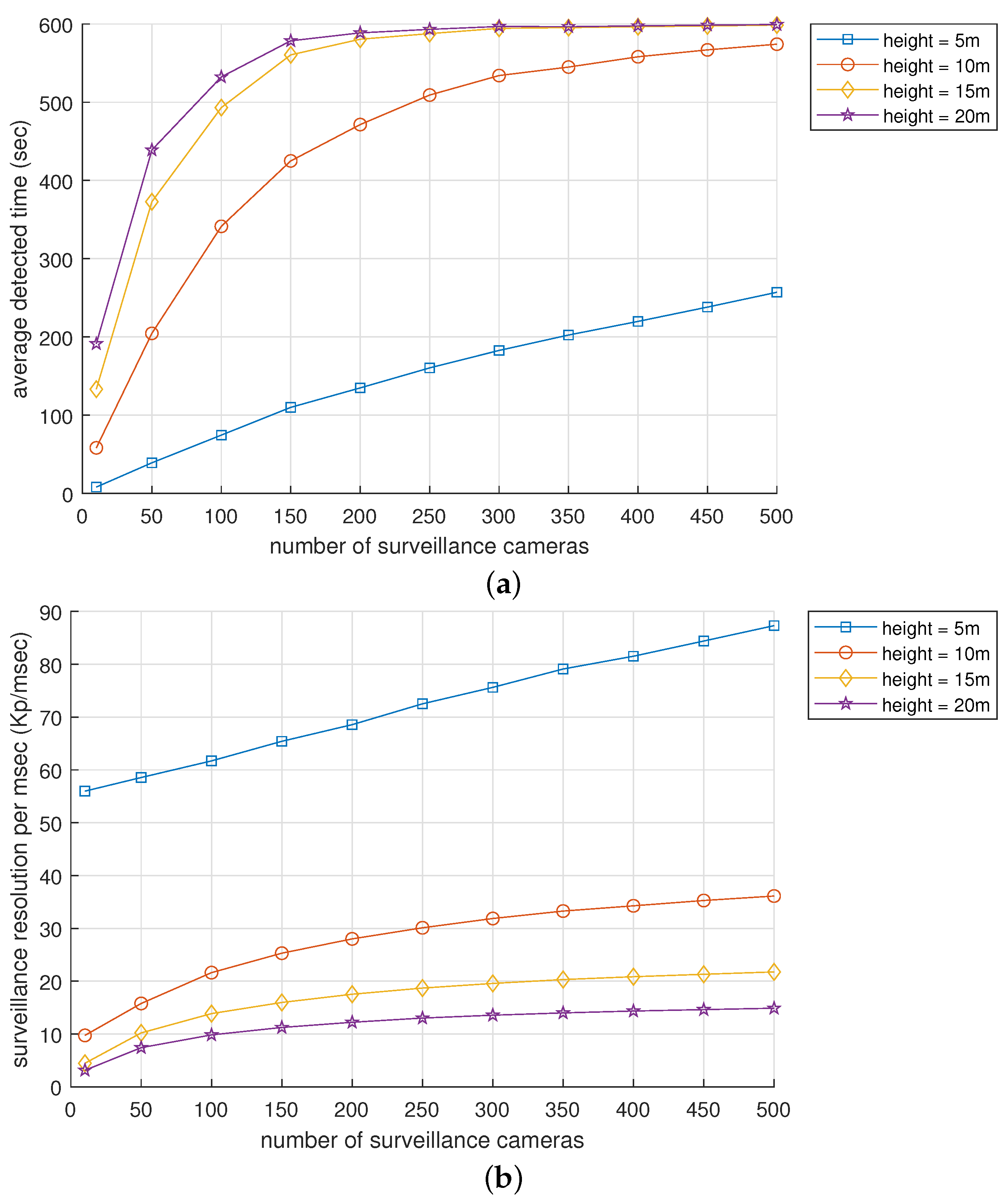
In this subsection, we will analyze the impact of surveillance camera installation height on the overall performance of the surveillance camera system. The simulation evaluated four different installation heights, which are 5 m, 10 m, 15 m, and 20 m. Figure 10a showcases the surveillance camera system’s performance, $T_{suc}$, as a function of the installation height. It is evident from Figure 10a that the higher the installation height of surveillance cameras, the longer the detection time. For instance, if the number of cameras is increased from 10 to 500, $T_{suc}$ at the height of 5 m increases from 8.2 s to 257.1 s. Similarly, at 10 m, $T_{suc}$ increases from 58.3 s to 574.2 s; at 15 m, $T_{suc}$ increases from 133.2 s to 598.6 s. Finally, at 20 m, $T_{suc}$ increases from 191.3 s to 599.2 s.

Comparing the heights of 5 m and 20 m, the difference in detection time ranges from approximately 2.2- to 23.5-fold higher, respectively. By adjusting the installation height of surveillance cameras, it is possible to achieve an acceptable performance concerning $T_{suc}$ with a lower camera density. For instance, if the camera height is set to 20 m, the pedestrian detection time is 96.4% of the total simulation time with only 150 cameras. This highlights the importance of the installation height of surveillance cameras in enhancing the performance of surveillance camera systems.

To summarize, the simulation results indicate that the installation height of surveillance cameras can significantly impact the $T_{suc}$ of the system. As the height of the surveillance cameras is increased, $T_{suc}$ also increases, leading to a longer detection time. Hence, adjusting the installation height of surveillance cameras to achieve an acceptable performance concerning $T_{suc}$ with a lower camera density is crucial.

The height of surveillance cameras plays a crucial role in the detection and identification of objects. Notably, the surveillance resolution of detected objects tends to decrease as the height of surveillance cameras increases. Therefore, it is essential to ensure that the surveillance resolution does not fall below a specific level to avoid any difficulty in detection or identification.

Figure 10b showcases the surveillance resolution value per ms based on the installation height of surveillance cameras and the number of cameras. Upon analyzing the data, it is evident that at a height of 5 m, the surveillance resolution per ms increases from 55.98 to 87.32 kilopixels/ms. Similarly, at 10 m, the surveillance resolution per ms rises from 9.74 to 36.13 kilopixels/ms, while at 15 m, it increases from 4.47 to 21.76 kilopixels/ms.

Moreover, at 20 m, the surveillance resolution per ms increases from 3.14 to 14.89 kilopixels/ms. The data reveal that increasing the installation height of surveillance cameras can lead to a decrease in the surveillance resolution per ms at 10 m, 15 m, and 20 m to 17.4%, 8.0%, and 5.6%, respectively, of the spatial resolution per ms at 5 m.

In conclusion, it is essential to maintain the optimal height of surveillance cameras to ensure effective detection and identification of objects. The data presented in Figure 10b can provide an insight into determining the appropriate installation height of surveillance cameras, keeping in mind the number of cameras and surveillance resolution per ms. It is crucial to note that the surveillance resolution per ms is a critical factor that should not be overlooked when installing surveillance cameras.

5. Conclusions and Future Works

In this paper, we introduced our designed system-level simulator by modeling the surveillance performance of cameras and devising several performance metrics to measure detection performance and quality. Since evaluating the performance of a system that operates many surveillance cameras in real time is challenging, our simulation approach could contribute to assessing surveillance system effectiveness in detecting and tracking criminal activities. In addition, the simulation results can provide comprehensive insights into surveillance system performance to optimize their design and improve public safety.

In future work, to make more practical use of our simulation methodology, we will focus on implementing the digital twin world, which imitates a city in the real world, based on open public data for a city and various other tools.