
Study of the Ecosystem Service Value Gradient at the Land–Water Interface Zone of the Xijiang River Mainstem
 ,
,
Abstract
:1. Introduction
Background
2. Materials and Methods
2.1. Data Sources
2.2. Research Methodology
2.2.1. Site Classification
2.2.2. Gradient Division at the Spatial Level
Gradient Division along the River
Upstream and Downstream Gradient Division
2.2.3. Method for ESV Evaluation in the Unit Area
2.2.4. ESV Driver Model Construction
3. Results
3.1. Overall Analysis
3.1.1. Characteristics of Land Use Types
3.1.2. The ESV in the Study Area
3.1.3. Value of the Four Major Ecosystem Services
3.2. The Lateral Gradient Analysis
3.2.1. Trends in the Value of Ecosystem Services at the Lateral ESV Gradient
3.2.2. Trends in Lateral Changes in the Value of the Four Major Ecosystem Services
3.3. Upstream and Downstream Gradient Analysis
Trends in the Value of Ecosystem Upstream and Downstream Gradient Levels
3.4. Analysis of ESV Drivers
3.4.1. General Characteristics of the Influence of Each Driving Factor on the ESV in the Study Area
3.4.2. Gradient Characteristics of the Effect of Each Driver on the ESV in the Study Area
4. Discussion
5. Conclusions
- (1)
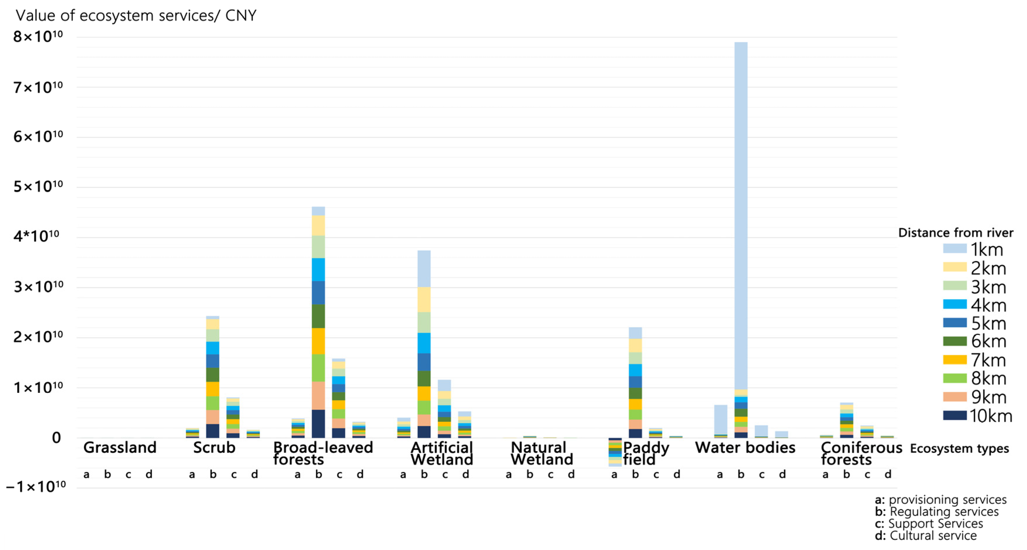
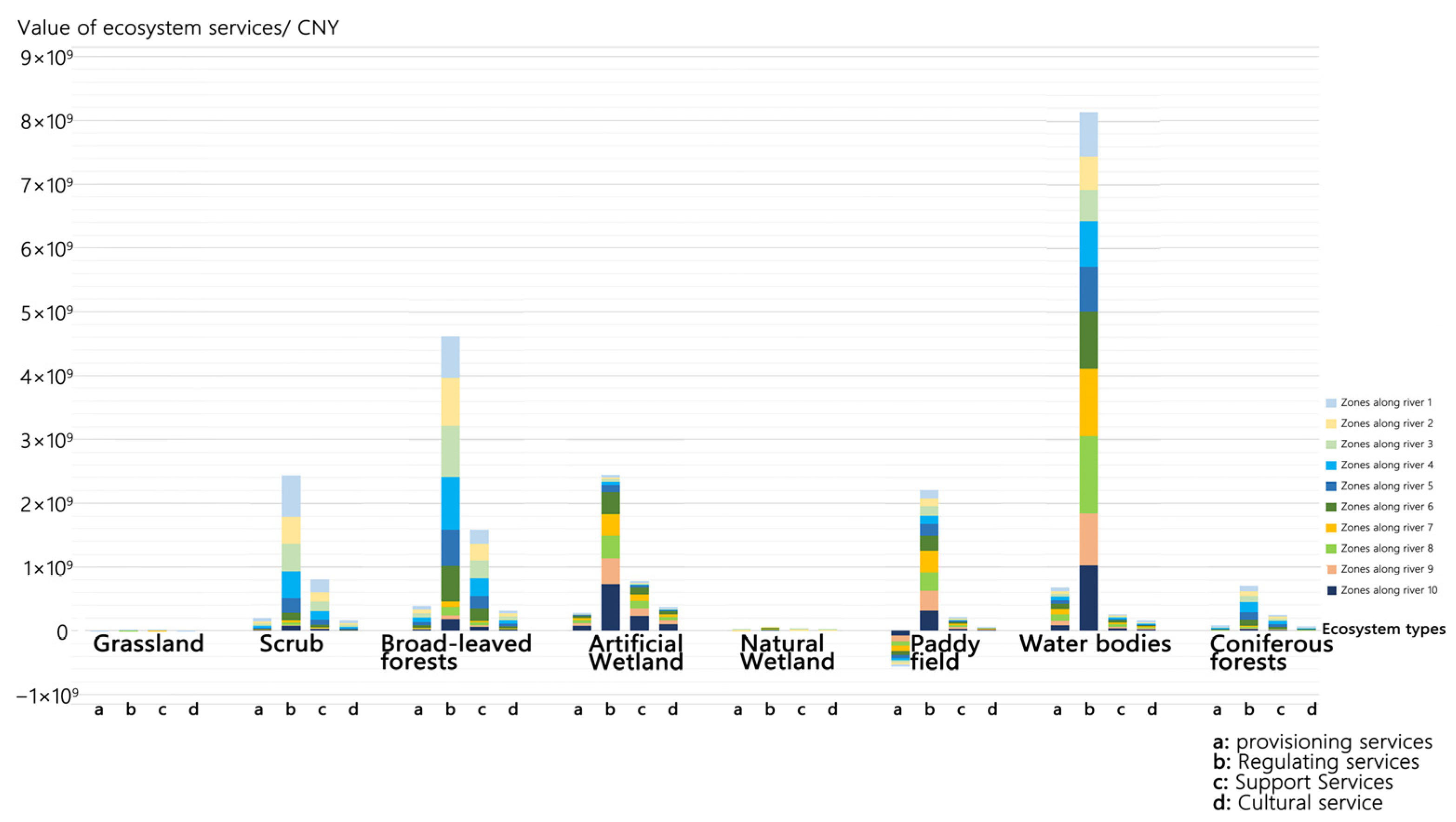
- The level of each type of ESV does not depend entirely on the size of the area but is determined by the ecosystem service functions it can provide and the level of ESV per unit area. Water bodies and wetland ecosystems provide the highest land-averaged ESVs of all ecosystem types and mainly provide provisioning and regulating services, further confirming the ecological importance of water bodies for hydrological regulation and climate regulation [46,47,48];
- (2)
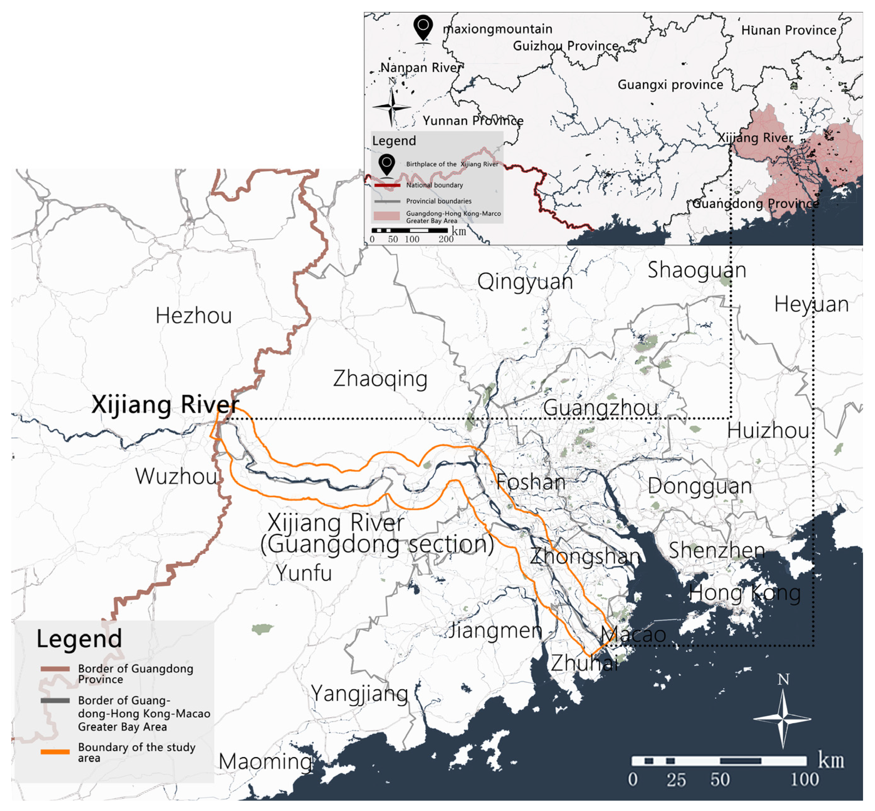
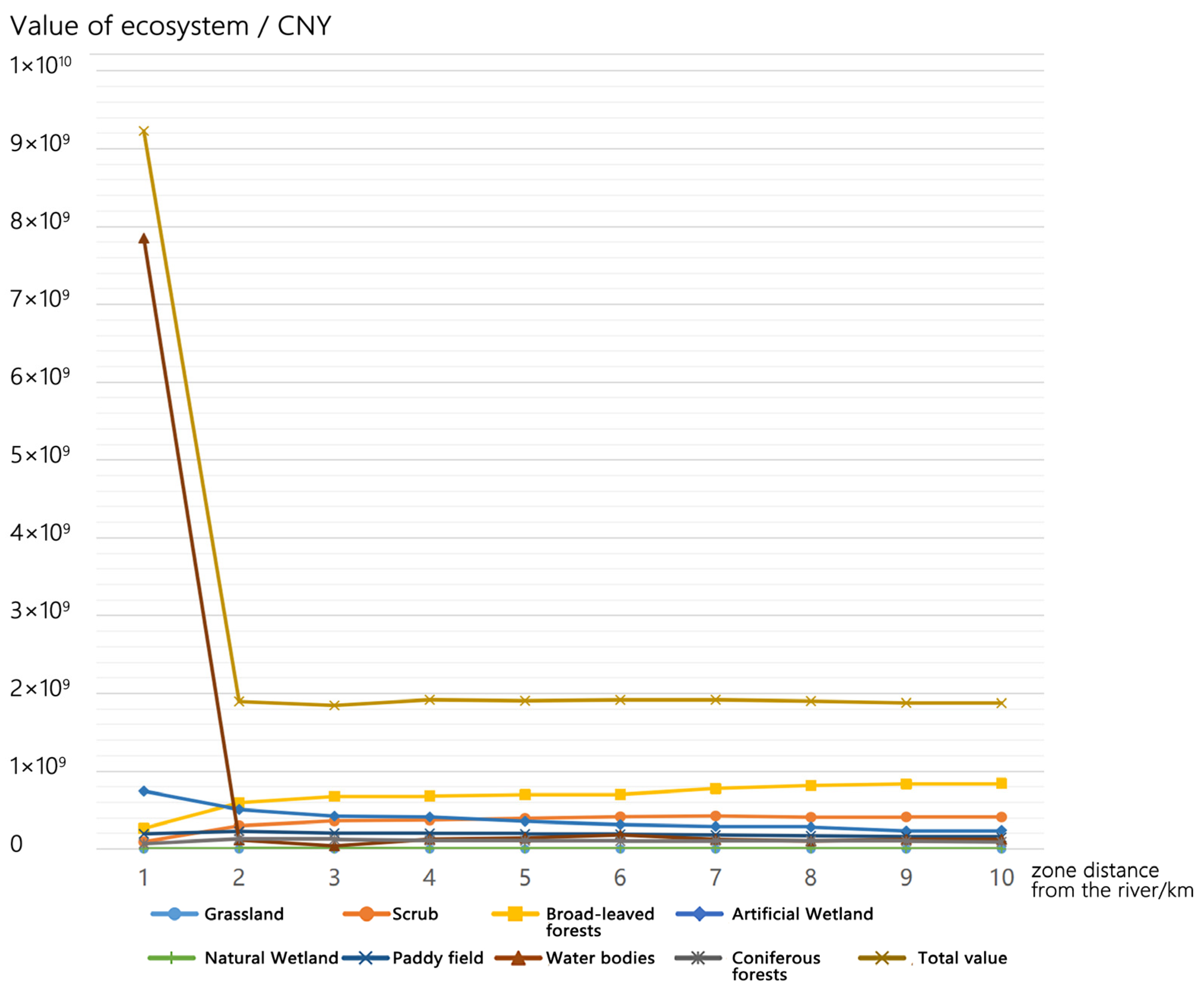
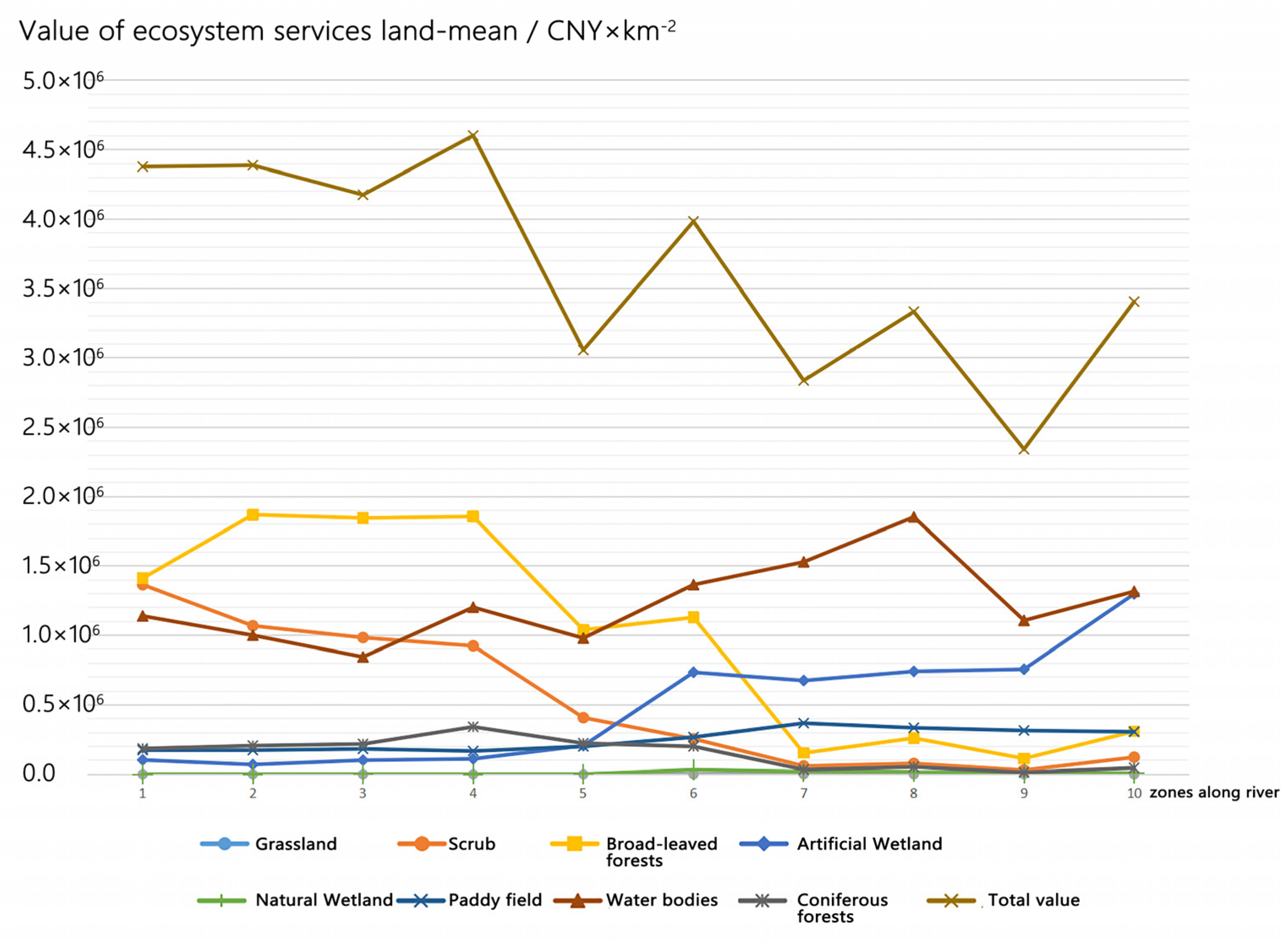
- The relationship between land use types on both sides of the Guangdong section of the Xijiang River Basin shows a trend from water ecosystems to terrestrial ecosystems, and the ESV decreases gradually with the increase in distance from the water. The trend in the ecosystem service value of the Xijiang River’s interface zone varying with the distance from the water bodies corroborates, to some extent, the superiority of the interface zone over the land in terms of ecological functions and values. It indicates that ecological protection measures within 1 km of the river should be increased at the water bodies scale, attention should be paid to the protection of forest land within 6–10 km, and artificial wetlands should be gradually replaced by natural wetlands to enhance the value of water bodies ecosystem services [49,50];
- (3)
- In relation to the Guangdong section of the Xijiang River Basin, the land-averaged ESV shows an overall undulating trend and decreases with decreasing distance from downstream areas. On the upstream and downstream gradient, because of the geographic environmental differences and urbanization development, the land use system at the upstream and downstream gradient in different regions changed subsequently, and the ecosystem structure gradually tended to develop into diversified forms, with broad-leaved forests as the main form. The land-averaged ESV showed a fluctuating and decreasing trend, and the landscape pattern showed an intensification of fragmentation, an increase in richness, and a trend of landscape diversification. Once again, this proves that different land use types and landscape spatial configurations will lead to landscape spatial heterogeneity, which, through landscape function conduction, will, to a certain extent, trigger spatial differences in ESVs, ultimately leading to spatial differences in ESVs, which shows that the higher the degree of landscape fragmentation and the higher the dispersion of landscape types, the lower the law of an ESV [51].
- (4)
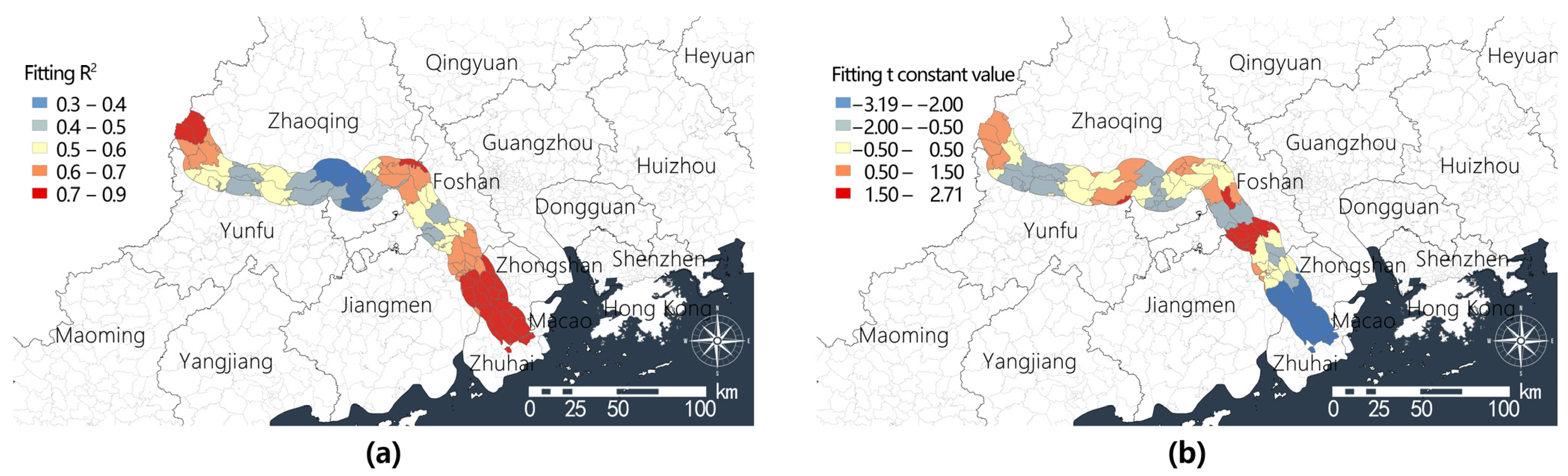
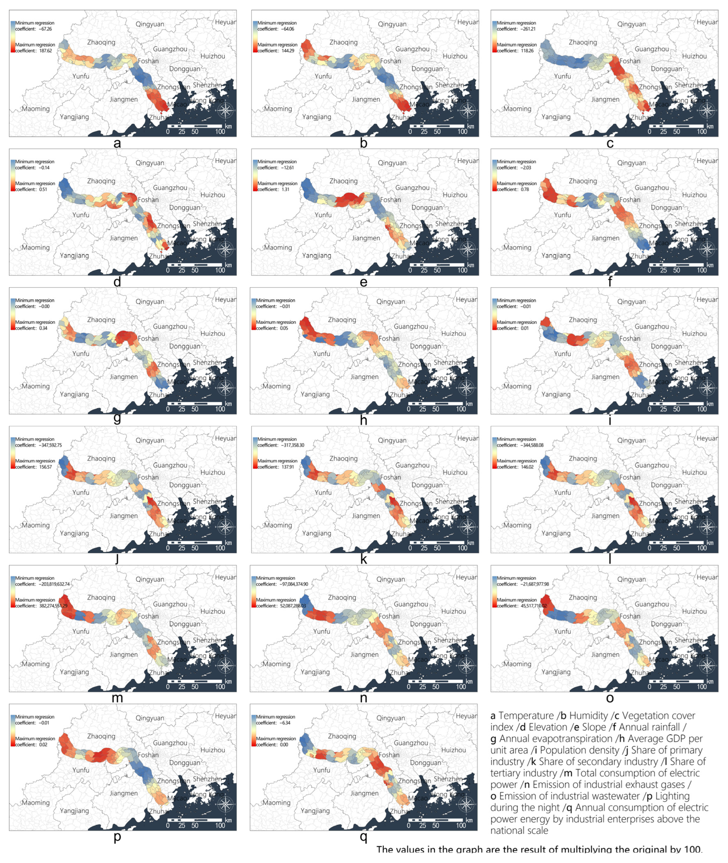
- By constructing a geographically weighted regression model to analyze the spatial differentiation characteristics and intrinsic causes of the impacts of natural systems and socio-economic factors on the value of land ecological services (ESV), it is known that the dominant drivers of ecosystem services in the waterway intersection zone of the Guangdong section of the Xijiang River mainstem are the total amount of electric power consumption, industrial exhaust gas emissions, and industrial wastewater emissions, which suggests that the socio-economic factors have a greater impact on the ESV in the economically developed areas. These factors are generated by human living and production activities, which indirectly affect the size of ESV by influencing factors such as temperature and gas. In the context of global warming, natural factors, such as temperature, humidity, and rainfall, in the basin and socio-economic factors, such as the share of industries in each county and city, affect the spatial distribution characteristics of ESV in the region, while topographic and geomorphological factors, such as slope and vegetation cover, and socio-economic factors, such as energy consumption, electricity, and the emission of industrial waste gases and wastewater, are the determinants of changes in the generation of the ESV. It shows that the enhancement of ESV in water bodies requires both the fulfillment of ecosystem services based on geographic characteristics and the adjustment of human approaches to land use and production and living to cope with a range of natural and anthropogenic issues, such as global economic recession, global warming, and sudden public health events [46,52,53,54,55].
Author Contributions
Funding
Institutional Review Board Statement
Informed Consent Statement
Data Availability Statement
Acknowledgments
Conflicts of Interest
References
- San-José, J.; Montes, R.; Mazorra, M.A.; Matute, N. Heterogeneity of the inland water-land palm ecotones (morichals) in the Orinoco lowlands, South America. Plant Ecol. 2010, 208, 259–269. [Google Scholar] [CrossRef]
- Malysheva, E.A.; Mazei, Y.A.; Yermokhin, M.V. Testate amoebae community pattern in different types of boundary structures at the water-land contact zone. Biol. Bull. 2013, 40, 823–831. [Google Scholar] [CrossRef]
- Lorens, B.; Gradziel, T.M.; Sugier, P. Changes in vegetation of restored water-land ecotone of Lake Bikcze (Polesie Lubelskie region, Eastern Poland) in the years 1993–1998. Pol. J. Ecol. 2003, 51, 175–182. [Google Scholar]
- Kenwick, R.A.; Shammin, M.R.; Sullivan, W.C. Preferences for riparian buffers. Landsc. Urban Plan. 2009, 91, 88–96. [Google Scholar] [CrossRef]
- Xiang, H.; Zhang, Y.; Richardson, J. Importance of Riparian Zone: Effects of Resource Availability at Land-water Interface. Riparian Ecol. Conserv. 2016, 3, 1–17. [Google Scholar] [CrossRef]
- National Academies of Sciences. Medicine, Progress Toward Restoring the Everglades: The Eighth Biennial Review–2020; The National Academies Press: Washington, DC, USA, 2021; p. 324. [Google Scholar]
- Seilheimer, T.S.; Mahoney, T.P.; Chow-Fraser, P. Comparative study of ecological indices for assessing human-induced disturbance in coastal wetlands of the Laurentian Great Lakes. Ecol. Indic. 2009, 9, 81–91. [Google Scholar] [CrossRef]
- Veldkornet, D.A. The Influence of Macroclimatic Drivers on the Macrophyte Phylogenetic Diversity in South African Estuaries. Diversity 2023, 15, 986. [Google Scholar] [CrossRef]
- Yahia Meddah, R.; Ghodbani, T.; Senouci, R.; Rabehi, W.; Duarte, L.; Teodoro, A.C. Estimation of the Coastal Vulnerability Index Using Multi-Criteria Decision Making: The Coastal Social–Ecological System of Rachgoun, Western Algeria. Sustainability 2023, 15, 12838. [Google Scholar] [CrossRef]
- Tan, J.; Chen, M.; Ao, C.; Zhao, G.; Lei, G.; Tang, Y.; Wang, B.; Li, A. Inducing flooding index for vegetation mapping in water-land ecotone with Sentinel-1 & Sentinel-2 images: A case study in Dongting Lake, China. Ecol. Indic. 2022, 144, 109448. [Google Scholar] [CrossRef]
- Zhang, T.; Gao, Q.; Xie, H.; Wu, Q.; Yu, Y.; Zhou, C.; Chen, Z.; Hu, H. Response of Water Yield to Future Climate Change Based on InVEST and CMIP6—A Case Study of the Chaohu Lake Basin. Sustainability 2022, 14, 14080. [Google Scholar] [CrossRef]
- Chen, Y.; Duo, L.; Zhao, D.; Zeng, Y.; Guo, X. The response of ecosystem vulnerability to climate change and human activities in the Poyang lake city group, China. Environ. Res. 2023, 233, 116473. [Google Scholar] [CrossRef] [PubMed]
- Wu, J.; Fan, X.; Li, K.; Wu, Y. Assessment of ecosystem service flow and optimization of spatial pattern of supply and demand matching in Pearl River Delta, China. Ecol. Indic. 2023, 153, 110452. [Google Scholar] [CrossRef]
- Finlayson, C.M. Millennium Ecosystem Assessment. In The Wetland Book: I: Structure and Function, Management and Methods; Finlayson, C.M., Everard, M., Irvine, K., McInnes, R.J., Middleton, B.A., van Dam, A.A., Davidson, N.C., Eds.; Springer: Dordrecht, The Netherlands, 2016; pp. 1–5. [Google Scholar]
- Enríquez-de-Salamanca, Á. Valuation of Ecosystem Services: A Source of Financing Mediterranean Loss-Making Forests. Small-Scale For. 2022, 22, 167–192. [Google Scholar] [CrossRef]
- Kreuter, U.P.; Harris, H.G.; Matlock, M.D.; Lacey, R.E. Change in ecosystem service values in the San Antonio area, Texas. Ecol. Econ. 2001, 39, 333–346. [Google Scholar] [CrossRef]
- Camacho-Valdez, V.; Ruiz-Luna, A.; Ghermandi, A.; Berlanga-Robles, C.A.; Nunes, P.A. Effects of land use changes on the ecosystem service values of coastal wetlands. Environ. Manag. 2014, 54, 852–864. [Google Scholar] [CrossRef] [PubMed]
- Wilson, M.A.; Carpenter, S.R. Economic Valuation of Freshwater Ecosystem Services in the United States: 1971–1997. Ecol. Appl. 1999, 9, 772–783. [Google Scholar]
- Bhagabati, N.K.; Ricketts, T.H.; Sulistyawan, T.B.S.; Conte, M.N.; Ennaanay, D.; Hadian, O.; Mckenzie, E.; Olwero, N.; Rosenthal, A.K.; Tallis, H.; et al. Ecosystem services reinforce Sumatran tiger conservation in land use plans. Biol. Conserv. 2014, 169, 147–156. [Google Scholar] [CrossRef]
- Rahman, W.A.H.S.W.A.; Misman, A.; Kasmani, S.; Omar, H.; Ariff, W.M.S.W.M.; Halim, W.A.Z.A. Evaluating ecosystem services in primary linkage 1 of the central forest spine in Peninsular Malaysia using InVEST: Preliminary results. In Proceedings of the 9th IGRSM International Conference and Exhibition on Geospatial & Remote Sensing (IGRSM 2018), Kuala Lumpur, Malaysia, 24–25 April 2018; Volume 169. [Google Scholar]
- Fontana, V.; Ebner, M.; Schirpke, U.; Ohndorf, M.; Pritsch, H.; Tappeiner, U.; Kurmayer, R.J.E.E. An integrative approach to evaluate ecosystem services of mountain lakes using multi-criteria decision analysis. Ecol. Econ. 2023, 204, 107678. [Google Scholar] [CrossRef]
- Bejagam, V.; Keesara, V.R.; Sridhar, V. Impacts of climate change on water provisional services in Tungabhadra basin using InVEST Model. River Res. Appl. 2022, 38, 94–106. [Google Scholar] [CrossRef]
- Dashtbozorgi, F.; Hedayatiaghmashhadi, A.; Dashtbozorgi, A.; Ruíz-Agudelo, C.A.; Fürst, C.; Cirella, G.T.; Naderi, M. Ecosystem services valuation using InVEST modeling: Case from southern Iranian mangrove forests. Reg. Stud. Mar. Sci. 2023, 60, 102813. [Google Scholar] [CrossRef]
- Caro, C.; Marques, J.C.; Cunha, P.P.; Teixeira, Z. Ecosystem services as a resilience descriptor in habitat risk assessment using the InVEST model. Ecol. Indic. 2020, 115, 106426. [Google Scholar] [CrossRef]
- Butsic, V.; Shapero, M.; Moanga, D.; Larson, S. Using InVEST to assess ecosystem services on conserved properties in Sonoma County, CA. Calif. Agric. 2017, 71, 81–89. [Google Scholar] [CrossRef]
- Xie, G.; Zhang, C.; Zhang, L.; Chen, W.; Li, S. Improvement of ecosystem service valorisation method based on value equivalent factor per unit area. J. Nat. Resour. 2015, 30, 1243–1254. (In Chinese) [Google Scholar]
- Pu, L.; Lu, C.; Yang, X.; Chen, X. Spatio-Temporal Variation of the Ecosystem Service Value in Qilian Mountain National Park (Gansu Area) Based on Land Use. Land 2023, 12, 201. [Google Scholar] [CrossRef]
- Zhao, X.A.-O.; Wang, J.; Su, J.; Sun, W. Ecosystem service value evaluation method in a complex ecological environment: A case study of Gansu Province, China. PLoS ONE 2021, 16, e0240272. [Google Scholar] [CrossRef]
- Taşyürek, M.; Celik, M. FastGTWR: A fast geographically and temporally weighted regression approach. J. Fac. Eng. Archit. Gazi Univ. 2021, 36, 715–726. [Google Scholar]
- Harris, P.; Fotheringham, A.S.; Crespo, R.; Charlton, M. The Use of Geographically Weighted Regression for Spatial Prediction: An Evaluation of Models Using Simulated Data Sets. Math. Geosci. 2010, 42, 657–680. [Google Scholar] [CrossRef]
- Czarnota, J.; Wheeler, D.C.; Gennings, C. Evaluating geographically weighted regression models for environmental chemical risk analysis. Cancer Inform. 2015, 14 (Suppl. S2), 117–127. [Google Scholar] [CrossRef]
- Li, L.; Phil, M. Research on Ecosystem Services Evaluation of the Modern Yellow River Delta Wetland Based on 3S Technology. Master’s Thesis, Shandong University of Science and Technology, Qingdao, China, 11 June 2011. [Google Scholar]
- Touseef, M.; Chen, L.; Masud, T.; Khan, A.; Yang, K.; Shahzad, A.; Wajid Ijaz, M.; Wang, Y. Assessment of the Future Climate Change Projections on Streamflow Hydrology and Water Availability over Upper Xijiang River Basin, China. Appl. Sci. 2020, 10, 3671. [Google Scholar] [CrossRef]
- Dars, G.H.; Strong, C.; Kochanski, A.K.; Ansari, K.; Ali, S.H. The Spatiotemporal Variability of Temperature and Precipitation over the Upper Indus Basin: An Evaluation of 15 Year WRF Simulations. Appl. Sci. 2020, 10, 1765. [Google Scholar] [CrossRef]
- Guangdong Water Resources Department. Xijiang River [EB/OL]. Available online: http://slt.gd.gov.cn/ysgk_new/lygk/xjly/index.html (accessed on 9 April 2023).
- Zhang, X.; Liu, L.; Chen, X.; Gao, Y.; Xie, S.; Mi, J. GLC_FCS30: Global land-cover product with fine classification system at 30 m using time-series Landsat imagery. Earth Syst. Sci. Data Discuss. 2020. [Google Scholar] [CrossRef]
- Costanza, R.; D’ARGE, R.; de Groot, R.; Farber, S.; Grasso, M.; Hannon, B.; Limburg, K.; Naeem, S.; O’Neill, R.V.; Paruelo, J.; et al. The value of the world’s ecosystem services and natural capital. Ecol. Econ. 1998, 25, 3–15. [Google Scholar] [CrossRef]
- Yu, X.; Gaodi, X.; Kai, A. Economic value of ecosystem services in Mangcuo Lake drainage basin. Chin. J. Appl. Ecol. 2003, 14, 676–680. (In Chinese) [Google Scholar]
- Department of Agriculture and Rural Affairs of Guangdong Province. Guangdong Plans to Upgrade One Million Mu of Ponds in the Pearl River Delta to Promote the Transformation and Upgrading of the Green Development of Aquaculture. Available online: http://dara.gd.gov.cn/mtbd5789/content/post_3518119.html (accessed on 14 September 2021).
- Yang, G.; Ouyang, Y.; Hou, X.; Zhou, T.; Ge, Y.; Lu, Y.; Wang, Y.; Chang, J. Homogenization of Urban Forests across the Subtropical Zones of China. Land 2023, 12, 1559. [Google Scholar] [CrossRef]
- Harrison, S.P.; Spasojevic, M.J.; Li, D. Climate and plant community diversity in space and time. Proc. Natl. Acad. Sci. USA 2020, 117, 4464–4470. [Google Scholar] [CrossRef] [PubMed]
- Zang, Z.; Zou, X.; Zuo, P.; Song, Q.; Wang, C.; Wang, J. Impact of landscape patterns on ecological vulnerability and ecosystem service values: An empirical analysis of Yancheng Nature Reserve in China. Ecol. Indic. 2017, 72, 142–152. [Google Scholar] [CrossRef]
- Muir, W.W. Regression Diagnostics: Identifying Influential Data and Sources of Collinearity; John Wiley & Sons: Hoboken, NJ, USA, 1980. [Google Scholar]
- Mach, M.E.; Martone, R.G.; Chan, K.M.A. Human impacts and ecosystem services: Insufficient research for trade-off evaluation. Ecosyst. Serv. 2015, 16, 112–120. [Google Scholar] [CrossRef]
- Yang, X.; Cai, H.; Zhang, X.; Zuo, T.; Chen, L. Spatial-temporal evolution of ecosystem service value and its driving factors in the Great Nanchang Metropolitan Area. Chin. J. Ecol. 2023, 14, 113. [Google Scholar]
- Millennium Ecosystem Assessment. Ecosystems and Human Well-Being: Synthesis; Island Press: Washington, DC, USA, 2005; Volume 7, p. 40. [Google Scholar]
- Mitsch, W.J.; Gosselink, J.G. The value of wetlands:mportance of scale and landscape setting. Ecol. Econ. 2000, 35, 25–33. [Google Scholar] [CrossRef]
- Uluocha, N.O.; Okeke, I.C. Implications of wetlands degradation for water resources management: Lessons from Nigeria. GeoJournal 2004, 61, 151–154. [Google Scholar] [CrossRef]
- Prach, K.; Hobbs, R.J. Spontaneous succession versus technical reclamation in the restoration of disturbed sites. Restor. Ecol. 2008, 16, 363–366. [Google Scholar] [CrossRef]
- Kroon, F. Wetland habitats: A practical guide to restoration and management/J1. Australas. J. Environ. Manag. 2011, 18, 265–266. [Google Scholar]
- Wei, L.; Luo, Y.; Wang, M.; Su, S.; Pi, J.; Li, G. Essential fragmentation metrics for agricultural policies: Linking landscape pattern, ecosystem service and land use management in urbanizing China. Agric. Syst. 2020, 182, 102833. [Google Scholar] [CrossRef]
- Zhu, M.; He, W.; Zhang, Q.; Xiong, Y.; Tan, S.; He, H. Spatial and temporal characteristics of soil conservation serice in the area of the upper and middle of the Yelow River, China. Heliyon 2019, 5, e2985. [Google Scholar] [CrossRef]
- Shoko, C.; Mutanga, O.; Dube, T. Reotely sensed C3 and C4 grass species abovearound biomass varablty in response to seasonal climate and topograchy. Afr. J. Ecol. 2019, 57, 477–489. [Google Scholar] [CrossRef]
- Muroz, J.D.; Steibel, J.; Snapp, S.; Kravchenko, A.N. Cover crop effect on corn growth and yield as infuenced by topography. Agric. Ecosyst. Environ. 2014, 189, 229–239. [Google Scholar]
- Fu, B.; Zhang, L. Land-use change and ecosystem services:Concepts, methods and progress. Prog. Geogr. 2014, 33, 441–446. [Google Scholar]


| Data Name | Data Description | Data Format/Accuracy | Data Source |
|---|---|---|---|
| Administrative boundary | Official government planning boundary | Shp | National Catalogue Service For Geographic Information “https://www.webmap.cn/main.do?method=index (accessed on 7 October 2022)” |
| Land use | Land use | Raster/30 m | Resource and Environment Science and Data Center, Chinese Academy of Sciences “www.resdc.cn (accessed on 7 October 2022)” |
| Temperature | Average annual surface temperature | Raster/1 km | |
| Humidity | Average annual surface humidity | Raster/1 km | |
| GDP per unit area | Average GDP per square kilometer | Raster/1 km | |
| Rainfall | Annual rainfall | Raster/1 km | |
| Evapotranspiration | Annual evapotranspiration | Raster/1 km | |
| Night light | Artificial night light | Raster/1 km | Geospatial data cloud platform “http://www.gscloud.cn/ (accessed on 24 January 2023)” |
| Elevation | Data of average elevation | Raster/30 m | |
| Vegetation cover index (NDVI) | Average annual NDVI | Raster/500 m | |
| Population density | Average population per square kilometer | Raster/1 km | Open Spatial Demographic Data and Research “https://hub.worldpop.org/ (accessed on 8 May 2023)” |
| Food production and food price data | Grain economic data of Guangdong Province | Excel | China Statistical Yearbook 2020, Guangdong Statistical Yearbook 2020, and China Statistical Information Network “http://www.tjcn.org/ (accessed on 8 May 2023)” |
| Industrial proportion | Proportion of primary, secondary, and tertiary industries | Excel | |
| Total electricity consumption | Total electricity consumption | Excel | |
| Industrial emissions | Industrial emissions | Excel | |
| Industrial wastewater discharge | Discharge of industrial wastewater | Excel | |
| Electricity and energy consumption of industrial enterprises above scale for the whole year | Discharge of industrial wastewater Annual power energy consumption of industrial enterprises above scale | Excel |
| Before Amendment | After Amendment | |||
|---|---|---|---|---|
| Ecosystem Services Classification | Classification | Wetlands | Wetlands | |
| Secondary Classification | Natural Wetlands | Natural Wetlands | Artificial Wetlands | |
| Supply service/CNY 104 | Food production | 0.51 | 0.51 | 0.3 |
| Raw material production | 0.5 | 0.5 | 0.3 | |
| Water supply | 2.59 | 2.59 | 1.7 | |
| Regulating services/CNY 104 | Gas regulation | 1.9 | 1.9 | 1.2 |
| Climate regulation | 3.6 | 3.6 | 2.4 | |
| Purification of the environment | 3.6 | 3.6 | 2.4 | |
| Hydrology | 24.23 | 24.23 | 15.8 | |
| Support services/CNY 104 | Soil conservation | 2.31 | 2.31 | 1.5 |
| Maintaining nutrient cycles | 0.18 | 0.18 | 0.1 | |
| Biodiversity | 7.87 | 7.87 | 5.1 | |
| Cultural service/CNY 104 | Aesthetics landscape | 4.73 | 4.73 | 3.1 |
| Type of Land Use | Area/km2 | The Proportion of the Area/% | Ecological Services Value/CNY 104 | The Proportion of ESV/% |
|---|---|---|---|---|
| Grassland | 0.24 | 0.00 | 61.68 | 0.00 |
| Scrub | 1056.47 | 15.60 | 360,747.12 | 13.72 |
| Built-up land | 1121.44 | 16.56 | 0.00 | 0.00 |
| Broad-leaved forest | 1342.16 | 19.82 | 691,059.56 | 26.28 |
| Artificial wetlands | 500.71 | 7.39 | 381,829.72 | 14.52 |
| Natural wetlands | 5.75 | 0.08 | 6705.38 | 0.25 |
| Paddy fields | 2156.18 | 31.84 | 188,176.53 | 7.16 |
| Water bodies | 317.66 | 4.69 | 894,546.93 | 34.02 |
| Coniferous forests | 271.22 | 4.01 | 106,669.80 | 4.06 |
| Total | 6771.83 | 100 | 2,629,796.72 | 100 |
| Type of Ecosystem | Provisioning Services | Regulating Services | Support Services | Cultural Services | ||||
|---|---|---|---|---|---|---|---|---|
| Value/CNY 104 | Proportion/% | Value/CNY 104 | Proportion/% | Value/CNY 104 | Proportion/% | Value/CNY 104 | Proportion/% | |
| Grassland ecosystems | 3.9 | 0.0039 | 39.8 | 0.002 | 14.9 | 0.0039 | 3 | 0.0028 |
| Scrub ecosystems | 19,909.8 | 19.9293 | 243,421.3 | 11.9546 | 81,061.4 | 20.9925 | 16,354.5 | 15.3531 |
| Broad-leaved forest ecosystems | 38,843.9 | 38.8818 | 461,910.8 | 22.6848 | 158,386.6 | 41.0174 | 31,918.2 | 29.9639 |
| Artificial wetland ecosystems | 25,837.1 | 25.8623 | 244,890.9 | 12.0268 | 75,264.6 | 19.4913 | 34,823.9 | 32.6917 |
| Natural wetland ecosystems | 464.0 | 0.4644 | 4296.2 | 0.211 | 1335.4 | 0.3458 | 609.7 | 0.5724 |
| Paddy field ecosystems | −57,081.8 | −57.1376 | 221,071.1 | 10.857 | 19,833.5 | 5.1363 | 4353.7 | 4.0871 |
| Water bodies ecosystems | 65,779.7 | 65.844 | 789,997.8 | 38.7973 | 25,299.9 | 6.5519 | 13,469.5 | 12.6448 |
| Coniferous forest ecosystems | 6145.8 | 6.1519 | 70,585.8 | 3.4665 | 24,948.4 | 6.4609 | 4989.7 | 4.6842 |
| Total | 99,902.4 | 100 | 2,036,213.7 | 100 | 386,144.7 | 100 | 106,522.2 | 100 |
| ESV of 1 km Distance/CNY 104 | ESV of 2 km Distance/CNY 104 | ESV of 3 km Distance/CNY 104 | ESV of 4 km Distance/CNY 104 | ESV of 5 km Distance/CNY 104 | ESV of 6 km Distance/CNY 104 | ESV of 7 km Distance/CNY 104 | ESV of 8 km Distance/CNY 104 | ESV of 9 km Distance/CNY 104 | ESV of 10 km Gradient/CNY 104 | |
|---|---|---|---|---|---|---|---|---|---|---|
| Grassland ecosystems | 4.7 | 4.4 | 6.0 | 6.1 | 7.2 | 7.0 | 9.4 | 5.1 | 6.3 | 5.5 |
| Scrub ecosystems | 9302.4 | 30,038.9 | 36,404.8 | 37,468.3 | 39,581.2 | 41,659.7 | 42,675.3 | 40,999.8 | 41,372.1 | 41,244.5 |
| Broad-leaved forest ecosystems | 26,667.4 | 59,654.1 | 67,788.0 | 68,334.9 | 69,998.7 | 70,345.7 | 78,040.7 | 81,837.1 | 83,906.7 | 84,486.3 |
| Artificial wetland ecosystems | 74,673.7 | 50,943.2 | 42,435.5 | 41,363.9 | 35,790.8 | 31,485.4 | 29,107.8 | 28,338.7 | 23,388.1 | 24,302.7 |
| Natural wetland ecosystems | 420.6 | 1064.0 | 874.0 | 645.1 | 664.1 | 742.0 | 712.0 | 570.7 | 471.8 | 541.0 |
| Paddy field ecosystems | 19,600.0 | 22,907.1 | 20,531.7 | 20,277.6 | 19,483.3 | 19,087.8 | 18,107.5 | 17,071.3 | 16,027.7 | 15,082.5 |
| Water bodies ecosystems | 785,207.2 | 11,877.8 | 4244.6 | 12,714.1 | 14,251.4 | 18,109.9 | 12,483.0 | 10,530.8 | 12,507.4 | 12,620.7 |
| Coniferous forest ecosystems | 7092.9 | 13,304.8 | 12,479.6 | 11,171.7 | 10,884.8 | 10,392.1 | 10,857.1 | 10,874.8 | 10,298.6 | 9313.6 |
| Total | 922,968.9 | 189,794.1 | 184,764.2 | 191,981.8 | 190,661.5 | 191,829.7 | 191,992.8 | 190,228.3 | 187,978.7 | 187,596.8 |
| Type of Land Use | Land Mean Ecosystem Service Value/CNY × km−2 | |||||||||
|---|---|---|---|---|---|---|---|---|---|---|
| Zones along River 1 | Zones along River 2 | Zones along River 3 | Zones along River 4 | Zones along River 5 | Zones along River 6 | Zones along River 7 | Zones along River 8 | Zones along River 9 | Zones along River 10 | |
| Grassland | 160.43 | 141.27 | 109.34 | 136.28 | 77.70 | 125.11 | 43.11 | 19.94 | 15.25 | 45.99 |
| Scrub | 1,365,599.32 | 1,069,295.79 | 984,299.26 | 925,022.31 | 407,431.00 | 254,341.65 | 58,517.80 | 76,776.86 | 29,088.37 | 122,059.18 |
| Construction | 0.00 | 0.00 | 0.00 | 0.00 | 0.00 | 0.00 | 0.00 | 0.00 | 0.00 | 0.00 |
| Broad-leaved forest | 1,412,518.28 | 1,869,851.60 | 1,845,724.86 | 1,856,288.68 | 1,039,748.70 | 1,129,807.40 | 152,100.26 | 259,970.98 | 112,668.96 | 308,159.35 |
| Artificial wetlands | 102,035.29 | 69,176.82 | 100,354.47 | 110,040.58 | 204,911.86 | 734,815.89 | 675,373.66 | 741,547.84 | 756,599.16 | 1,298,946.04 |
| Natural wetlands | 0.00 | 48.19 | 322.16 | 187.44 | 1591.64 | 32,075.69 | 19,596.50 | 15,711.19 | 8592.92 | 8355.62 |
| Paddy fields | 172,730.24 | 172,614.99 | 181,867.54 | 166,310.84 | 199,730.23 | 266,662.39 | 367,637.98 | 334,179.32 | 314,590.49 | 305,155.07 |
| Water bodies | 1,139,794.73 | 1,000,860.16 | 845,184.08 | 1,202,578.94 | 980,128.48 | 1,366,028.30 | 1,530,015.71 | 1,852,949.26 | 1,107,438.60 | 1,317,514.74 |
| Coniferous forests | 184,426.05 | 205,281.43 | 217,340.74 | 341,134.29 | 222,510.46 | 199,621.26 | 33,151.70 | 52,562.70 | 13,345.84 | 45,738.33 |
| Total | 4,377,264.34 | 4,387,270.27 | 4,175,202.44 | 4,601,699.36 | 3,056,130.08 | 3,983,477.70 | 2,836,436.72 | 3,333,718.08 | 2,342,339.59 | 3,405,974.33 |
| Driving Factor | Average Value | Standard Deviation | Maximum Value | Minimum Value | |
|---|---|---|---|---|---|
| Natural environmental factors | Temperature/°C | 23.14 | 0.77 | 24.10 | 18.90 |
| Humidity/%rh | 78.62 | 1.27 | 82.80 | 75.70 | |
| NDVI | 0.71 | 0.19 | 1.00 | 0.00 | |
| Elevation/m | 213.59 | 218.56 | 973.00 | 0.00 | |
| Slope/% | 12.34 | 6.01 | 66.45 | 0.00 | |
| Annual rainfall/mm | 1737.83 | 86.36 | 2004.25 | 1564.5 | |
| Annual evapotranspiration/kg·m−2 | 1082.19 | 145.78 | 1411.75 | 544.25 | |
| Socio-economic factors | GDP per unit area/CNY·km−2 | 8645.12 | 5954.76 | 153,465.00 | 501.00 |
| Population density/population·km−2 | 1115.68 | 1306.44 | 122,797.00 | 1.50 | |
| Proportion of primary industry/% | 14.41 | 11.49 | 37.9 | 0.03 | |
| Proportion of secondary industry/% | 43.61 | 11.88 | 75.60 | 22.70 | |
| Proportion of tertiary industry/% | 40.78 | 11.24 | 70.80 | 21.54 | |
| Total electricity consumption/108 KW·h | 271.16 | 193.74 | 710.30 | 78.56 | |
| Industrial emissions/104 t | 2481.89 | 753.73 | 3691.97 | 1057.7 | |
| Discharge of industrial wastewater/108·t | 6185.73 | 3354.09 | 11,455.08 | 1581.97 | |
| Night light/nWcm−2sr−1 | 24.86 | 18.41 | 59.52 | 0.01 | |
| Annual power energy consumption of industrial enterprises above designated size/104 KW·h | 303,192.90 | 329,690.49 | 1,079,429 | 29,301 |
| Zones along River 1 | Zones along River 2 | Zones along River 3 | Zones along River 4 | Zones along River 5 | Zones along River 6 | Zones along River 7 | Zones along River 8 | Zones along River 9 | Zones along River 10 | |
|---|---|---|---|---|---|---|---|---|---|---|
| Temperature | The topography of the region is predominantly mountainous, with high elevations, low average temperatures, low impacts from human activities, reduced human interference with ecology, and vegetation types dominated by broad-leaved evergreen forests, presenting positively driven characteristics. | The topography of the region is predominantly mountainous and hilly, with a decrease in elevation, an increase in average temperature, an increase in the impact of human activities, a high degree of development, a decrease in the percentage of broad-leaved forests and a decrease in the functioning of the woodland, which is characterized by a negative drive. | The region is positively driven by the impact of the construction of forest parks, which has increased the value of cultural services and support services. | The topography of the region is predominantly hilly with low elevations, and a high rate of urbanization in Foshan has resulted in a high level of ecological disturbance by humans and an increase in mean temperature, showing strong negative driving characteristics. | The region is close to the mouth of the sea, the terrain is dominated by plains, the atmosphere is affected by the cycle between land and water and ocean currents, the temperature is lowered, the climate is warmer and suitable for crop cultivation and growth, the proportion of paddy fields and artificial wetlands increases, and the value of provisioning services and the value of cultural services improves, presenting a stronger positively driven characteristic [39,40]. | |||||
| Humidity | The vegetation in the region is dominated by broad-leaved forests with high humidity, which has a more significant moderating effect and shows positive driving characteristics. | The vegetation in the region is dominated by coniferous forests, but the regional temperatures are higher than the optimal growth temperatures for coniferous forests, showing weak negative driving characteristics. | The area is positively driven by the construction of forest parks, which have increased humidity. | The region has a humid climate, increased human activities, and increased occupation of artificial wetlands, construction land, and paddy fields, crowding out the space of scrub and broad-leaved forest ecosystems, showing negative driving characteristics. | In regions with similar temperatures, water availability is a major determinant of the level of species diversity in different regions, and plant diversity is maximized in wetter climates, while wetter soils provide conditions for increased plant productivity [40,41]. Showing a clear positive driving effect. | |||||
| Vegetation cover index | Since the promotion of ESV by increasing NDVI is not a simple linear relationship, and there is a downward parabolic constraint on its promotion function, the promotion effect on both ESV and soil and water conservation services shows a characteristic of increasing and then decreasing with the increase in vegetation cover [42]. The region is mountainous with an average NDVI of 0.89, and when the NDVI exceeds 0.8, the plant cover continues to increase, and the promotion of ESV decreases. The various capacities of vegetation to contain water and soil retention reached the maximum growth threshold and then showed a decreasing trend. | The topography of the region is dominated by hills and plains, the population density increases, the vegetation cover decreases, similar to the threshold of the constraint line, and the regulating and supporting services of vegetation increase, showing obvious positive driving characteristics. | ||||||||
| Elevation | The terrain of the region is predominantly mountainous and sloping, prone to problems such as landslides and soil erosion, and unfavorable to human activities, with low value of provisioning services and cultural services, showing negative driving characteristics. | The terrain of the region is dominated by mountains and hills, with large slopes, increased impacts of human activities, a large degree of development, and a reduction in the function of forest land, but the construction of forest parks has a certain degree of ecological protection, showing weak negative drive characteristics. | The topography of the region is predominantly hilly with small slopes, and the impacts of human activities are further increased, with a consequent further reduction in woodland function, showing negative driving characteristics. | The topography of the region is dominated by plains with small slopes, high impacts of human activities, high degree of development, land use types dominated by paddy fields, artificial wetlands, and construction land, and crops are planted in large quantities, and the value of provisioning services and cultural services have been increased, which shows a weak negative driving characteristic. | ||||||
| Quantity of rainfall | The study area belongs to the subtropical monsoon climate zone, with abundant precipitation, which is conducive to the growth of vegetation and has a positive effect on the formation and evolution of the ecological environment, showing positive driving characteristics. | The topography of the region is dominated by hills, with reduced precipitation, and the area share of broad-leaved forests decreases, showing a weak negative correlation driving characteristics, but influenced by the construction of forest parks, part of the region shows weak positive driving characteristics. | The region’s gentle topography, frequent atmospheric circulation between land and sea, and increased rainfall are ecologically friendlier and exhibit positive driving characteristics. | The topography of the region is dominated by plains and is located at the mouth of the sea, which is highly influenced by ocean currents and ocean currents, and natural disasters such as flooding occur, causing damage to the ecosystem and presenting a weakly negatively driven character. | ||||||
| Share of primary industry | The primary industry in Fengkai County, to which the study area belongs, accounts for 37.9% of the total, with relatively backward production methods and high environmental burdens, showing negatively correlated driving characteristics. | The primary sector accounts for about 25% of the total but is limited by the mountainous terrain, with less human intervention and a small environmental burden, showing positively correlated driving characteristics. | The primary industry accounts for a relatively high proportion of the total, the intensity of human development is greater, and the impact on the environment is greater, showing strong negative correlation characteristics. | The primary industry accounts for a lower proportion of the population, the terrain is predominantly mountainous, and human activities are less destructive to the environment, showing a positive correlation with the driving characteristics. | The gradual flattening of the terrain and the increased development and utilization of agricultural land have led to the emergence of agricultural surface pollution, increasing the environmental burden and presenting a negatively correlated driving characteristic. | The share of the primary sector falls below 3%, which reduces the environmental impact and characterizes the positive correlation drive. | The proportion of primary industry has rebounded to about 8%, and with the construction of agriculture as one of the advantages of economic development, man-made interference has increased, increasing the burden on the environment and showing a strong negative correlation characteristics. | The primary sector’s share fell to below 3%, reducing the environmental burden and showing positively correlated driving characteristics. | ||
| Share of secondary industry | The industries in Fenkai County are dominated by traditional manufacturing industries such as non-ferrous metal smelting and rolling processing industries, which have obvious negative impacts on the environment and, therefore, show strong negative correlation driving characteristics. | The region’s secondary sector accounts for less than 30% of the total, reducing the pressure on the ecosystem and showing positive correlation driving characteristics. | The region’s secondary industry has increased its share to between 35 and 50% and is dominated by traditional industries, increasing environmental pressure and showing strong negative correlation-driving characteristics. | Industry accounts for a high proportion of the total but is characterized by a weak negative correlation drive as it follows the concept of green and circular development to mitigate environmental pressure. | The secondary industry has developed strongly, accounting for about 40–70% of the total, forming clusters of automobile parts, hardware, chemicals, new building materials, etc. The environmental pressure is high, showing a strong negative correlation driving characteristic. | Sanshui District secondary industry accounted for about 70% industry to be transformed and upgraded, showing a strong negative correlation characteristics; Nanhai and Gaoming Districts emerging industries are developing well, easing the pressure on the environment, showing a positive correlation driving characteristics. | The region’s secondary industry is in a period of transformation and upgrading, and its effect on environmental pressure mitigation has not yet been prominent, showing a negative correlation and driving characteristics. | The secondary industry in the region accounts for about 50–70%, but the economic benefits brought by development are promptly fed back into the investment in ecological environmental protection and management, instead promoting the improvement of the local ecological environment, showing a positive correlation driving characteristics. | ||
| Share of tertiary sector | Fengkai County’s tertiary industry accounts for 29.7% of the total, with a backward industrial structure and a large environmental burden, showing a strong negative correlation driving characteristics. | The tertiary sector, which accounts for about 40–50% of the total, is less damaging to the ecosystem and shows a strong positive correlation driving characteristic. | Bordering the fourth level of the river section, which exhibits negative correlation driving characteristics, contributes less to ESV because its terrain is predominantly mountainous and less developed for cultural services. | The tertiary industry in the region accounts for about 35.1%, and its share is increasing year by year. The industrial structure is in the process of transformation and upgrading, which is conducive to reducing the burden on the environment, showing a weak negative correlation driving characteristics. | Dinghu District in Zhaoqing City is affected by the construction of the park. Tertiary industry accounted for about 50%, but the tertiary industry in Gaoyao District accounted for only 28.6%, and the industrial structure is more backward, so the overall negative correlation drives the characteristics. | Bordering with the eighth level of the river section shows positive correlation driving characteristics, although the proportion of tertiary industry in Gaoming District is only 21.54%, but the emerging entrepreneurship is well constructed, and the tertiary industry is in an accelerated stage of establishment; meanwhile, the tertiary industry in Nanhai District accounts for 43.55% of the total, which is less burdensome to the environment. | The proportion of tertiary industry in this area is about 60–70%. Although the proportion is high, the development of tertiary industry is more inclined to cultural and entertainment services, construction services, and other service industries that encroach on the ecological land. | The tertiary industry in the region accounts for about 45–70% of the total, and the overall industrial structure is good and less damaging to the ecosystem, showing a positive correlation driving characteristics. | ||
| Total electricity consumption | The region is characterized by less total electrical consumption, less economic activity, and a lower burden of environmental pressures, showing a strong positive correlation drive. | The region borders the second level of the river section, where total electrical consumption increases, and the population concentrates there, causing more environmental disturbances and showing negatively correlated driving characteristics while bordering the fourth level of the river section, where total electrical consumption decreases and economic activity decreases, reducing environmental pressures and showing positively correlated driving characteristics. | Industrial development in the region has a higher electrical demand and more economic activity, which, to some extent, increases the environmental pressure, showing a negative correlation with driving characteristics. | The total amount of electrical consumption in the region has increased, and it is a plain area that is suitable for human activities and increased economic activities. In addition, the region has good landscape resources and a high degree of development of ecosystem cultural services, such as the construction of the National Forest Park in Dinghu District, thus showing an overall positive correlation driving characteristics. | The total electrical consumption in the region is the highest in the upstream and downstream gradient, indicating that the region has a higher demand for electrical in all sectors, more frequent economic activities, and, therefore, a heavy burden on the environment, showing a negative correlation driving characteristics. | The region has a high total electrical consumption but a good industrial structure and a more balanced demand, which facilitates the mitigation of environmental pressures and shows a positive correlation driving characteristics. | The region is characterized by a negative correlation driven by an increase in total electrical consumption, an increase in economic activity, and an increase in anthropogenic interventions. | |||
| Industrial emissions | The proportion of industry in the area is small; the traditional regional industries rely on energy and resources to a high degree, and the exhaust emissions are relatively small but are subject to the level of science and technology and management; there is the behavior of direct and stealthy exhaust emissions. It shows weak negative correlation driving characteristics. | The proportion of industry in this region has increased, mainly in the traditional manufacturing industry. Negative factors such as industrial sulfur dioxide and soot emissions in urban areas have brought huge purification pressure to the ecological environment, showing a negative correlation with driving characteristics. | In this region, Foshan City has a deep industrial development foundation and a good economic development trend. At the same time, it attaches great importance to industrial pollution remediation work and has achieved great results in waste gas treatment, reducing environmental pressure. However, industrial emissions still have an ecological impact, showing a negative correlation drive characteristic. | In parts of Jiangmen City and Zhongshan City in the region, industry accounts for a relatively high proportion of industrial emissions, such as sulfur dioxide and other industrial emissions, which aggravates the burden on the environment, showing a negative correlation driving characteristics. | The proportion of industry in this region is reduced, the pollution source is reduced, and the environmental burden is reduced. However, industrial emissions still have an early ecological impact, showing negative correlation driving characteristics. | |||||
| Industrial wastewater discharge | The proportion of industry in this area is small, and the industry is mainly based on the processing of building materials with low wastewater discharge. However, constrained by the level of science and technology and management level, the degree of wastewater treatment is low, and there is direct and smuggled discharge into the river. Weak support regulating services jeopardizes the environment, presenting weak negative driving characteristics. | The industrial structure of Deqing County of Zhaoqing city and Yun’an District of Yunfu City is upgraded. Wastewater discharges increase, showing negative driving characteristics. | In this region, Duanzhou District and Gaoyao District of Zhaoqing City are dominated by the high-tech and manufacturing industries. In Dinghu District, Sihui city, the traditional manufacturing industry accounts for a relatively large portion, all showing negative driving characteristics. | Foshan City pollution remediation work is good, and through Forest City construction, the environmental pressure is small, mostly showing weak negative driving characteristics. Among them, Sanshui and Shunde districts are intensive in secondary industries, and industrial wastewater has a certain impact on the environment, showing patchy negative driving characteristics. | In this area, the industrial proportion of Xinhui District in Jiangmen City is large, and the industrial wastewater has a great impact on the environment. In Zhongshan city, the proportion of traditional industries near inland areas is large, while the proportion of industries near Zhuhai and Macao is gradually decreasing, the proportion of service industries is increasing, and the discharge of industrial wastewater is reduced. In addition, the city is close to the estuary, which is influenced by ocean currents and accelerates the water cycle, showing positive and negative driving characteristics of regionalization. | |||||
Disclaimer/Publisher’s Note: The statements, opinions and data contained in all publications are solely those of the individual author(s) and contributor(s) and not of MDPI and/or the editor(s). MDPI and/or the editor(s) disclaim responsibility for any injury to people or property resulting from any ideas, methods, instructions or products referred to in the content. |
© 2023 by the authors. Licensee MDPI, Basel, Switzerland. This article is an open access article distributed under the terms and conditions of the Creative Commons Attribution (CC BY) license (https://creativecommons.org/licenses/by/4.0/).
Share and Cite
Huang, Y.; Deng, J.; Xiao, M.; Huang, Y.; Li, H.; Xiao, Y.; Huang, Y. Study of the Ecosystem Service Value Gradient at the Land–Water Interface Zone of the Xijiang River Mainstem. Appl. Sci. 2023, 13, 10485. https://doi.org/10.3390/app131810485
Huang Y, Deng J, Xiao M, Huang Y, Li H, Xiao Y, Huang Y. Study of the Ecosystem Service Value Gradient at the Land–Water Interface Zone of the Xijiang River Mainstem. Applied Sciences. 2023; 13(18):10485. https://doi.org/10.3390/app131810485
Chicago/Turabian StyleHuang, Yang, Junling Deng, Min Xiao, Yujie Huang, Hui Li, Yinyin Xiao, and Yiting Huang. 2023. "Study of the Ecosystem Service Value Gradient at the Land–Water Interface Zone of the Xijiang River Mainstem" Applied Sciences 13, no. 18: 10485. https://doi.org/10.3390/app131810485