Adaptive Impedance Control for Force Tracking in Manipulators Based on Fractional-Order PID

Abstract

Force tracking control in robot arms has been widely used in many industrial applications, particularly in tasks involving end effectors and environmental contact, such as grinding, polishing, and other similar operations. However, these environments are not always precisely known. In order to address the force tracking control problem in unknown environments, this paper proposes a fractional-order PID adaptive impedance control strategy based on traditional impedance control. The unknown environmental information is estimated online using the adaptive impedance control algorithm, and the estimated parameters are used to generate reference trajectories to reduce force tracking errors. Fractional-order PID control is then introduced into the system to improve the control performance of the system model, and the theoretical proof of strategy stability is conducted. Finally, a comparison of four strategies was conducted through simulations: traditional impedance control, adaptive hybrid impedance control, adaptive variable impedance control, and the fractional-order PID impedance control proposed in this paper. The simulation results demonstrate that the strategy proposed in this paper exhibits robustness, virtually eliminates overshoot, and enhances response speed. In contrast, both adaptive hybrid impedance control and adaptive variable impedance control exhibit approximately 30% to 45% overshoot during interactions with the environment. Furthermore, in terms of force tracking error, the proposed strategy in this paper outperforms the above two strategies by approximately 29% to 60%, achieving excellent force tracking control performance.

1. Introduction

As we look to the future, it seems likely that robots will assume a range of new roles in people’s daily lives [1]. They may replace human labor in some industries, provide valuable services, or even offer specialized training to individuals [2]. Some people, when compared to communicating with humans in daily life, even prefer to use robots as communication partners in many roles and situations [3]. These developments promise to revolutionize the way we live and work, giving rise to new possibilities and transforming our daily routines in unexpected ways [4]. In recent years, robots have become an increasingly common sight in a variety of human environments, including nursing homes, hospitals, shopping malls, and the education industry [5,6]. In the field of robotics, there has long been a focus on designing and controlling robots that can interact with their environment, particularly in cases where the objects of interaction are human [7].

As robots become increasingly integrated into open working environments, it is inevitable that robots will come into contact and interact with humans [8], and ensuring safe interactions between these machines and humans is becoming a key area of focus in robotics research. When humans provide motion correction, fine-tuning control, and situational guidance to working robots, the proximity required for these interactions can pose a significant risk of injury. This challenge has driven the development of new approaches to robot control, with an emphasis on creating security rules that enable safe and controlled physical interactions between robots, humans, and the environment [9,10]. Therefore, to guarantee the safety of the surrounding environment and humans around robots, it is necessary to study the interaction mechanisms that enable robots to adapt to the surrounding environment [11,12]. In addition, there is a need to balance the compliance and accuracy of the robot.

Impedance control was first proposed by Hogan [13], and later Kazeroni developed and implemented an automated impedance control method for the precise deburring of industrial robots to replace the time-consuming and expensive manual deburring approach [14]. However, impedance control still faces many challenges: the nonlinear and time-varying characteristics of the robot’s own dynamics and kinematics make it insufficient to rely solely on impedance control to solve practical problems [15]. Therefore, in practical applications, impedance control is often combined with other control methods, such as adaptive control.

In Oladayo’s study [16], an adaptive force tracking impedance controller was developed, and the controller’s parameters were adjusted using a genetic algorithm (GA) under force-torque constraints. The controller adjusts the contact force by adapting the target stiffness in response to changes in the stiffness of the contact environment, with the aim of achieving adaptive control. In a study by Wei et al. [17], a force-based impedance control system was designed, and three self-calibrating functions for impedance parameters were constructed to improve the design of the impedance control system to achieve adaptive control. Chen et al. [18] optimized the PD control parameters by using particle swarm optimization and adaptive iterative algorithms based on the robot’s machining state. K. Wakita et al. [19] optimized a robot’s position control and reference trajectory by estimating human movement direction and using a Kalman filter, and they also achieved adaptive control for robots.

However, some adaptive impedance control methods, while showing promising performance compared to traditional impedance control, still have many issues. Zhou H et al. [20] proposed an adaptive control-based hybrid impedance control strategy for achieving compliant force control in industrial robots. Thunyajarern et al. [21] presented an adaptive force controller for six degrees of freedom robots and addressed the environmental identification problem by using particle swarm optimization. However, the optimization algorithm was performed offline and did not yield a satisfactory adaptation to the environment. Zhou Y et al. [22] proposed a variable impedance control algorithm that achieved superior force tracking control when compared to traditional impedance control. However, the end effector exhibited significant overshoot when in contact with the environment, potentially leading to equipment damage. Cao et al. [23] combined PID controllers with impedance control to enhance control performance during contact. However, traditional PID controllers have limited degrees of freedom and are prone to integral saturation. Li et al. [24] incorporated PID control into the design of a model reference adaptive impedance controller to improve impedance relationships. Nevertheless, significant overshoot still exists during the contact process, and a stability analysis of a system after introducing PID has not been provided. Zhao et al. [25] proposed an improved fractional-order PID impedance control method based on traditional impedance control, achieving good force tracking control results. However, their proposed method lacks theoretical derivation of its validity and stability.

In order to address the issues and limitations observed in the aforementioned control algorithms, such as overshooting during robotic contact with the environment, offline algorithm optimization, and the lack of corresponding stability theory derivation, this paper proposes a fractional-order PID adaptive impedance control strategy and provides theoretical stability and validity derivations. This strategy allows for the real-time dynamic estimation of environmental information in uncertain and changing environments. It updates the reference trajectory in real-time based on estimated parameters to achieve adaptive control. Additionally, the flexibility of fractional-order PID further enhances force tracking control performance in complex environments, minimizing overshoot and maintaining stable force tracking. This ensures equipment safety and smooth task execution in applications with stringent machining precision requirements within complex environments.

The main contributions of this paper are as follows: a fractional-order PID adaptive impedance control strategy was proposed to enhance the performance of robotic interactions with the environment and the subsequent force tracking; a mathematical derivation of the rationality and stability of the proposed strategy; and the validation of its superiority through comparative simulations.

The remaining parts of the paper are organized as follows. Section 2 describes the impedance control system studied in this paper. Section 3 analyzes the stability of the impedance model and presents the design of the adaptive control with an online estimation of environmental parameters. Section 4 proposes the design of the fractional-order PID impedance controller and provides the theoretical proof of stability. Section 5 sets up simulations to validate the proposed strategy. Finally, Section 6 provides the conclusion of the paper.

2. System Description

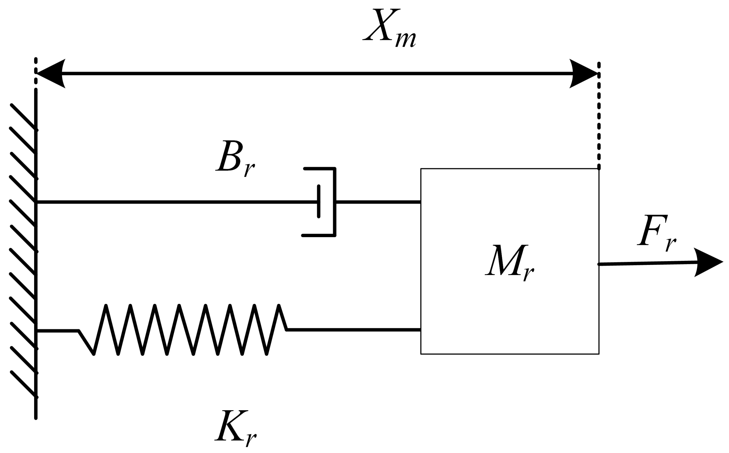
2.1. Force Interaction Model

Generally, the process of a robot coming into contact with an unknown environment can be described as transitioning from free-space motion to contact and then to gradually stabilizing the contact forces. The contact process is shown in Figure 1.

During the contact process, the dynamic characteristics of the robot and the behavior of the contact force vary at different stages. Figure 2 shows the variation of contact force during the contact process.

As shown in Figure 2, the contact process of the robot can be divided into three stages:

• Stage I: linear motion in free space when approaching the environment.
• Stage II: a nonlinear region with significant overshoot and intense collision when contact occurs.
• Stage III: an approximately linear region where the contact force gradually stabilizes after contact.

This paper focuses on Stage II and Stage III after contact, as Stage I is a basic ability that the robot should possess.

2.2. Impedance Control Model

The core idea of impedance control is to transform almost all physical systems into a “mass-spring-damper” system, as shown in Figure 3, and the force situation of this system can be expressed as

$$F=M_r\ddot{E}+B_r\dot{E}+K_{r}E$$

(1)

In the equation, $E=X_d-X_m$, where $X_d$ is the desired position, and $X_m$ is the actual position. $M_r$ is the desired inertial matrix, $B_r$ is the desired damping matrix, and $K_r$ is the desired stiffness matrix.

This paper employs position-based impedance control (sometimes referred to as admittance control) [26] to manipulate industrial robots. This control structure consists of an internal position control loop and an external force control loop, which equates the controller to an admittance system: input force; output position and equates the robot to an impedance system: input position; output force. Overall, it maps from force to position. The schematic diagram is shown in Figure 4.

Where $X_r$ is the reference trajectory corresponding to the expected force, $X_d$ denotes the trajectory information sent by the impedance model to the robot, and X represents the trajectory information of the end effector of the robot’s actual movement. In the position control mode, $X_d$ is usually equal to X, and the trajectory error caused by contact force can be expressed as $E=X-X_r=X_d-X_r$. $F_r$ is the desired tracking force, $F_e$ is the actual contact force, and the error between the two is $\Delta F=F_e-F_r$.

Usually, the error force $\Delta F$ is represented as a linear second-order system, as shown in Equation (1), which can be obtained by substituting F and E into it.

$$M_r({\ddot{X}}_r-{\ddot{X}}_d)+B_r({\dot{X}}_r-{\dot{X}}_d)+K_r(X_r-X_d)=F_e-F_r$$

(2)

where $M_r$ is the desired inertia matrix, $B_r$ is the desired damping matrix, and $K_r$ is the desired stiffness matrix. The impedance model is a second-order transfer function:

$$H\left(s\right)=\frac{E\left(s\right)}{\Delta F\left(s\right)}=\frac{1}{M_r{s}^2+B_{r}s+K_r}$$

(3)

where the force error $\Delta F=F_e-F_r$ and the position error $E=X_r-X_d$, from which the trajectory information sent to the robot can be obtained as $X_d=X_r+E$.

3. Adaptive Control System

3.1. Stability Analysis of Impedance Control Models

Usually, the model parameters, $M_r$, $B_r$, and $K_r$, of the impedance controller and the environmental dynamics parameters, $K_e$, are positive definite diagonal matrices, with the forces in each direction decoupled. Therefore, for the convenience of subsequent research analysis in this paper, the applied force is decomposed and studied. It is assumed that the contact force only acts in one direction, which is the direction of the force. Lowercase letters x, $x_r$, $x_d$, $m_r$, $b_r$, $k_r$, $f_r$, $f_e$, $x_e$, $k_e$, and $b_e$ are used to represent variables and coefficients in a single direction, respectively, instead of the uppercase letters X, $X_r$, $X_d$, $M_r$, $B_r$, $K_r$, $F_r$, $F_e$, $X_e$, $K_e$, and $B_e$. Thus, the impedance relationship in Equation (2) can be expressed in a single direction:

$$m\left({\ddot{x}}_r-{\ddot{x}}_d\right)+b\left({\dot{x}}_r-{\dot{x}}_d\right)+k\left(x_r-x_d\right)=f_e-f_r=-\Delta f$$

(4)

We assume the environmental dynamics model to be as is shown in Equation (5), where $x_e$, $k_e$, and $b_e$ represent the environmental position, environmental stiffness, and environmental damping, respectively.

$$f_e=b_e(\dot{x}-{\dot{x}}_e)+k_e(x-x_e)$$

(5)

Additionally, when the robot makes contact with the environment, its acceleration and movement speed are very small, and the contact force between the robot and the environment can be simplified to

$$f_e=k_e(x-x_e),x>x_e$$

(6)

Taking the Laplace transform of Equation (4) yields

$$(m_r{s}^2+b_{r}s+k_r)\left(x_d\left(s\right)-x_r\left(s\right)\right)=\left(f_r\left(s\right)-f_e\left(s\right)\right)=\Delta f\left(s\right)$$

(7)

By transforming and further simplifying Equation (7), we obtain

$$\begin{array}{c}\left(x_d\left(s\right)-x_r\left(s\right)\right)=\frac{1}{(m_r{s}^2+b_{r}s+k_r)}\left(f_r\left(s\right)-f_e\left(s\right)\right)\\ e\left(s\right)=H\left(s\right)\Delta f\left(s\right)\end{array}$$

(8)

where $H\left(s\right)=1/(m_r{s}^2+b_{r}s+k_r)$ is the transfer function, as shown in Equation (3). It represents the desired impedance model of the robotic arm, which converts the force error during the contact process into a correction for the reference trajectory.

Taking the Laplace transform of the environmental dynamics model shown in Equation (6) yields

$$f_e\left(s\right)=k_e\left(x\left(s\right)-x_e\left(s\right)\right),x>x_e$$

(9)

As mentioned in Section 2.2, it is generally assumed that there is no tracking error in the position control mode of the robot, that is, $x=x_d$. By incorporating the desired force into Equation (9), we obtain

$$\Delta f\left(s\right)=f_r\left(s\right)-k_e\left(x_d\left(s\right)-x_e\left(s\right)\right)$$

(10)

Substituting Equation (8) into Equation (10) yields

$$\Delta f\left(s\right)=f_r\left(s\right)-k_e\left(x_r\left(s\right)+\frac{1}{(m_r{s}^2+b_{r}s+k_r)}\Delta f\left(s\right)-x_e\left(s\right)\right)$$

(11)

$$\Delta f\left(s\right)=\frac{m_r{s}^2+b_{r}s+k_r}{m_r{s}^2+b_{r}s+k_r+k_e}\left(f_r\left(s\right)-k_e\left(x_r\left(s\right)-x_e\left(s\right)\right)\right)$$

(12)

The steady-state tracking error in impedance control can be expressed as follows:

$$\begin{array}{cc}\hfill \Delta f_{ss}& =\underset{s\to 0}{lim}\left(\frac{m_r{s}^2+b_{r}s+k_r}{m_r{s}^2+b_{r}s+k_r+k_e}\left(f_r\left(s\right)-k_e\left(x_r\left(s\right)-x_e\left(s\right)\right)\right)\right)\frac{1}{s}\hfill \\ \hfill & =\underset{s\to 0}{lim}\frac{k_r}{k_r+k_e}\left(f_r-k_e\left(x_r-x_e\right)\right)\hfill \end{array}$$

(13)

From Equation (13), we can see that setting $(f_r-k_e(x_r-x_e))=0$ or $k_r=0$ can make the steady-state tracking error $\Delta f_{ss}$ converge to zero as the system approaches a stable state. However, setting the desired stiffness $k_r$ to zero directly may reduce the force steady-state error to zero, but this would result in the system losing its rigid response to external forces. This would make the system unable to effectively resist external disturbances and may cause the system to become excessively compliant, slowing down its response speed and thereby affecting the system’s dynamic performance. Therefore, the reference trajectory $x_r$ is given by

$$x_r=\frac{f_r}{k_e}+x_e$$

(14)

From Equation (14), we can see that the reference trajectory $x_r$ is a dynamic function composed of the environmental position $x_e$, environmental stiffness $k_e$, and desired force $f_r$. However, this formula requires accurate environmental information, which is often inaccurate or unknown in the actual operation of the robot. As a result, traditional impedance control struggles to achieve precise force control during contact.

3.2. Adaptive Control Based on Environmental Information Estimation

From the previous subsection, it is known that the actual working environment is typically time-varying and unknown [27]. In such cases, the real-time online estimation of environmental parameters is required. Let ${\widehat{k}}_e$ and ${\widehat{x}}_e$ represent the estimated values of $k_e$ and $x_e$, respectively. Then, Equation (14) can be expressed as

$$x_r=\frac{f_r}{{\widehat{k}}_e}+{\widehat{x}}_e$$

(15)

When substituting the estimated values of the environmental parameters into Equation (6), and by taking the difference with Equation (6), we can obtain the estimated value of the contact force ${\widehat{f}}_e$ and the estimation error of the contact force:

$${\widehat{f}}_e={\widehat{k}}_e\left(x_d-{\widehat{x}}_e\right)={\widehat{k}}_e{x}_d-{\widehat{k}}_e{\widehat{x}}_e$$

(16)

$${\widehat{f}}_e-f_e=(x-{\widehat{x}}_e){\widehat{k}}_e-(x-x_e)k_e=x\left({\widehat{k}}_e-k_e\right)-\left({\widehat{k}}_e{\widehat{x}}_e-k_e{x}_e\right)$$

(17)

When simplifying Equation (17), we obtain

$${\widehat{f}}_e-f_e=\left[\begin{array}{cc}x& -1\end{array}\right]\varphi$$

(18)

where, ${\varphi }_k={\widehat{k}}_e-k_e, {\varphi }_x={\widehat{k}}_e{\widehat{x}}_e-k_e{x}_e, \varphi ={\left[{\varphi }_k{\varphi }_x\right]}^T$. Therefore, it is possible to set the control law to an online estimate of the environmental parameters ${\widehat{k}}_e$ and ${\widehat{x}}_e$ such that as t approaches infinity, ${\widehat{f}}_e$ approaches $f_e$, and $f_e$ approaches $f_r$, achieving the desired force tracking objective.

The design of the Lyapunov function is shown below:

$$V={\varphi }^T\Gamma \varphi$$

(19)

where, $\Gamma =[r_1,r_2]I_{2\times 2}$ is a positive definite matrix, $r_1$ and $r_2$ are positive real constants, and $\dot{\varphi }$ is represented as

$$\dot{\varphi }=-{\Gamma }^{-1}\left[\begin{array}{c}x\\ -1\end{array}\right]\left({\widehat{f}}_e-f_e\right)$$

(20)

By combining Equations (19) and (20), and taking the derivative of Equation (19), we obtain

$$\dot{V}=2{\varphi }^T\Gamma \dot{\varphi }=-2{({\widehat{f}}_e-f_e)}^2\le 0$$

(21)

Because V is positive definite, it is evident from Equation (21) that it possesses the semi-negative definite property, ensuring the stability of the controller. When substituting the positive definite symmetric matrix $\Gamma$ into Equation (20), we obtain

$$\begin{gathered} \dot{\varphi }=\left[\begin{array}{c}{\dot{\varphi }}_k\hfill \\ {\dot{\varphi }}_x\hfill \end{array}\right]=-{\Gamma }^{-1}\left[\begin{array}{c}x\hfill \\ -1\hfill \end{array}\right]\left({\widehat{f}}_e-f_e\right)=-\frac{1}{r_1{r}_2}\left[\begin{array}{cc}{r}_2\hfill & 0\hfill \\ 0\hfill & r_1\hfill \end{array}\right]\left[\begin{array}{c}x\hfill \\ -1\hfill \end{array}\right]\left({\widehat{f}}_e-f_e\right) \\ =\left[\begin{array}{c}{\dot{\widehat{k}}}_e-{\dot{k}}_e\\ {\dot{\widehat{k}}}_e{\widehat{x}}_e+{\widehat{k}}_e{\dot{\widehat{x}}}_e-{\dot{k}}_e{x}_e-k_e{\dot{x}}_e\end{array}\right]=-\frac{1}{r_1{r}_2}\left[\begin{array}{c}{r}_{2}x\\ -r_1\end{array}\right]\left({\widehat{f}}_e-f_e\right) \end{gathered}$$

(22)

According to the analysis, simplifying Equation (22) yields

$$\left[\begin{array}{c}{\dot{\widehat{k}}}_e\\ {\dot{\widehat{x}}}_e\end{array}\right]=\left[\begin{array}{c}-\frac{x}{r_1}\left({\widehat{f}}_e-f_e\right)\\ \\ \frac{\left({\widehat{f}}_e-f_e\right)}{{\widehat{k}}_e}\left(\frac{1}{r_2}+\frac{x}{r_1}{\widehat{x}}_e\right)\end{array}\right]$$

(23)

For convenience, we define ${\eta }_1=1/r_1$ and ${\eta }_2=1/r_2$. Then, the adaptive control algorithm based on environmental information can be represented as follows:

$$x_r={\widehat{x}}_e+\frac{f_r}{{\widehat{k}}_e}$$

(24)

$${\widehat{x}}_e\left(t\right)={\widehat{x}}_e\left(0\right)-{\int }_0^t\frac{({\widehat{f}}_e-f)}{{\widehat{k}}_e}\left({\eta }_{1}x{\widehat{x}}_e+{\eta }_2\right)dt$$

(25)

$$\widehat{k_e}\left(t\right)=\widehat{k_e}\left(0\right)-{\eta }_1{\int }_0^{t}x\left(t\right)({\widehat{f}}_e-f_e)dt$$

(26)

From Equations (24)–(26), it can be observed that the designed adaptive control algorithm estimates the environmental information parameters $x_e$ and $k_e$ in real time based on the robot’s end-effector position and actual contact force; it then computes the desired trajectory for the robot. Utilizing this control approach ensures that ${\widehat{f}}_e$ converges to $f_e$, achieving the desired force tracking objective.

4. Fractional-Order PID Adaptive Impedance Control

4.1. Control Method Design

In traditional impedance controllers, the end effector usually exhibits significant overshoot upon contact with the environment, and it has a slow response to the error in contact force [28]. In order to improve the performance of the manipulator when interacting with the environment, this paper combines the advantages of fractional-order PID and proposes a novel fractional-order PID adaptive impedance control method. The fractional-order integration and differentiation help prevent integral saturation, reduce contact force overshoot, enhance system robustness, and further improve control performance.

Recently, fractional calculus has been applied in many fields, such as artificial neural networks [29], computer vision [30], and the extension of PID controllers [31]. Due to the differentiation and integration orders no longer being limited to integers but extended to any real number, it can provide additional flexibility to PID controllers, allowing them to be extended to fractional-order PID (FOPID) controllers [32]. This enables it to better accommodate complex systems with time-varying and nonlinear characteristics. The equation for fractional calculus is as follows:

$${}_a{D}_t^q=\left\{\begin{array}{cc}& \frac{d^q}{d{t}^q}:q>0\hfill \\ & 1:q=0\hfill \\ & {\int }_a^t{\left(dt\right)}^{-q}:q<0\hfill \end{array}\right.$$

(27)

where D is the fundamental operator of calculus, a and t are the boundaries of this operator, and q denotes that this operation is not restricted to integer orders.

Currently, various mathematical representations of fractional calculus can be found in the literature, with the most common ones being Caputo, Riemann-Liouville (RL), and Grunwald-Letnikov (GL) [33,34,35].

Equation (28) provides the definition of RL:

$${}_a{D}_t^{q}f\left(t\right)=\frac{1}{\Gamma \left(n-1\right)}\frac{d^n}{d{t}^n}{\int }_a^t\frac{f\left(\tau \right)}{f{\left(t-\tau \right)}^{q-n+1}}d\tau$$

(28)

Equation (29) provides the definition of Caputo:

$${}_a{D}_t^{q}f\left(t\right)=\frac{1}{\Gamma \left(q-n\right)}{\int }_a^t\frac{f^{\left(n\right)}\left(\tau \right)}{f{\left(t-\tau \right)}^{q-n+1}}d\tau ,$$

(29)

where $(n-1<q<n)$, and $\Gamma \left(q\right)$ is represented by the following equation.

$$\Gamma \left(q\right)={\int }_0^{\infty }{e}^{-u}{u}^{q-1}du,$$

(30)

Similarly, Equation (31) provides the definition of GL:

$${}_a{D}_t^{q}f\left(t\right)=\underset{h\to 0^{+}}{lim}\frac{1}{h^q}\sum _{j=0}^{(t-a)/h}{(-1)}^j\left(\genfrac{}{}{0pt}{}{q}{j}\right)f\left(t-jh\right)$$

(31)

Unlike integer-order functions, fractional-order functions cannot obtain their exact solutions, and approximate methods are usually used for calculations. Among them, the pole distribution-based approach proposed by Oustaloup has shown good approximation effectiveness in achieving the desired accuracy [36]. Therefore, this provides an implementation method for fractional-order PID. The approximate fractional filter within the frequency range $(w_b,w_h)$ can be represented as

$$s^{\alpha }\approx K\prod _{k=1}^N\frac{s+{\omega }_k^{\prime }}{s+{\omega }_k}$$

(32)

where $\alpha$ represents the order of the differentiator, $w_k$, $w_k^{\prime }$, and K, respectively, denote its zeros, poles, and gain.

$$\left\{\begin{array}{c}K={\omega }_h^{\alpha }\hfill \\ \\ {\omega }_k^{\prime }={\omega }_b{\omega }_u^{\frac{2k-1-\alpha }{N}}\hfill \\ \\ {\omega }_k={\omega }_b{\omega }_u^{\frac{2k-1+\alpha }{N}}\hfill \end{array}\right.$$

(33)

where ${\omega }_u=\sqrt{{\omega }_h/{\omega }_b}$ and the control effort of the PID controller is expressed as

$$u\left(t\right)=K_{p}e\left(t\right)+K_i{\int }_0^{t}e\left(t\right)dt+K_d\frac{de\left(t\right)}{dt}$$

(34)

Its transfer function $C\left(s\right)$ can be represented as

$$C\left(s\right)=k_{{}_p}+\frac{k_i}{s}+k_{{}_d}s$$

(35)

When introducing fractional order into PID control, the transfer function of fractional order PID can be represented as

$$C\left(s\right)=k_p+\frac{k_i}{s^{\lambda }}+k_d{s}^{\mu }$$

(36)

where, $\mu$ and $\lambda$ represent the differentiation and integration orders of the controller, respectively.

The expression for introducing fractional-order PID impedance control is as follows:

$$\begin{array}{c}\hfill m_r\Delta \ddot{x}+b_r\Delta \dot{x}+k_r\Delta x=k_p\Delta f+k_i{D}^{-\lambda }\Delta f+k_d{D}^{\mu }\Delta f\end{array}$$

(37)

where $\Delta x=x_d-x_r$, $\Delta f=f_r-f_e$, $k_p$, $k_i$, and $k_d$ are the proportional, integral, and derivative parameters of the fractional-order PID controller, respectively. By selecting appropriate fractional-order PID parameters, Equation (37) will achieve a faster response, more stable force tracking control, and lower force impact when compared to Equation (4). Converting Equation (37) into the frequency domain yields

$$\begin{array}{c}\hfill (m_r{s}^2+B_{r}s+k_r)\Delta x\left(s\right)=(k_p+\frac{k_i}{s^{\lambda }}+k_d{s}^{\mu })\Delta f\left(s\right)\end{array}$$

(38)

When combining Equation (12) with the final value theorem, we can obtain the expression for the steady-state error of the system:

$$\Delta f_{ss}=\underset{s\to 0}{lim}s\Delta f\left(s\right)=\frac{s(m_r{s}^2+b_{r}s+k_r)\left\{f_r\left(s\right)-k_e(x_r\left(s\right)-x_e\left(s\right))\right\}}{m_r{s}^2+b_{r}s+k_r+k_e+k_e{k}_p+\frac{k_e{k}_i}{s^{\lambda }}+k_e{k}_d{s}^{\mu }}$$

(39)

From Equation (39), we can clearly see that after introducing the fractional-order PID controller, the expression in the numerator representing the reference trajectory is not affected; only the denominator is modified, and the addition to the denominator can reduce the steady-state error. Therefore, we can conclude that the introduction of the fractional-order PID is reasonable, as it not only reduces the steady-state error and improves force tracking control performance but also coexists with the adaptive control strategy that estimates the environment parameters online.

Based on the above, we can obtain the principle block diagram of the adaptive impedance control strategy based on fractional-order PID, as shown in Figure 5.

4.2. Stability Analysis

The simplified model for the interaction between the manipulator and the environment is shown in Figure 6. In the diagram, the fractional-order impedance control model is represented as $\upsilon \left(s\right)=\frac{k_p+\frac{k_i}{s^{\lambda }}+k_d{s}^{\mu }}{m_r{s}^2+b_{r}s+k_r}$, and among them, $0<\lambda ,\mu \le 1$. It is typically assumed that there is no error in the robot’s position control, which means $R\left(s\right)=1$. The environmental interaction model is represented as $K\left(s\right)=k_e$. According to the superposition theorem, the closed-loop output of the control system $ϵ\left(s\right)$ is given by Equation (40), as shown below:

$$ϵ\left(s\right)=\frac{F_d\left(s\right)\left(k_d{s}^{\lambda +\mu }+k_p{s}^{\lambda }+k_i\right)+X_d\left(s\right)\left(m_r{s}^{\lambda +2}+b_r{s}^{\lambda +1}+k_r{s}^{\lambda }\right)+k_e{X}_e\left(s\right)\left(k_d{s}^{\lambda +\mu }+k_p{s}^{\lambda }+k_i\right)}{m_r{s}^{\lambda +2}+b_r{s}^{\lambda +1}+(k_r+k_p{k}_e)s^{\lambda }+k_d{k}_e{s}^{\lambda +\mu }+k_i{k}_e}$$

(40)

Lemma 1

([37]). A commensurate order system described by the following rational transfer function $G\left(s\right)=Q\left(\omega \right)/P\left(\omega \right)$ where $\omega =s^{\alpha }$, $\alpha \in {\mathbb{R}}^{+}$ and (0 < α < 2) are stable if |arg(${\omega }_i$)| > $\alpha \pi$/2 with ${\omega }_i$ is the i-th root of P (ω) = 0.

When $\lambda$ = $\mu$ = 1, the integer-order PID control system output is as shown in Equation (41):

$${ϵ}^{\prime }\left(s\right)=\frac{F_d\left(s\right)\left(k_d{s}^2+k_{p}s+k_i\right)+X_d\left(s\right)\left(m_r{s}^3+b_r{s}^2+k_{r}s\right)+k_e{X}_e\left(s\right)\left(k_d{s}^2+k_{p}s+k_i\right)}{m_r{s}^3+(b_r+k_d{k}_e)s^2+(k_r+k_p{k}_e)s+k_i{k}_e}$$

(41)

Obtain the characteristic equation of the integer-order system from Equation (41) to derive its stability conditions:

$$m_r{s}^3+(b_r+k_d{k}_e)s^2+(k_r+k_p{k}_e)s+k_i{k}_e=0$$

(42)

According to the Routh-Hurwitz criterion (here, for ease of derivation, we set $m_r$ = 1), we can obtain the stability conditions for Equation (42) as follows:

$$(b_r+k_d{k}_e)(k_r+k_p{k}_e)-k_i{k}_e>k_d{k}_e(k_r+k_p{k}_e)-k_i{k}_e=k_e^2\left(\frac{k_r{k}_d}{k_e}+k_d{k}_p-\frac{k_i}{k_e}\right)>0$$

(43)

According to Lemma 1, by comparing the stability conditions and boundaries of the two control systems, we can find that when 0 < $\alpha$ < 1,|arg(${\omega }_i$)| > $\pi$/2 > $\alpha \pi /2$. It implies that the stability region of the fractional-order system is larger than that of the integer-order system. When the integer-order system is stable, its stability conditions (Equation (43)) will definitely apply to the fractional-order system [38], ensuring the stability of the proposed strategy.

5. Simulations and Analyses

5.1. Model of Manipulator

Robot joints typically exhibit highly nonlinear and strongly coupled dynamics [39]. In order to mitigate the adverse effects of these conditions on the dynamic control of robots, this paper validates the proposed adaptive control strategy on a two-link manipulator model, as shown in Figure 7. In this model, $m_1$ and $m_2$ represent the weights of link 1 and link 2, while $l_1$ and $l_2$ represent their respective lengths. The paper assumes that only the x-axis direction is affected by forces.

The dynamic model of the robotic arm is represented by Equation (44),

$$M_0\left(q\right)\ddot{q}+C_0(q,\dot{q})\dot{q}+G_0\left(q\right)=\tau +{\tau }_d$$

(44)

where $M_0\in R^{2\times 2}$ is the inertia matrix of the arm itself, q, $\dot{q}$, and $\ddot{q}\in R^2$ represent the joint angles, velocities, and accelerations of the robotic arm, respectively. $C_0\left(q,\dot{q}\right)\in R^2$ represents the Coriolis and centrifugal forces, $G_0\in R^2$ is the gravity term, and $\tau ,{\tau }_d\in R^2$ denotes the control torque and external disturbances, respectively.

5.2. Algorithm Simulation

In order to validate the effectiveness of the proposed strategy, we conducted comparative tests on a two-degrees-of-freedom robotic arm model in two aspects (robustness test and force tracking test) against four control algorithms: traditional impedance control (CIC), adaptive hybrid impedance control (AIC) [20], adaptive variable impedance control (VIC) [22], and the fractional-order PID adaptive impedance (FOAIC) control proposed in this paper. The common parameters of these four algorithms remained consistent across various simulation environments.

5.2.1. Control Robustness Simulation

For the four control algorithms, we conducted robustness simulations in three types of perturbed environments: sudden changes in environmental stiffness, environmental position, and desired force. In the selection of abrupt parameter values, we take into consideration factors such as mathematical theory and the limitations of the simulated experimental manipulator and their impact. The parameters are randomly chosen within suitable ranges. The specific perturbation parameters and timing are presented in

Table 1. Mutation time and numerical values in robustness simulation.

Mutation Time [s]	0–4	4–8	8–12
Environmental stiffness [N/m]	4000	6000	8000
Environmental location [m]	0.3	0.305	0.315
Desire force [N]	50	100	80

. During each robustness test involving a particular perturbation, the remaining parameters were kept constant. The desired force for stiffness and position perturbations was set at $f_r$ = 100 N. The simulation results of the robustness tests are illustrated in Figure 8.

As shown in Figure 8a, when there is a sudden change in environmental stiffness, all four algorithms demonstrate good force tracking control. However, FOAIC performs the best in terms of overshoot and settling speed during contact with the environment and when the environmental stiffness changes. Similarly, as depicted in Figure 8b,c, during the position and desired force perturbations, CIC exhibits the slowest settling speed. AIC and VIC both exhibit overshoot during contact with the environment and when conditions change. On the other hand, FOAIC maintains the fastest response speed while significantly reducing overshoot. The simulations conducted under these three perturbation scenarios collectively illustrate the notable robustness of FOAIC in force tracking.

5.2.2. Force Tracking Control Simulation

In reality, when manipulators engage in tasks involving interactions with the environment, the contact with the environment is almost never flat, and it is likely to be accompanied by time-varying desired forces. Similarly, for the four control algorithms, simulations were conducted in four different environments (plane, inclined plane, sinusoidal surface, and complex surface) under three conditions for each (constant force, variable force tracking, and position tracking). Additionally, when it comes to setting simulated parameter values for different environmental conditions, we considered various combinations and factors. These factors include the theoretical considerations in Section 4, prior literature settings, and the constraints imposed by the manipulator used in the simulation experiments. Furthermore, for different environments and conditions, we incrementally introduced time-varying and increased complexity into the simulated parameter values. This approach enhances the persuasiveness of the simulation results and provides deeper insights for future research in this area.

Assuming that the robot end effector is in contact with a plane, the environment stiffness is set to $k_e$ = 5000 N/m. The environment position is set to $x_e$ = 0.3 m, and the robot impedance parameters are configured as $m_r$ = 0.15, $b_r$ = 300, and $k_r$ = 80. The estimated initial values of the environment parameters are $x_e\left(0\right)$ = 0.295 m, $k_e\left(0\right)$ = 4500 N/m, ${\eta }_1$ = 75, and ${\eta }_2$ = 13. The parameters for the FOAIC control are $k_p$ = 0.85, $k_i$ = 0.1, $k_d$ = 0.3, $\lambda$ = 0.5, and $\mu$ = 0.8. The simulation time is set to 5 s with a step size of 0.0002. Additionally, the basic parameters for the subsequent force tracking simulations are kept consistent with the above-mentioned parameters. For constant force tracking, the desired force is set to $f_r$ = 12 N, while for variable force tracking, the desired force is set to $f_r$ = $12+3sin(\pi /3t)$. The simulation results are illustrated in Figure 9.

From Figure 9a, it can be observed that during the flat force tracking with ${\dot{x}}_e={\ddot{x}}_e=0$, when the parameter $k_r$ of CIC is set to 0, CIC achieves excellent force tracking, confirming the derivation of steady-state tracking error in Section 3.1. According to the simulation results, on the plane environment, all four algorithms exhibit good force tracking performance with minimal overshoot, yet FOAIC demonstrates the fastest response speed.

Assuming that the robot end effector is in contact with an inclined plane, the environment position is set as $x_e=0.3+0.05t$, ${\dot{x}}_e\ne 0$, ${\ddot{x}}_e=0$. The FOAIC control parameters are set as $k_p$ = 0.95, $k_i$ = 0.15, $k_d$ = 0.3, $\lambda$ = 0.5, $\mu$ = 0.8. The desired force fr for constant force tracking and variable force tracking is set as 12 N and $12+3sin(\pi /3t)$N, respectively. The simulation results are presented in Figure 10.

As shown in Figure 10a, during the force tracking control on the inclined plane, CIC exhibits a force tracking error of about 2N. On the other hand, AIC, VIC, and FOAIC maintain good force tracking performance. However, AIC and VIC have overshoots of 34.5% and 25.6%, respectively, while FOAIC demonstrates minimal overshoot. Larger overshoots can result in impacts when the robot interacts with the environment, increasing the difficulty of actual robot force control and potentially causing damage to the robot, leading to unnecessary losses. FOAIC significantly reduces overshoot while achieving a shorter time to reach a steady state, showcasing excellent force tracking performance.

Assuming that the robot end effector is in contact with a sinusoidal surface, where $x_e=0.3+0.01sin(2\pi t/7)$, ${\dot{x}}_e\ne 0$, and ${\ddot{x}}_e\ne 0$. The FOAIC control parameters are set as $k_p$ = 0.9, $k_i$ = 0.23, $k_d$ = 0.25, $\lambda$ = 0.8, and $\mu$ = 0.8. The desired force $f_r$ for constant force tracking and variable force tracking are set as 12 N and $12+3sin(\pi t/3)$N, respectively. The simulation results for force tracking on the sinusoidal surface are presented in Figure 11.

As shown in Figure 11a, during the force tracking control on the sinusoidal surface, CIC exhibits poor force tracking performance, being unable to track both the desired force and the environmental position. On the other hand, the other three algorithms still manage to maintain good force tracking control, albeit with minor steady-state errors. AIC and VIC, however, exhibit force overshoots of 38.3% and 33.4%, respectively, while FOAIC demonstrates almost no overshoot. Furthermore, for a comprehensive evaluation of the force tracking control performance of AIC, VIC, and FOAIC, quantitative and visual comparisons were conducted using statistical indicators, including mean absolute error (MAE), root mean square error (RMSE), and mean square error (MSE), as indicated in Equation (45). These indicators were employed for analyzing the reliability of dynamic force tracking (1 s–5 s). The comparison results are presented in

Table 2. Force tracking errors: MAE, RMSE, and MSE.

Control Mode	AIC	VIC	FOAIC
MAE	0.0891	0.0994	0.0742
RMSE	0.0963	0.1094	0.0812
MSE	0.0093	0.0120	0.0066

.

$$\mathrm{MAE}=\frac{1}{N}\sum _{i=1}^N\left|e_f\left(t\right)\right|,\mathrm{RMSE}=\sqrt{\frac{1}{N}\sum _{i=1}^N{\left(e_f\left(t\right)\right)}^2},\mathrm{MSE}=\frac{1}{N}\sum _{i=1}^N{\left(e_f\left(t\right)\right)}^2$$

(45)

Based on the specific quantified data in Table 2, it is evident that in terms of MAE, MSE, and RMSE metrics, the force tracking control performance of FOAIC surpasses that of AIC and VIC. Taking MSE as an example, during the sinusoidal surface force tracking control, FOAIC achieves a 26% improvement in force tracking accuracy compared to AIC and a 45% improvement compared to VIC. This demonstrates its exceptional force tracking control performance.

Lastly, assuming that the robot end effector is in contact with a complex surface. The environmental position is set as $x_e=0.3+\left(0.015t\right)sin(\pi t/2)e^{(-1/2t)}$, ${\dot{x}}_e\ne 0$, and ${\ddot{x}}_e\ne 0$. The FOAIC control parameters are configured as $k_p$ = 0.96, $k_i$ = 0.3, $k_d$ = 0.3, $\lambda$ = 0.6, $\mu$ = 0.8. The desired values for constant force tracking and variable force tracking are set at 12 N and $12+3sin(\pi t/3)$N, respectively. The simulation results are depicted in Figure 12.

As shown in Figure 12a, CIC still fails to achieve effective force and position tracking control, exhibiting no force steady-state error. Additionally, the overshoot of AIC and VIC rises to 43.6% and 39.2%, respectively. However, FOAIC remains unaffected, maintaining negligible overshoot and a shorter settling time. Yet, due to the rapid changes in the environment, compared to the sinusoidal surface, AIC, VIC, and FOAIC display more noticeable force steady-state tracking errors. Similarly, based on Equation (45), a comprehensive quantitative and visual comparison of force tracking errors for these three algorithms is conducted, and the results are presented in

Table 3. Force tracking errors: MAE, RMSE, and MSE.

Control Mode	AIC	VIC	FOAIC
MAE	0.2527	0.3041	0.1963
RMSE	0.2848	0.3421	0.2201
MSE	0.0811	0.1170	0.0484

.

According to the data in Table 3, similarly, taking MSE as a quantifiable perspective, during the force tracking control on the complex surface, FOAIC achieves an improvement of 40.3% in force tracking accuracy compared to AIC, and an improvement of 58.6% compared to VIC. This indicates that in more complex environments, FOAIC demonstrates greater enhancement in force tracking accuracy, highlighting its advantage. Therefore, even in uncertain and complex environments, it maintains excellent force tracking control performance.

In summary, based on the simulation results of the four scenarios mentioned above, it can be observed that all four algorithms maintain satisfactory force tracking performance in a flat environment. Although CIC exhibits force steady-state error in the inclined plane environment, it still manages to maintain force tracking. AIC and VIC are able to perform force tracking stably but show overshoot, with longer adjustment times compared to FOAIC. In the sinusoidal and complex surface environments, CIC struggles to achieve stable force tracking, and both AIC and VIC experience increased overshoot. FOAIC, on the other hand, nearly eliminates overshoot, exhibits faster adjustment times, and, according to MSE quantification data, demonstrates superior force tracking accuracy compared to AIC and VIC, with even greater improvement in the complex surface environment. Hence, the proposed FOAIC is better suited for robot interactions in complex and dynamically changing environments, offering shorter adjustment times, minimal overshoot, and stable and reliable force tracking performance.

6. Conclusions

With the increasing number of robot tasks involving interaction with unknown environments, ensuring stability, speed, and steady force tracking during the interaction process has become increasingly important. This paper proposes a fractional-order PID adaptive impedance control strategy to enhance the stability and force tracking performance of robot–environment interactions and provides the theoretical stability and validity derivations. The algorithms CIC, AIC, VIC, and FOAIC were compared and validated through two aspects of simulation—robustness testing and force tracking testing. The results indicate that when unexpected changes in the parameters occur, such as desired force, FOAIC maintains excellent force tracking performance while nearly eliminating overshoot and exhibiting fast adjustment times, showcasing robustness. Regarding force tracking control in different environments, CIC is only suitable for plane environments. In sinusoidal and complex surface environments, AIC demonstrates an overshoot of 38.3% and 43.6%, respectively, while VIC shows an overshoot of 33.4% and 39.2%. FOAIC, on the other hand, has almost no overshoot. According to the MSE analysis, the force tracking accuracy of FOAIC surpasses that of AIC and VIC by 29% and 45%, respectively, in the sinusoidal environment, and by 40.3% and 58.6%, respectively, in the complex surface environment, showcasing outstanding force tracking performance.

Moreover, the proposed strategy demonstrates strong scalability, as it can adapt to various interactive tasks by estimating environmental information to update the robot’s reference trajectory online. Therefore, this control strategy introduced in this paper can be applied to a range of force control tasks involving interactions with the environment, such as deburring, polishing, assembly, machining tasks in deformable environments, and production tasks based on robot force control.

Due to constraints, this paper only conducts simulation validation of the proposed strategy’s effectiveness. Future work can involve experimental validation on a physical manipulator to further verify and enhance our research.

References

1. Mathe, S.E.; Pamarthy, A.C.; Kondaveeti, H.K.; Vappangi, S. A review on raspberry pi and its robotic applications. In Proceedings of the 2022 2nd International Conference on Artificial Intelligence and Signal Processing (AISP), Vijayawada, India, 12–14 February 2022; pp. 1–6. [Google Scholar]
2. Ma, X.; Mao, C.; Liu, G. Can robots replace human beings?—Assessment on the developmental potential of construction robot. J. Build. Eng. 2022, 56, 104727. [Google Scholar] [CrossRef]
3. Suzuki, T.; Yamada, S.; Kanda, T.; Nomura, T. Influence of Social Anxiety on People’s Preferences for Robots as Daily Life Communication Partners Among Young Japanese. Jpn. Psychol. Res. 2022, 64, 343–350. [Google Scholar] [CrossRef]
4. He, W.; Dong, Y. Adaptive fuzzy neural network control for a constrained robot using impedance learning. IEEE Trans. Neural Netw. Learn. Syst. 2017, 29, 1174–1186. [Google Scholar] [CrossRef] [PubMed]
5. Alam, A. Social robots in education for long-term human-robot interaction: Socially supportive behaviour of robotic tutor for creating robo-tangible learning environment in a guided discovery learning interaction. ECS Trans. 2022, 107, 12389. [Google Scholar] [CrossRef]
6. Xu, Q.; Ge, S.S. Adaptive control of redundant robot manipulators with null-space compliance. Assem. Autom. 2018, 38, 615–624. [Google Scholar] [CrossRef]
7. Bednarczyk, M.; Omran, H.; Bayle, B. Model predictive impedance control. In Proceedings of the 2020 IEEE International Conference on Robotics and Automation (ICRA), Paris, France, 31 May–31 August 2020; pp. 4702–4708. [Google Scholar]
8. Lucci, N.; Lacevic, B.; Zanchettin, A.M.; Rocco, P. Combining speed and separation monitoring with power and force limiting for safe collaborative robotics applications. IEEE Robot. Autom. Lett. 2020, 5, 6121–6128. [Google Scholar] [CrossRef]
9. Li, Y.; Tee, K.P.; Chan, W.L.; Yan, R.; Chua, Y.; Limbu, D.K. Continuous role adaptation for human–robot shared control. IEEE Trans. Robot. 2015, 31, 672–681. [Google Scholar] [CrossRef]
10. Buerger, S.P.; Hogan, N. Complementary stability and loop shaping for improved human–robot interaction. IEEE Trans. Robot. 2007, 23, 232–244. [Google Scholar] [CrossRef]
11. Fan, T.; Long, P.; Liu, W.; Pan, J. Distributed multi-robot collision avoidance via deep reinforcement learning for navigation in complex scenarios. Int. J. Robot. Res. 2020, 39, 856–892. [Google Scholar] [CrossRef]
12. Peng, G.; Yang, C.; He, W.; Chen, C.P. Force sensorless admittance control with neural learning for robots with actuator saturation. IEEE Trans. Ind. Electron. 2019, 67, 3138–3148. [Google Scholar] [CrossRef]
13. Hogan, N. Impedance Control: An Approach to Manipulation: Part II: Implementation; ASME: New York, NY, USA, 1985. [Google Scholar]
14. Kazerooni, H.; Bausch, J.; Kramer, B. Automated deburring by robot manipulators. In Proceedings of the 1986 American Control Conference, Seattle, WA, USA, 18–20 June 1986; pp. 1749–1755. [Google Scholar]
15. Abu-Dakka, F.J.; Saveriano, M. Variable impedance control and learning: A review. Front. Robot. AI 2020, 7, 590681. [Google Scholar] [CrossRef] [PubMed]
16. Ajani, O.S.; Assal, S.F. Development of an autonomous robotic system for beard shaving assistance of disabled people based on an adaptive force tracking impedance control. Proc. Inst. Mech. Eng. Part C J. Mech. Eng. Sci. 2021, 235, 5758–5775. [Google Scholar] [CrossRef]
17. Wei, J.; Yi, D.; Bo, X.; Guangyu, C.; Dean, Z. Adaptive variable parameter impedance control for apple harvesting robot compliant picking. Complexity 2020, 2020, 4812657. [Google Scholar] [CrossRef]
18. Chen, S.; Zhang, T. Force control approaches research for robotic machining based on particle swarm optimization and adaptive iteration algorithms. Ind. Robot. Int. J. 2018, 45, 141–151. [Google Scholar] [CrossRef]
19. Wakita, K.; Huang, J.; Di, P.; Sekiyama, K.; Fukuda, T. Human-walking-intention-based motion control of an omnidirectional-type cane robot. IEEE/ASME Trans. Mech. 2011, 18, 285–296. [Google Scholar] [CrossRef]
20. Zhou, H.; Ma, S.; Wang, G.; Deng, Y.; Liu, Z. A hybrid control strategy for grinding and polishing robot based on adaptive impedance control. Adv. Mech. Eng. 2021, 13, 16878140211004034. [Google Scholar] [CrossRef]
21. Thunyajarern, S.; Seeboonruang, U.; Kaitwanidvilai, S. PSO based adaptive force controller for 6DOF robot manipulators. In Proceedings of the World Congress on Engineering and Computer Sciences, San Francisco, CA, USA, 25–27 October 2017; Volume 2, pp. 691–695. [Google Scholar]
22. Zhou, Y.; Li, Z.; He, S.; Cui, J.; Zhu, M. Adaptive Force Tracking Control of Manipulator in Uncalibrated Varied Environment Based on Variable Impedance Control. In Proceedings of the 2022 International Conference on Service Robotics (ICoSR), Philadelphia, PA, USA, 23–27 May 2022; pp. 218–223. [Google Scholar]
23. Cao, H.; He, Y.; Chen, X.; Zhao, X. Smooth adaptive hybrid impedance control for robotic contact force tracking in dynamic environments. Ind. Robot. Int. J. Robot. Res. Appl. 2020, 47, 231–242. [Google Scholar] [CrossRef]
24. Li, G.; Xie, H.; Wang, X.; Chen, Z. Research on optimization of human-machine interaction control strategy for exoskeleton based on impedance control. J. Mech. Sci. Technol. 2023, 37, 1411–1420. [Google Scholar] [CrossRef]
25. Zhao, T.; Sun, G.; Yao, W. A New Impedance Control Method for End Effector Manipulator of Autonomous Unmanned System. In Proceedings of the 2021 China Automation Congress (CAC), Beijing, China, 22–24 October 2021; pp. 2380–2385. [Google Scholar]
26. Ott, C. Cartesian Impedance Control of Redundant and Flexible-Joint Robots; Springer: Berlin/Heidelberg, Germany, 2008. [Google Scholar]
27. Duan, J.; Gan, Y.; Chen, M.; Dai, X. Adaptive variable impedance control for dynamic contact force tracking in uncertain environment. Robot. Auton. Syst. 2018, 102, 54–65. [Google Scholar] [CrossRef]
28. Guo, Y.; Peng, J.; Ding, S.; Liang, J.; Wang, Y. Fuzzy-based variable impedance control of uncertain robot manipulator in flexible environment: A nonlinear force contact model-based approach. Europe PMC, 2022; preprint. [Google Scholar]
29. Viera-Martin, E.; Gómez-Aguilar, J.; Solís-Pérez, J.; Hernández-Pérez, J.; Escobar-Jiménez, R. Artificial neural networks: A practical review of applications involving fractional calculus. Eur. Phys. J. Spec. Top. 2022, 231, 2059–2095. [Google Scholar] [CrossRef] [PubMed]
30. Arora, S.; Mathur, T.; Agarwal, S.; Tiwari, K.; Gupta, P. Applications of fractional calculus in computer vision: A survey. Neurocomputing 2022, 489, 407–428. [Google Scholar] [CrossRef]
31. Conejero, J.A.; Franceschi, J.; Picó-Marco, E. Fractional vs. ordinary control systems: What does the fractional derivative provide? Mathematics 2022, 10, 2719. [Google Scholar] [CrossRef]
32. Liu, L.; Xue, D.; Zhang, S. General type industrial temperature system control based on fuzzy fractional-order PID controller. Complex Intell. Syst. 2023, 9, 2585–2597. [Google Scholar] [CrossRef]
33. Pradhan, R.; Majhi, S.K.; Pradhan, J.K.; Pati, B.B. Optimal fractional order PID controller design using Ant Lion Optimizer. Ain Shams Eng. J. 2020, 11, 281–291. [Google Scholar] [CrossRef]
34. Li, P.; Gao, R.; Xu, C.; Li, Y.; Akgül, A.; Baleanu, D. Dynamics exploration for a fractional-order delayed zooplankton–phytoplankton system. Chaos Solitons Fractals 2023, 166, 112975. [Google Scholar] [CrossRef]
35. Shen, Y.; Hua, J.; Fan, W.; Liu, Y.; Yang, X.; Chen, L. Optimal design and dynamic performance analysis of a fractional-order electrical network-based vehicle mechatronic ISD suspension. Mech. Syst. Signal Process. 2023, 184, 109718. [Google Scholar] [CrossRef]
36. Oustaloup, A.; Levron, F.; Mathieu, B.; Nanot, F.M. Frequency-band complex noninteger differentiator: Characterization and synthesis. IEEE Trans. Circuits Syst. Fundam. Theory Appl. 2000, 47, 25–39. [Google Scholar] [CrossRef]
37. Petras, I. Stability of fractional-order systems with rational orders. arXiv 2008, arXiv:0811.4102. [Google Scholar]
38. Li, K.; He, Y.; Li, K.; Liu, C. Adaptive fractional-order admittance control for force tracking in highly dynamic unknown environments. Ind. Robot. Int. J. Robot. Res. Appl. 2023, 50, 530–541. [Google Scholar] [CrossRef]
39. Hu, R.; Wang, T.; Jing, Y.; Xu, T.; Chen, F. Modeling and Active Vibration Control of Intelligent Flexible Manipulator Based on Deep Learning. In Proceedings of the 2022 International Conference on Artificial Intelligence and Autonomous Robot Systems (AIARS), Bristol, UK, 29–31 July 2022; pp. 276–280. [Google Scholar]
Figure 1. The contact process between the robot and the environment.
Applsci 13 10267 g001
Figure 2. The process of variation for contact force.
Applsci 13 10267 g002
Figure 3. “Mass-spring-damper” system.
Applsci 13 10267 g003
Figure 4. The position—based impedance control.
Applsci 13 10267 g004
Figure 5. Fractional-order PID adaptive impedance control schematic diagram.
Applsci 13 10267 g005
Figure 6. Model of robotic interaction with the environment.
Applsci 13 10267 g006
Figure 7. Two-link manipulator.
Applsci 13 10267 g007
Figure 8. Robustness testing simulations of the algorithm. (a) Shift in environmental stiffness; (b) shift in desired force; (c) shift in environmental position.
Applsci 13 10267 g008
Figure 9. Simulation of force tracking control on the plane. (a) Comparison of constant force tracking control; (b) comparison of variable force tracking control; (c) comparison of constant force position tracking control.
Applsci 13 10267 g009
Figure 10. Simulation of force tracking control on the inclined plane. (a) Comparison of constant force tracking control; (b) comparison of variable force tracking control; (c) comparison of constant force position tracking control.
Applsci 13 10267 g010
Figure 11. Simulation of force tracking control on the sinusoidal surface. (a) Comparison of constant force tracking control; (b) comparison of variable force tracking control; (c) comparison of constant force position tracking control.
Applsci 13 10267 g011
Figure 12. Simulation of force tracking control on the complex surface. (a) Comparison of constant force tracking control; (b) comparison of variable force tracking control; (c) comparison of constant force position tracking control.
Applsci 13 10267 g012