Sensitivity Analysis of Regression-Based Trend Estimates to Input Errors in Spatial Downscaling of Coarse Resolution Remote Sensing Data

Abstract

This paper compared the predictive performance of different regression models for trend component estimation in the spatial downscaling of coarse resolution satellite data using area-to-point regression kriging in the context of the sensitivity to input data errors. Three regression models, linear regression, random forest, and support vector regression, were applied to trend component estimation. An experiment on downscaling synthetic Landsat data with different noise levels demonstrated that a regression model with higher explanatory power and residual correction led to the highest predictive performance only when the input coarse resolution data were assumed to be error-free. Through an experiment on spatial downscaling of coarse resolution monthly Advanced Microwave Scanning Radiometer-2 soil moisture products with significant errors, we found that the higher explanatory power of regression models did not always lead to better predictive performance. The residual correction and normalization of trend components also degraded the predictive performance. Using trend components as a final downscaling result showed the best performance in both experiments as the input errors increased. As the predictive performance of spatial downscaling results is susceptible to input errors, the findings of this study should be considered to evaluate downscaling results and develop advanced spatial downscaling methods.

1. Introduction

The recent advances in sensor technology have made various satellite images and satellite-derived products available for Earth observation (EO). Quantitative thematic information derived from satellites has been widely applied to environmental monitoring and modeling tasks at various spatial and temporal scales [1,2,3].

Despite the great potential of remote sensing data for EO tasks, it is not always possible to utilize the remote sensing data obtained at the desired spatial and temporal resolutions. While each satellite sensor has its own set of spatial and temporal resolutions, the trade-off between spatial and temporal resolutions is a well-known challenge in remote sensing [2,3]. For example, satellite sensors designed for global monitoring typically prioritize high temporal resolutions over high spatial resolutions, while most satellite data with high spatial resolutions have low temporal resolutions. In particular, to fully utilize the temporal information of remote sensing data with high temporal resolutions, it is often necessary to convert the data obtained at low spatial resolution to data with relatively higher spatial resolution for local-scale applications. This scale conversion, known as spatial downscaling, is a common strategy employed by the remote sensing community [2,4].

Since the late 2000s, spatial downscaling has been widely applied to enhance the spatial resolution of various remote sensing data, such as precipitation [5,6,7,8,9,10], soil moisture (SM) [11,12,13,14,15], and land surface temperature (LST) [16,17,18,19,20]. Most studies have tried to downscale the coarse spatial resolution remote sensing data using fine spatial resolution auxiliary variables associated with the target attribute. From a methodological perspective, there are two approaches to spatial downscaling. The first approach is regression modeling, where quantitative relationships between a target variable and auxiliary variables are first quantified, and the relationships are then used to predict the target variable at a fine scale [6,8,13,16,17,18,19]. Various regression models, ranging from linear regression (LR) to machine learning, have been applied to spatial downscaling, as summarized in Park et al. [2]. The performance of this regression-modeling approach depends heavily on the explanatory power of the applied regression model. When the regression model fails to explain the variability of the target variable, the downscaling results cannot preserve the spatial pattern of the input coarse resolution data [2].

The second approach, complementing the limitations of the regression-based approach, is a component-decomposition-based one. It decomposes a target attribute into a deterministic trend component (TC) and a stochastic residual component (RC). The TC at fine resolution is estimated using regression modeling similar to the abovementioned approach. The RC that cannot be explained from regression modeling is predicted at fine resolution using spatial interpolation. The final downscaling result is generated by summing the above two components. The advantage of this hybrid approach over the regression-based approach is that the spatial pattern of the coarse resolution data can be reproduced by considering the residual correction, even when the regression model does not have high explanatory power [2]. Area-to-point regression kriging (ATPRK) [21] is a representative model for this approach and has been widely applied to the spatial downscaling of remote sensing images and products [22,23,24,25].

Despite the great potential of ATPRK for spatial downscaling, there is a practical issue to be resolved. An important issue, which is the main focus of this study, is an error propagation problem. If the input data contain errors, the errors affect both the TC estimation and final downscaling results. Satellite-derived products, including precipitation and SM, are obtained through modeling procedures. Thus, any satellite-based products inevitably contain intrinsic errors. When coarse resolution data with significant errors are used as input for spatial downscaling, some regression models with high explanatory power may yield downscaling results with poor quality [26,27]. In such a case, residual correction may not improve predictive performance.

When LR and area-to-point kriging (ATPK) are applied to the TC and RC estimations, respectively, ATPRK enables a coherent prediction [2,28]. That is, the downscaling results are the same as the original coarse resolution input data when upscaled to the coarse resolution. Spatial downscaling aims to predict attribute values at a fine resolution by preserving the properties of the input coarse resolution data. Thus, the preservation of the coherence property is important. However, the application of nonlinear regression models to TC estimation cannot guarantee perfectly coherent predictions. TCs estimated using nonlinear regression models can be normalized to satisfy the coherence property. After upscaling the fine resolution TC to the coarse resolution, the coarse resolution RC is calculated by subtracting the upscaled TC from the input coarse resolution data [16]. Then, the fine resolution RC is estimated using ATPK. However, when the input coarse resolution data contain errors, the coherent prediction might degrade the downscaling results, achieving poor predictive performance. Thus, the input errors inevitably affect the prediction results of ATPRK-based spatial downscaling.

To the best of our knowledge, most previous studies have focused on the selection of advanced regression models. The impact of the errors of input coarse resolution data on predictive performance has not been thoroughly investigated. As the quality of spatial downscaling results is subject to that of the input coarse resolution data, it is necessary to analyze the impact of input errors in conjunction with the comparison of different regression models. Such a sensitivity analysis is the primary objective of this study. More specifically, this study aimed to compare the predictive performance of spatial downscaling of coarse resolution remote sensing data for different regression models and different quantities of input errors. Quantitative comparisons were conducted on two datasets, including synthetic Landsat images with different error levels and monthly Advanced Microwave Scanning Radiometer-2 (AMSR-2) SM products. In particular, the predictive performances were evaluated in the context of the sensitivity of different error quantities by comparing different regression models for TC estimation.

2. Methods and Data

2.1. Spatial Downscaling Based on ATPRK

ATPRK was employed as a standard spatial downscaling method in this study because of its great potential for spatial downscaling. It is a multivariate version of ATPK proposed initially to predict fine-scale attribute values from areal data [28]. It is a hybrid method combining regression-based modeling with ATPK-based residual correction [2] and was named by Wang et al. [21,29]. Its implementation requires coarse resolution data and fine resolution auxiliary variables associated with the target attribute.

The whole procedure for ATPRK is illustrated in Figure 1. In this section, the main theoretical background and application procedures of ATPRK are briefly provided. Suppose that the attribute values of coarse resolution data ($z^{\mathrm{c}}\left(\mathbf{v}\right)$) are available in the study area of interest, where v denotes a coarse resolution pixel. In theory, ATPRK regards the target variable as a random variable that is decomposed into TC and RC as:

$$z^{\mathrm{c}}\left(\mathbf{v}\right)=T^{\mathrm{c}}\left(\mathbf{v}\right)+R^{\mathrm{c}}\left(\mathbf{v}\right),$$

(1)

where T and R are the TC and RC at a coarse resolution, respectively.

By applying the same decomposition to the attribute at a fine resolution, the attribute value at a fine resolution location u (${\widehat{z}}^{\mathrm{F}}(\mathbf{u})$) within a coarse resolution pixel is predicted as the sum of TC and RC predicted at a fine resolution:

$${\widehat{z}}^{\mathrm{F}}(\mathbf{u})={\widehat{T}}^{\mathrm{F}}(\mathbf{u})+{\widehat{R}}^{\mathrm{F}}(\mathbf{u}),$$

(2)

where ${\widehat{T}}^{\mathrm{F}}$ and ${\widehat{R}}^{\mathrm{F}}$ are the TC and RC predicted at a fine resolution, respectively.

The TC at a fine resolution is predicted using regression modeling between the target attribute and the auxiliary variables. Prior to predicting the TC at a fine resolution, the quantitative relationships between the target attribute and auxiliary variables are first derived at a coarse resolution since the target attribute is available only at a coarse resolution. When there are N auxiliary variables at a fine resolution in the study area ($y^{\mathrm{F}}$), the fine resolution auxiliary variables to the coarse resolution are first upscaled to the coarse resolution. Regression modeling is then conducted to quantify the relationship between the target attribute and the upscaled auxiliary variables. Finally, the TC at a fine resolution (${\widehat{T}}^{\mathrm{F}}(\mathbf{u})$) is predicted using the relationship modeled at a coarse resolution and the auxiliary variables at a fine resolution, under the assumption that the quantitative relationships between the target attribute and auxiliary variables remain unchanged across spatial resolution [2]:

$${\widehat{T}}^{\mathrm{F}}(\mathbf{u})=f\left({y_i}^{\mathrm{F}}\left(\mathbf{u}\right)\right), i=1,\cdots ,N,$$

(3)

where $f\left(·\right)$ denotes the regression function applied at a coarse resolution and ${y_i}^{\mathrm{F}}(\mathbf{u})$ is the ith auxiliary variable at a fine resolution.

As regression modeling is conducted at a coarse resolution, the RC at a fine resolution (${\widehat{R}}^{\mathrm{F}}(\mathbf{u})$) in Equation (2) has to be predicted from the coarse resolution RC via another estimation procedure. ATPK has great potential for area-to-point predictions because of its ability to explicitly account for scale differences between input data and output results [2]. This study employed ATPK to predict the RC at a fine resolution. The theory and detailed explanations of ATPK can be referred to in Kyriakidis [28] and some previous studies [7,29].

2.2. Datasets

In this study, we prepared two datasets for the performance comparison experiments (

Table 1. List of datasets used for spatial downscaling experiments (NIR: near infrared; SWIR: shortwave infrared; NDVI: normalized difference vegetation index; LST: land surface temperature).

Dataset	Variable	Spatial Resolution	Remark
Landsat	SWIR band	150 m	Target variable
	Red band	30 m	Auxiliary variables
	NIR band	30 m
SM	AMSR-2 soil moisture	10 km	Target variable
	NDVI	1 km	Auxiliary variables
	LST
	Elevation
	Cropland fraction
	Forest fraction
	Water fraction
	Barren fraction
	Built-up fraction
	Latitude
	Longitude

). The first dataset (hereafter referred to as the Landsat dataset) included simulated Landsat images. The subarea over Cheongyang and Gongju in South Korea, with a spatial extent of 9 km by 9 km, was extracted from a Landsat-5 image on 30 April 2013 (Figure 2a). This subarea was selected because there are various land-cover types, including a river, mountains, croplands, and built-up. The shortwave infrared (SWIR) band was experimentally selected as a target band, and the red and near infrared (NIR) bands at a 30 m resolution were used as fine resolution auxiliary variables by considering their reasonably good correlations to the SWIR band. The original 30 m SWIR band was aggregated to a 150 m resolution, and the aggregated SWIR band at a 150 m resolution was then regarded as a coarse resolution image. The final goal for the experiment using this dataset was to predict the 30 m SWIR band from the 150 m one using two 30 m bands.

Real satellite-based SM products (hereafter referred to as the SM dataset) were used as the second dataset. Monthly AMSR-2 soil moisture products at a 10 km resolution between May and October from 2015 to 2017 over South Korea were used as the input coarse resolution images (Figure 2b). Ten variables were prepared to be used as fine resolution auxiliary variables. The two dynamic variables, which temporally varied, were the MODIS monthly normalized difference vegetation index (NDVI) and monthly LST products. The eight static variables, which remained unchanged over time, were elevation, the fractions of five land-cover types (cropland, forest, water, barren, and built-up), latitude, and longitude. The spatial resolution of all auxiliary variables with different spatial resolutions was set to 1 km. Thus, the output of the experiment using this dataset was the soil moisture value at 1 km.

2.3. Experimental Design

2.3.1. Comparison of Regression Models

Three regression models commonly applied to spatial downscaling, LR, random forest (RF), and support vector regression (SVR) models, were applied to estimate the TC in Equation (3). As the effect of different TC estimates on the predictive performance of ATPRK predictions was primarily explored in this work, ATPK was only employed as a residual correction method in all the comparison experiments, based on our previous study [2]. It should be noted that the comparison of the three regression models did not aim to select the optimal regression model but to compare the behaviors of different regression models with respect to input errors.

LR is the baseline for the TC estimator in ATPRK-based spatial downscaling. RF, as an ensemble learning method combining tree-based predictors, is relatively robust to outliers and effectively avoids overfitting by maximizing diversity through tree ensembles [30]. Furthermore, RF demands relatively a small number of user-specified hyperparameters [16]. In this study, we optimized two hyperparameters: the number of variables for the best splitting and the number of trees to be grown, by minimizing out-of-bag errors. The feature selection procedure was not considered in this study to ensure that each regression model used the same auxiliary variables. SVR, one of the kernel-based learning methods, is known to effectively model nonlinear relationships for noisy data [31]. In this study, we applied ε-SVR with the ε-insensitive function for TC estimation. The radial basis function (RBF), widely utilized in remote sensing data processing [31,32], was selected as the kernel function. The optimal values of three hyperparameters in ε-SVR, including ε, the regularization parameter, and the gamma of the RBF kernel, were determined through a grid search within appropriate ranges identified in preliminary experiments.

In addition to ATPRK predictions, two other cases were considered spatial downscaling results, as listed in

Table 2. List of spatial downscaling result cases considered for three regression models (LR: linear regression; RF: random forest; SVR: support vector regression; ATPRK: area-to-point regression kriging).

Case		LR	RF	SVR
C1	Trend component only	C1_LR	C1_RF	C1_SVR
C2	ATPRK	C2_LR	C2_RF	C2_SVR
C3	ATPRK with trend normalization	-	C3_RF	C3_SVR

. Since the TC estimate in Equation (3) has often been used as a spatial downscaling result in previous studies, the direct use of the TC estimate as the downscaling result (C1) was compared with the ATPRK result obtained after a residual correction (C2). Moreover, the impact of the normalization for TC estimated from nonlinear regression on predictive performance was also explored. More specifically, the normalization of TC estimates (C3) was additionally applied when RF and SVR were applied to estimate TCs.

All spatial downscaling procedures, including data preparation and accuracy evaluation, were implemented using ENVI software version 5.6 (L3Harris Technologies, Broomfield, CO, USA), the Scikit-learn library [33], and Python/R programming.

2.3.2. Experiment on the Landsat Dataset

As the actual SWIR band image at 30 m resolution was available, the impact of the errors in input data on spatial downscaling was explored by intentionally generating the noise-contaminated coarse resolution SWIR images. More specifically, white noises from Gaussian distributions with zero means and three different standard deviations (5, 10, and 20) were added to the 150 m resolution SWIR band. Thus, four inputs, including one error-free SWIR band and three noise-contaminated SWIR bands, were used as input for the spatial downscaling experiment (

Table 3. List of different input cases used for spatial downscaling of the Landsat dataset.

Case	Description
E0	Error-free standard input
E1	Noisy input (noise standard deviation = 5)
E2	Noisy input (noise standard deviation = 10)
E3	Noisy input (noise standard deviation = 20)

). The original 30 m SWIR band was used as a test image for evaluating predictive performance. Per-pixel comparison of spatial downscaling results with the test image was employed to compute the accuracy.

2.3.3. Experiment on the SM Dataset

For the SM dataset, the soil moisture observations from the Agrometeorological Information Service of the Rural Development Administration (RDA) [34] were used to evaluate the predictive performance. After excluding some data observed along coastal lines and islands, 40 RDA observations were used as test data. Unlike the synthetic Landsat dataset, the error information of the input SM dataset was unknown. To explore the impact of input errors on the prediction results, the accuracy of the coarse resolution SM data was also computed using the RDA observations to assess the quality of the input data.

2.3.4. Accuracy Indices for Evaluation

The mean absolute error (MAE) and mean relative absolute error (MRAE) values were computed as quantitative accuracy measures for both datasets. MRAE, defined as the ratio of the MAE to the mean of actual values, was considered to highlight the relative difference in errors for small actual reflectance values. Furthermore, the coefficient of determination (R²) of regression modeling and error information of input data were used as supplementary information to compare and interpret the accuracy measures.

3. Results

3.1. Spatial Downscaling of the Landsat Dataset

The R² values of three regression models for TC estimation are listed in

Table 4. Coefficient of determination (R²) values of three regression models for the Landsat dataset (unit: %).

Dataset	LR	RF	SVR
E0	60.43	90.36	76.72
E1	54.07	86.66	68.71
E2	41.31	79.63	62.63
E3	21.13	68.33	47.04

. Regardless of the magnitude of errors, RF achieved the highest explanatory power, followed by SVR. LR showed the lowest explanatory power. The addition of errors resulted in a decrease in the explanatory power for all three regression models.

Table 5. Accuracy statistics of all cases for the Landsat dataset (MAE: mean absolute error; MRAE: mean relative absolute error). The best case for each error level is shown in bold. The case name can be referred to in Table 2 and Table 3.

Error Level	Case	MAE	MRAE	Error Level	Case	MAE	MRAE
E0	C1_LR	0.019	13.86%	E2	C1_LR	0.019	13.89%
	C2_LR	0.013	9.31%		C2_LR	0.021	15.28%
	C1_RF	0.015	11.33%		C1_RF	0.017	12.32%
	C2_RF	0.013	9.79%		C2_RF	0.018	13.63%
	C3_RF	0.012	8.92%		C3_RF	0.021	15.31%
	C1_SVR	0.015	11.03%		C1_SVR	0.015	11.07%
	C2_SVR	0.012	8.92%		C2_SVR	0.020	14.74%
	C3_SVR	0.012	8.55%		C3_SVR	0.020	14.47%
E1	C1_LR	0.019	13.88%	E3	C1_LR	0.019	13.91%
	C2_LR	0.015	11.21%		C2_LR	0.033	24.61%
	C1_RF	0.016	11.59%		C1_RF	0.020	13.42%
	C2_RF	0.015	10.86%		C2_RF	0.027	20.24%
	C3_RF	0.015	10.98%		C3_RF	0.035	25.97%
	C1_SVR	0.015	11.06%		C1_SVR	0.015	11.22%
	C2_SVR	0.015	10.78%		C2_SVR	0.033	24.44%
	C3_SVR	0.014	10.46%		C3_SVR	0.033	24.60%

summarizes the accuracy assessment results for different error levels and spatial downscaling results for three regression models. For all cases, accuracy decreased as input errors increased, regardless of regression models and types of spatial downscaling results. For the LR model, the ATPRK result (C2) achieved the best accuracy for error-free input data (E0), indicating that residual correction could improve predictive performance when the input data have no or few errors. However, when the input coarse resolution data were contaminated by severe noise, residual correction led to the worst predictive performance (E3). Notably, the regression-based predictions of LR and SVR (C1_LR and C1_SVR) were less sensitive to the magnitude of input errors. For the RF and SVR models, the TC normalization yielded the best predictive accuracy for error-free input data (E0). As the input errors increased, the TC normalization could not improve accuracy, yielding the worst accuracy for the input data with severe errors (E3). Furthermore, the use of the TC estimate as a downscaling result (C1) could achieve better accuracy than the ATPRK results with residual correction (C2) and with normalization (C3). When comparing the prediction performance of the three regression models, the application of SVR for the TC estimation achieved the best accuracy for all input error levels. Although RF showed the highest explanatory power (Table 4), the higher explanatory power of RF did not always lead to better prediction accuracy. Instead, overfitting to the error-contaminated input data might degrade the predictive performance.

In summary, when the magnitude of input data errors was small, the residual correction in ATPRK was effective, and TC normalization was required for the nonlinear regression model. In contrast, using the TC estimate as a downscaling result was more effective than the ATPRK result when the input data were severely contaminated by errors.

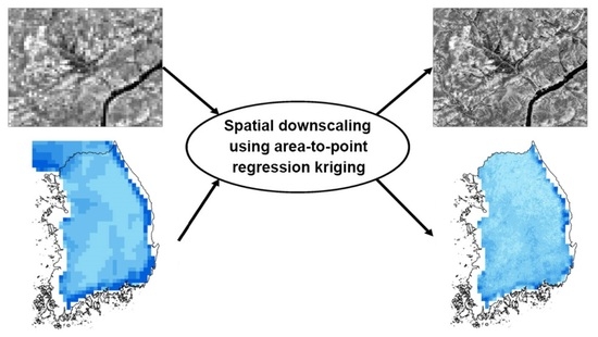
3.2. Spatial Downscaling of the SM Dataset

Table 6. Coefficient of determination (R²) values of three regression models for the SM dataset (unit: %).

Year	Month	LR	RF	SVR
2015	May	32.67	88.31	75.61
	June	46.59	91.69	84.22
	July	33.81	90.48	84.99
	August	30.57	89.68	91.87
	September	39.36	90.00	79.25
	October	6.24	85.56	83.26
2016	May	22.57	86.11	79.01
	June	44.82	90.68	76.79
	July	22.29	88.56	79.58
	August	28.02	88.53	82.20
	September	28.13	90.13	84.85
	October	28.21	90.80	90.45
2017	May	22.80	85.71	72.40
	June	46.88	89.90	69.28
	July	28.35	91.13	89.47
	August	17.09	86.85	89.22
	September	29.39	87.69	73.65
	October	14.06	89.34	87.75

shows the explanatory power of three regression models for TC estimation. Similar to the Landsat dataset, the highest R² value was obtained via RF across almost all months. LR achieved the lowest explanatory power and also showed very low R² values for some months (e.g., October 2015 and 2017). The R² values of LR and RF were negatively correlated with the mean of the actual observation values (−0.568 for both models), which means that auxiliary variables were insufficient to account for humid soil conditions. In contrast, SVR showed a positive correlation with the mean of observation values (0.591), which affected the predictive performance of the spatial downscaling results.

Table 7. Mean absolute error values of all comparison cases for the SM dataset. The best case per month is shown in bold. The case name can be referred to in Table 2.

Year	Month	Input	C1_LR	C1_RF	C1_SVR	C2_LR	C2_RF	C2_SVR	C3_RF	C3_SVR
2015	May	11.73	11.03	10.87	10.02	11.10	11.09	10.03	11.84	10.61
	Jun.	5.55	4.62	4.31	4.79	5.76	4.69	4.97	5.71	4.75
	Jul.	8.01	9.27	5.52	6.81	10.25	5.97	7.79	7.88	7.30
	Aug.	12.41	12.13	11.28	8.43	12.87	11.48	8.59	12.85	10.69
	Sep.	12.95	12.02	12.16	9.51	12.19	12.33	9.53	13.48	11.16
	Oct.	12.14	11.03	10.98	9.87	11.63	11.22	9.98	12.54	11.23
2016	May	14.67	14.63	14.42	14.30	14.21	14.21	13.91	14.47	14.18
	Jun.	7.75	7.90	6.65	6.23	8.18	6.78	6.29	7.76	6.87
	Jul.	13.62	12.70	10.89	9.37	13.47	11.38	9.99	13.06	11.91
	Aug.	9.46	9.62	7.90	6.10	10.42	8.43	6.18	9.83	8.18
	Sep.	14.64	12.09	12.84	9.26	13.26	12.95	9.29	15.06	12.87
	Oct.	16.07	14.91	14.29	12.76	16.16	14.29	12.81	16.31	14.78
2017	May	10.27	8.79	9.40	7.38	9.16	9.60	7.50	10.67	8.74
	Jun.	6.08	5.80	5.26	5.66	6.74	5.93	6.16	6.63	6.34
	Jul.	11.89	10.34	8.44	7.78	12.64	9.51	8.35	12.21	10.63
	Aug.	13.69	11.45	9.87	8.39	12.33	10.34	8.74	13.69	11.78
	Sep.	14.78	12.30	13.78	12.55	13.09	13.84	12.53	14.88	14.38
	Oct.	14.88	12.62	13.51	12.58	13.70	13.56	12.71	15.32	13.55

presents the MAE values of all comparison cases between 2015 and 2017. The accuracy values of the input AMSR-2 SM data are also presented to compare the impact of input errors on prediction accuracy. All cases showed negative mean error values (not shown here), which indicates an underestimation of the observation values. This underestimation resulted from the direct comparison of areal values with point observations, as well as the actual underestimation of satellite products. The TC estimates with SVR (C1_SVR) achieved the best prediction accuracy for most months (13 out of 18 months). This result is similar to the result of the Landsat dataset, that is, the TC estimates predicted well when the input data contained severe errors. The following best predictions were produced by the TC estimates with RF (3 out of 18 months). In most cases, LR-based ATPRK (C2_LR) and RF-based ATPRK with TC normalization (C3_RF) showed the worst accuracy. For example, C2_LR and C3_RF for August 2016 exhibited decreases of 86% and 61% in MAE, respectively, compared to the best case (C1_SVR). In particular, the MAE values of those predictions were worse than those of the input data, indicating that input errors were amplified after spatial downscaling.

The MRAE was found to be more effective than the MAE because it allowed for relative comparisons of SM values that vary over time. Figure 3 presents the variations of MRAE values for all comparison cases over the considered period. The superior prediction accuracy of C1_SVR is clearly shown over time. The next best prediction was obtained by C2_SVR (12 out of 18 months). It is noteworthy that the accuracy values of most predictions, except for C3_RF and C2_LR, were superior to those of input AMSR-2 data when considering that spatial downscaling aims to predict fine-scale attribute values, not to produce results with superior accuracy to the input coarse resolution data.

For the LR-based prediction, ATPRK had worse predictions than the TC estimate. When comparing three RF-based prediction results, the difference in MRAE between C1 and C3 was the largest. A relatively smaller difference was obtained between C1 and C2, indicating the lack of contribution of residual correction to the improvement in accuracy. Like the LR-based prediction, the accuracy of the TC estimation (C1) was better than the two ATPRK predictions (C2 and C3). Similar results were also observed for the SVR-based prediction. These results indicate that residual correction did not always improve prediction performance, particularly when the input data contained severe errors. Furthermore, ATPRK with the TC normalization degraded the prediction accuracy, compared to conventional ATPRK prediction.

The impacts of both the explanatory power of regression models and input errors on predictive performance were further analyzed using correlation coefficients between accuracy values, and R² and input errors were calculated for all prediction cases. All correlation coefficients between input errors and predictive accuracy values were statistically significant at the significance level of 1%. However, the correlation between accuracy and R² values was not significant at the significance level of 5%, except for LR-based predictions (C1_LR and C2_LR). Hence, only correlation coefficients between accuracy measures and errors of input SM data were considered (Figure 4).

Strong correlations were observed between the input errors and predictive accuracy for all cases (Figure 4). This result indicates that errors in input coarse resolution data greatly affect the quality of spatial downscaling results, like in the case of the Landsat dataset. Although there were no significant differences in correlation for the three regression models, RF-based ATPRK with TC normalization (C3_RF) showed the highest correlation coefficient value (0.996 for MAE and 0.990 for MRAE). Other RF-based predictions (C2_RF and C1_RF) also had strong correlations to input errors, which implies that RF-based predictions are most susceptible to input errors. In contrast, the prediction accuracy values of C1_SVR and C2_SVR showed the lowest correlation to the input errors. Consequently, C1_SVR achieved the best prediction accuracy for most cases.

Despite the insignificance of the correlation between accuracy and R² values, a further interpretation was made. The moderately negative correlation between the accuracy values of LR-based predictions and the R² values (−0.59 and −0.61 for C1_LR and C2_LR, respectively) indicates that the higher explanatory power of TC estimation may lead to a slight improvement in accuracy. In addition, as shown in Table 6, a positive correlation of the R² value of SVR to the mean of the observations might contribute to better prediction performance, particularly in the summer season. However, as found in the Landsat dataset, the highest R² values of RF in most cases did not lead to better prediction accuracy. Furthermore, TC estimation with very low explanatory power showed worse prediction accuracy.

Based on the results of the experiment on the real SM dataset, it can be concluded that the use of the TC estimate as a downscaling result exhibited the best prediction performance. In addition, as input errors increased, prediction errors increased accordingly. A clear correlation between the explanatory power of regression models and prediction accuracy was not observed. However, it is evident that higher explanatory power cannot always guarantee improvement in prediction accuracy.

4. Discussion and Conclusions

The main contribution of this study lies in exploring the variations in the predictive performance of different TC estimations to different input errors in ATPRK-based spatial downscaling. To fill the gap from previous studies based on a single attribute and/or a small number of data [26,27], the sensitivity analysis in this study was based on extensive comparisons using synthetic and real datasets. As error information of real satellite-derived products is usually unavailable, a direct comparison of results from the real dataset may not be compatible with those from the synthetic dataset with known errors. Despite the limitation of using error information from a limited number of actual observation sites in the real SM dataset, common results could be derived from the two experimental datasets in this study.

The results from two experiments indicate that the quality of the spatial downscaling result depends heavily on the accuracy of input data. When input data become more erroneous, the prediction accuracy decreases accordingly. For input data with no or few errors, residual correction is recommended to improve the prediction accuracy. TC normalization is also effective when nonlinear regression models are employed for TC estimation. However, in spatial downscaling of coarse resolution data with significant errors (i.e., SM dataset in this study), residual correction and TC normalization cannot achieve better prediction performance, and the use of TC estimate as a prediction result is more effective. These findings were not reported in most spatial downscaling studies where input errors were not considered in spatial downscaling of satellite-derived products [16,17,18,19]. When noisy coarse resolution data are used as input for spatial downscaling, the RCs that remain after regression modeling inevitably include input errors, depending on the explanatory power of the applied regression model. As a result, the errors of the coarse resolution RCs propagate to the ATPK-based RC predictions. In addition, the TC normalization procedure aiming at reproducing the patterns of the erroneous input data also yields a worse result.

As found in the previous study [26], the higher explanatory power of regression modeling for TC estimation does not always lead to better prediction accuracy. When downscaling the coarse resolution data with significant errors (the SM dataset in this study), the prediction accuracy was not clearly correlated to the explanatory power. Instead, the regression model with higher explanatory power (RF in this study) predicted worse than other modes with relatively lower explanatory power. Quantitative relationships modeled at a coarse resolution are directly applied to auxiliary variables at a fine resolution for the TC estimation. Thus, a possible explanation for the worse prediction in the case with higher explanatory power is that the relationships at a coarse resolution distorted by overfitting to the noisy input (too higher R² values) are likely to generate erroneous TC estimates at a fine resolution. It should be noted that the superiority of SVR to LR and RF in this study does not indicate that SVR is an optimal TC estimator in spatial downscaling. Instead, using the magnitude of explanatory power in the TC estimation as a direct indicator to select an optimal regression model requires caution, particularly when the input data contain errors. Recently, geographically weighted regression (GWR) has often been applied in ATPRK-based spatial downscaling [35,36,37]. As regression coefficients are estimated locally, the explanatory power of GWR is likely to be higher than that of other regression models. As a result, GWR may be more susceptible to input errors than other models in some cases. Therefore, it is worthwhile to analyze the impact of input errors on the predictive performance of GWR-based spatial downscaling to confirm the results of this study.

In future work, an advanced procedure to account for input errors during spatial downscaling should be developed to improve predictive performance in spatial downscaling of coarse resolution data with errors. From a methodological viewpoint, filtered kriging, as proposed by Christensen [38], can be applied to filter out noise or errors in coarse resolution satellite-derived products when error variance information is available. Then, the noise-filtered coarse resolution data can be used as input for ATPRK-based spatial downscaling. The main difficulty of this approach is in the availability of error information. Unlike the synthetic dataset, however, the error information of satellite-based products is usually not available in the study area of interest. When sufficient ground observation data are available, they can be used to generate error distribution maps through geostatistical simulation [39]. The potential of this approach for error filtering should be explored in future work.

As new satellite operation programs continue to be developed, many satellite-based products are expected to be available in the future. However, it is not always possible to obtain satellite data acquired at the desired spatial resolution. Thus, spatial downscaling will remain vital in satellite data reconstruction. Based on the major findings and recommendations from this study, spatial downscaling results with improved quality can effectively provide thematic information for environmental monitoring and modeling.

References

1. Ghamisi, P.; Rasti, B.; Yokoya, N.; Wang, Q.; Höfle, B.; Bruzzone, L.; Bovolo, F.; Chi, M.; Anders, K.; Gloaguen, R.; et al. Multisource and multitemporal data fusion in remote sensing: A comprehensive review of the state of the art. IEEE Geosci. Remote Sens. Mag. 2019, 7, 6–39. [Google Scholar] [CrossRef]
2. Park, N.-W.; Kim, Y.; Kwak, G.-H. An overview of theoretical and practical issues in spatial downscaling of coarse resolution satellite-derived products. Korean J. Remote Sens. 2019, 35, 589–607. [Google Scholar]
3. Sdraka, M.; Papoutsis, I.; Psomas, B.; Vlachos, K.; Ioannidis, K.; Karantzalos, K.; Gialampoukidis, I.; Vrochidis, S. Deep learning for downscaling remote sensing images: Fusion and super-resolution. IEEE Geosci. Remote Sens. Mag. 2022, 10, 202–255. [Google Scholar] [CrossRef]
4. Atkinson, P.M. Downscaling in remote sensing. Int. J. Appl. Earth Obs. Geoinf. 2013, 22, 106–114. [Google Scholar]
5. Immerzeel, W.W.; Rutten, M.M.; Droogers, P. Spatial downscaling of TRMM precipitation using vegetation response on the Iberian Peninsula. Remote Sens. Environ. 2009, 113, 362–370. [Google Scholar] [CrossRef]
6. Jia, S.; Zhu, W.; Lü, A.; Yan, T. A statistical spatial downscaling algorithm of TRMM precipitation based on NDVI and DEM in the Qaidam Basin of China. Remote Sens. Environ. 2011, 115, 3069–3079. [Google Scholar] [CrossRef]
7. Sachindra, D.A.; Ahmed, K.; Rashid, M.M.; Shahid, S.; Perera, B.J.C. Statistical downscaling of precipitation using machine learning techniques. Atmos. Res. 2018, 212, 240–258. [Google Scholar] [CrossRef]
8. Shen, Z.; Yong, B. Downscaling the GPM-based satellite precipitation retrievals using gradient boosting decision tree approach over Mainland China. J. Hydrol. 2021, 602, 126803. [Google Scholar] [CrossRef]
9. Yan, X.; Chen, H.; Tian, B.; Sheng, S.; Wang, J.; Kim, J.-S. A downscaling–merging scheme for improving daily spatial precipitation estimates based on random forest and cokriging. Remote Sens. 2021, 13, 2040. [Google Scholar] [CrossRef]
10. Kofidou, M.; Stathopoulos, S.; Gemitzi, A. Review on spatial downscaling of satellite derived precipitation estimates. Environ. Earth Sci. 2023, 82, 424. [Google Scholar] [CrossRef]
11. Choi, M.; Hur, Y. A microwave-optical/infrared disaggregation for improving spatial representation of soil moisture using AMSR-E and MODIS products. Remote Sens. Environ. 2012, 124, 259–269. [Google Scholar] [CrossRef]
12. Jin, Y.; Ge, Y.; Wang, J.; Chen, Y.; Heuvelink, G.B.M.; Atkinson, P.M. Downscaling AMSR-2 soil moisture data with geographically weighted area-to-area regression kriging. IEEE Trans. Geosci. Remote Sens. 2018, 56, 2362–2376. [Google Scholar] [CrossRef]
13. Wei, Z.; Meng, Y.; Zhang, W.; Peng, J.; Meng, L. Downscaling SMAP soil moisture estimation with gradient boosting decision tree regression over the Tibetan Plateau. Remote Sens. Environ. 2019, 225, 30–44. [Google Scholar] [CrossRef]
14. Zhao, H.; Li, J.; Yuan, Q.; Lin, L.; Yue, L.; Xu, H. Downscaling of soil moisture products using deep learning: Comparison and analysis on Tibetan Plateau. J. Hydrol. 2022, 607, 127570. [Google Scholar] [CrossRef]
15. Nadeem, A.A.; Zha, Y.; Shi, L.; Ali, S.; Wang, X.; Zafar, Z.; Afzal, Z.; Tariq, M.A.U.R. Spatial downscaling and gap-filling of SMAP soil moisture to high resolution using MODIS surface variables and machine learning approaches over ShanDian River Basin, China. Remote Sens. 2023, 15, 812. [Google Scholar] [CrossRef]
16. Hutengs, C.; Vohland, M. Downscaling land surface temperatures at regional scales with random forest regression. Remote Sens. Environ. 2016, 178, 127–141. [Google Scholar]
17. Bartkowiak, P.; Castelli, M.; Notarnicola, C. Downscaling land surface temperature from MODIS dataset with random forest approach over Alpine vegetated areas. Remote Sens. 2019, 11, 1319. [Google Scholar] [CrossRef]
18. Yoo, C.; Im, J.; Park, S.; Cho, D. Spatial downscaling of MODIS land surface temperature: Recent research trends, challenges, and future directions. Korean J. Remote Sens. 2020, 36, 609–626. [Google Scholar]
19. Ouyang, X.; Dou, Y.; Yang, J.; Chen, X.; Wen, J. High spatiotemporal rugged land surface temperature downscaling over Saihanba Forest Park, China. Remote Sens. 2022, 14, 2617. [Google Scholar] [CrossRef]
20. Liang, M.; Zhang, L.; Wu, S.; Zhu, Y.; Dai, Z.; Wang, Y.; Qi, J.; Chen, Y.; Du, Z. A high-resolution land surface temperature downscaling method based on geographically weighted neural network regression. Remote Sens. 2023, 15, 1740. [Google Scholar] [CrossRef]
21. Wang, Q.; Shi, W.; Atkinson, P.M.; Zhao, Y. Downscaling MODIS images with area-to-point regression kriging. Remote Sens. Environ. 2015, 166, 191–204. [Google Scholar] [CrossRef]
22. Wang, Q.; Shi, W.; Li, Z.; Atkinson, P.M. Fusion of Sentinel-2 images. Remote Sens. Environ. 2016, 187, 241–252. [Google Scholar] [CrossRef]
23. Vaithiyanathan, D.; Sudalaimuthu, K. Area-to-point regression kriging approach fusion of Landsat 8 OLI and Sentinel 2 data for assessment of soil macronutrients at Anaimalai, Coimbatore. Environ. Monit. Assess. 2022, 194, 916. [Google Scholar] [CrossRef] [PubMed]
24. Zhang, Y.; Atkinson, P.M.; Ling, F.; Foody, G.M.; Wang, Q.; Ge, Y.; Li, X.; Du, Y. Object-based area-to-point regression kriging for pansharpening. IEEE Trans. Geosci. Remote Sens. 2021, 59, 8599–8614. [Google Scholar] [CrossRef]
25. Tziokas, N.; Zhang, C.; Drolias, G.C.; Atkinson, P.M. Downscaling satellite night-time lights imagery to support within-city applications using a spatially non-stationary model. Int. J. Appl. Earth Obs. Geoinf. 2023, 122, 103395. [Google Scholar] [CrossRef]
26. Kim, Y.; Park, N.-W. Impact of trend estimates on predictive performance in model evaluation for spatial downscaling of satellite-based precipitation data. Korean J. Remote Sens. 2017, 33, 25–35. [Google Scholar] [CrossRef]
27. Kim, Y.; Park, N.-W. Assessing the impacts of errors in coarse scale data on the performance of spatial downscaling: An experiment with synthetic satellite precipitation products. Korean J. Remote Sens. 2017, 33, 445–454. [Google Scholar]
28. Kyriakidis, P.C. A geostatistical framework for area-to-point spatial interpolation. Geogr. Anal. 2004, 36, 259–289. [Google Scholar] [CrossRef]
29. Wang, Q.; Shi, W.; Atkinson, P.M. Area-to-point regression kriging for pan-sharpening. ISPRS J. Photogramm. Remote Sens. 2016, 114, 151–165. [Google Scholar] [CrossRef]
30. Breiman, L. Random forests. Mach. Learn. 2001, 45, 5–32. [Google Scholar] [CrossRef]
31. Hultquist, C.; Chen, G.; Zhao, K. A comparison of Gaussian process regression, random forests and support vector regression for burn severity assessment in diseased forests. Remote Sens. Lett. 2014, 5, 723–732. [Google Scholar] [CrossRef]
32. Moser, G.; Serpico, S.B. Automatic parameter optimization for support vector regression for land and sea surface temperature estimation from remote sensing data. IEEE Trans. Geosci. Remote Sens. 2009, 47, 909–921. [Google Scholar] [CrossRef]
33. Scikit-Learn: Machine Learning in Python. Available online: https://scikit-learn.org (accessed on 14 July 2023).
34. Agrometeorological Information Service. Available online: http://weather.rda.go.kr/w/index.do (accessed on 3 July 2023).
35. Jin, Y.; Ge, Y.; Wang, J.; Heuvelink, G.B.M.; Wang, L. Geographically weighted area-to-point regression kriging for spatial downscaling in remote sensing. Remote Sens. 2018, 10, 579. [Google Scholar] [CrossRef]
36. Wen, F.; Zhao, W.; Wang, Q.; Sánchez, N. A value-consistent method for downscaling SMAP passive soil moisture with MODIS products using self-adaptive window. IEEE Trans. Geosci. Remote Sens. 2020, 58, 913–924. [Google Scholar] [CrossRef]
37. Li, N.; Wu, H.; Ouyang, X. Localized downscaling of urban land surface temperature—A case study in Beijing, China. Remote Sens. 2022, 14, 2390. [Google Scholar] [CrossRef]
38. Christensen, W.F. Filtered kriging for spatial data with heterogeneous measurement error variances. Biometrics 2011, 67, 947–957. [Google Scholar] [CrossRef] [PubMed]
39. Park, N.-W.; Kyriakidis, P.C. A geostatistical approach to spatial quality assessment of coarse spatial resolution remote sensing products. J. Sens. 2019, 2019, 7297593. [Google Scholar] [CrossRef]
Figure 1. Workflow of ATPRK for spatial downscaling with fine resolution auxiliary variables.
Applsci 13 10233 g001
Figure 2. Two datasets used for spatial downscaling experiments: (a) Landsat shortwave infrared band image; (b) AMSR-2 soil moisture data in July 2017 (unit: %). The black polylines and dots in (b) denote the administrative boundary of South Korea and soil moisture observation sites used for accuracy evaluation, respectively.
Applsci 13 10233 g002
Figure 3. The radar chart of mean relative absolute errors for all spatial downscaling results for the SM dataset. The case name can be referred to in Table 2.
Applsci 13 10233 g003
Figure 4. Correlation coefficients between accuracy measures and input errors. The case name can be referred to in Table 2.
Applsci 13 10233 g004