1. Introduction
Hypersonic vehicles generally refer to vehicles with a Mach number greater than 5, which can travel in near space or across the atmosphere, including hypersonic missiles, hypersonic manned or unmanned aircraft and space vehicles. Hypersonic vehicles are of great military strategic significance and commercial value, due to their fast flight speed, difficulty in detection and interception, and the ability to achieve long-range rapid strikes against enemy targets. Hypersonic flight has become one of the critical technologies that the world’s space powers are competing for [
1]. Presently, many countries are highly interested in the domain of near space and are accelerating the development of various hypersonic vehicles.
Although the great potentials of hypersonic vehicles for military strategy and space exploration are well recognized, there remain many “unaware unknowns” or “aware unknowns” [
2] that need to be solved, such as “blackout” [
3] and “thermal barrier” [
4]. The space shuttle Columbia crashed in a severe aerodynamic thermal environment during its reentry from orbit in 2003 [
2], leading to the recognition that the study of aerodynamic heating is a critical problem that cannot be bypassed on the road of hypersonic flight.
When the hypersonic vehicle flies at very high speed in atmosphere, a strong bow shock wave forms around the blunt nose of the vehicle due to the sharp compression of air. The flow temperature behind the shock can exceed thousands or even 10,000 K, resulting in the severe aerodynamic heating to the vehicle as well as the excitations of internal energy modes, dissociation and ionization reactions of air species. The air ionization generates the plasma to intervene with the electromagnetic wave transmission, which leads to the communication signal interruption, that is “blackout” [
5]. In fact, the excitation of internal energy modes and chemical reactions of air species do not occur independently and are always intercoupling. For example, the molecules in the high vibrational level prefer to dissociate, while the dissociation reaction leads to the loss of total vibrational energy [
6]. In the meantime, when the characteristic times of the relaxations of internal energy excitation or chemical reactions reach comparable level to the characteristic time of flow, there are thermochemical nonequilibrium effects, which can greatly affect the aerothermodynamic environment of the hypersonic vehicle. Therefore, it is very important to predict the thermochemical nonequilibrium processes accurately for the design of hypersonic vehicle [
7].
However, limited to the operation cost and technical conditions, it is still very difficult to reproduce the high-temperature and high-enthalpy environment of real hypersonic flight on the ground. Therefore, numerical simulation becomes an indispensable technique for evaluating the aerothermodynamic properties of the hypersonic flow. Until now, many different thermodynamic and chemical kinetic models have been developed by Park [
8,
9], Gupta et al. [
10], Dunn and Kang [
11] to calculate the thermochemical nonequilibrium effects in the hypersonic flow, which have become the foundations of the related numerical studies over decades. Jiang et al. [
12] investigated the hypersonic shock wave/turbulent boundary layer interaction with the thermochemical nonequilibrium effects using the Park’s two-temperature model and Gupta 11-species model. The results showed that the combined effect of turbulence and thermochemical nonequilibrium has a significant impact on the flow structure, wall characteristic and separation length of the shock/boundary layer interaction. By comparing the effects of Dunn-Kang, Gupta, Park 87 and Park 91 chemical kinetic models on the hypersonic aerodynamic heating, Wang et al. [
13] found that the heat flux on the surface of a vehicle with the complex shape is more sensitive to the choice of chemical reaction model, and the maximum difference of the peak heat flux may exceed 25%. Dong et al. [
14] used the Dunn-Kang 5-species, 7-species, 11-species chemical reaction models and one-temperature, two-temperature thermodynamic models to solve the thermochemical nonequilibrium flow, respectively, and found that the differences between the heat flux distributions predicted by the 7-and 11-species was not significant, while the heat flux of the 5-species was smaller, with a difference up to 10% or even more; the heat fluxes calculated by different thermodynamic models are slightly different, with a maximum difference of about 10%. Zhao et al. [
15] compared the aerodynamic heat fluxes under the Gupta 5-, 7-, 11-species chemical reaction models and found that the wall heat fluxes under the 7- and 11-species were significantly larger than that of the 5-species when the Mach number was greater than 12, and that the 7-species model should be adopted. Dobrov et al. [
16] used the Gupta 5-species and Park 5-species chemical kinetic models to solve the nearly same results of the air compositions at the stagnation point of a sphere. However, the difference between the shock standoff distances calculated with perfect gas and chemical reaction gas is significant. Mo et al. [
17] analyzed the effects of the physicochemical models by solving high temperature chemical nonequilibrium flow, and found that the commonly used chemical kinetic model of Gupta generally calculates the larger shock standoff distance than the models of Dunn-Kang and Park. For complex flow regions such as the shock/shock interaction, the difference between the predicted peak heat flux using different chemical kinetic models is up to 20% or even more. The application of different models results in differences in aerodynamic predictions, which causes confusion in model selection when calculating hypersonic nonequilibrium flow.
Above all, previous studies have suggested that a systematic evaluation should be conducted to investigate the combined effects of different thermodynamic and chemical kinetic models commonly used for simulating the hypersonic thermochemical nonequilibrium flow in a comprehensive and detailed way. In this paper, the HyFLOW software [
18] is employed to solve the hypersonic thermochemical nonequilibrium flows around a standard cylinder to compare the effects of different thermodynamic models (one- and two-temperature models) respectively with different chemical kinetic models of air (Park 5-species, 7-species, 11-species; Gupta 5-species, 7-species, 11-species; Dunn-Kang 5-species, 7-species, 11-species) on the aerodynamic characteristics, and in the meantime, to investigate whether the reduced models can be used instead of the complex models under certain conditions, for achieving a balance between computational efficiency and computational accuracy.
This study firstly summarizes the previous research work and presents the purpose, significance and research methodology of this paper. Secondly, it introduces the mathematical and physical models in detail, including the governing equations, thermochemical nonequilibrium source terms, transport properties, and the HyFLOW software. Then, it shows the hypersonic thermochemical nonequilibrium flow results solved by different model combinations and analyzes the effects of different models on the flow temperature, pressure, shock standoff distance, and wall heat flux. Finally, the conclusions are made.
2. Mathematical and Physical Models
Table 1 lists two different thermodynamic models and three chemical kinetic models commonly used in the previous studies to characterize the internal energy excitations and the chemical reactions of air species. Every chemical kinetic model contains three models with different number of components, they are 5-species (N
2, O
2, N, O, NO), 7-species (N
2, O
2, N, O, NO, NO
+, e
−), and 11-species (N
2, O
2, N, O, NO, NO
+, e
−,
,
, N
+, O
+). Any one thermodynamic model together with any one chemical reaction model of 5-, 7- or 11-species can be chosen from
Table 1 to calculate the thermochemical nonequilibrium effects for the hypersonic flow simulation, and thus there are eighteen combinations in all for comparison. For the two-temperature model,
Ttr represents the equilibrium temperature corresponding to the translational energy mode and the rotational energy mode, and
Tve corresponds to the equilibrium temperature of the vibrational energy mode and the electronic energy mode; The one-temperature model indicates that all the internal energy modes are equilibrated in one temperature, that is
Ttr =
Tve =
T. In the present study, the governing equations of hypersonic flow are still based on the Navier-Stokes (N-S) equations under the continuum assumption, closed with the models of source terms and transport properties.
2.1. Governing Equations
The system of the N-S equations for the hypersonic thermochemical nonequilibrium flow are given as follows:
The species continuum equations:
and the total density is
The total energy equation for the one-temperature model:
The total energy equation for the two-temperature model:
The vibrational-electronic energy equation for the two-temperature model:
where
Ns is the total number of gas mixture components;
ρs,
eves,
hs,
Ys and
Ds are the density, vibrational-electronic energy, specific enthalpy, mass fraction and mass diffusion coefficient of the
s-th component, respectively;
uj denotes the
j directional flow rate;
eve,
e and
h denote the vibrational-electronic energy, total specific energy and total specific enthalpy,
T is the temperature,
ρ is the total density,
Ttr and
Tve are translational-rotational temperature and vibrational-electronic temperature,
P and
τij are the pressure and molecular viscous stress respectively;
ωve,
ωs are the vibrational-electronic energy source term and the
s component chemical reaction generation source term respectively, and the radiation source term can be neglected in this paper;
k,
ktr and
kve correspond to the total thermal conductivity, the thermal conductivity of the translational-rotational temperature and the vibrational-electronic temperature respectively.
2.2. Chemical Reaction Models
For the chemical reactions of air species in high temperature, the 5-, 7-, and 9-species models proposed by Gupta et al., Park and Dunn & Kang are all used in this study, the specific reaction equations and rate coefficients of which have been detailedly given in Refs. [
9,
10,
11], respectively.
The chemical reactions of the high temperature air can be generally written as:
where
As is the chemical formula of the component
s;
γrs and
are the stoichiometric coefficient of component
s for the forward and backward reactions, respectively;
Nr is the number of the chemical reactions. According to the law of mass action, the reaction rate of the chemical reaction
r is expressed as:
where
kfr and
kfb are the forward and backward reaction rate coefficients for the chemical reaction
r, respectively.
In the Dunn-Kang model, the forward and backward reaction rates are calculated using the Arrhenius law as follows:
where the subscripts ‘
f’ and ‘
b’ represents the forward and backward reactions;
A,
B and
C are the coefficients of the frequency factor, temperature index and activation temperature, respectively, which can be found in Ref. [
11].
In the Park model, the forward reaction rate coefficient is calculated by the Arrhenius law, while the backward reaction rate coefficient is calculated by the following equation:
where
Keq is the equilibrium constant, which can be obtained by the temperature fitting relation [
8]:
The chemical reaction source term in Equation (1) can be expressed as:
2.3. Vibrational-Electronic Energy Equation Source Term
The vibrational-electronic energy source term
ωve, which appears in Equation (6), is obtained by adding the vibrational energy source term and the electronic energy source term
The vibrational energy source term
ωv considers the following three terms: (i) the energy exchange between translational and vibrational modes, (ii) the energy exchange between electronic and vibrational modes and (iii) the vibration energy gained and lost due to molecular dissociation and atomic recombination in the cell [
19]. Thus,
where
evs,
,
are vibrational energy perunit mass of species
s, the vibrational energy perunit mass of species
s evaluated at temperature
T and electronic temperature
Te separately;
τvs,
τes are electronic-vibrational and translational-vibrational energy relaxation time for molecular species
s. The average vibrational energy perunit mass of molecule species
s Ds is created or destroyed at rate
ωs.
And the electronic energy source term
ωe considers the following three terms: (i) the energy exchange between heavy particles and electrons in translational modes, (ii) the energy exchange between vibration and electronic modes and (iii) the electronic energy gain and loss due to forced ionization reactions. Thus,
where
νes is effective collision frequency between the electron and the heavy particle of the
s component;
IO and
IN are molar first-order ionization energy of oxygen (O) and nitrogen (N) atoms, respectively;
RO and
RN represent the positive reaction rates of the O and N forced ionization reactions, respectively.
2.4. Transport Properties
2.4.1. Viscosity
The dynamic viscosity of the gas mixture is obtained by the Wilke’s semi-empirical formula [
20] as follows:
where
Xj,
Mj and
μj are the molar fraction, molar mass and dynamic viscosity of the component
j respectively;
is the average molar mass of the gas mixture. When the temperature is below 1000 K, the dynamic viscosity of each species is calculated by the Sutherland formula [
21]; while the temperature is higher than 1000 K, the component viscosity is obtained by Blottner temperature-fitting relation [
22,
23].
2.4.2. Mass Diffusion Coefficient
The mass diffusion coefficient of component
s is computed by
where
Sc is the Schmidt number and is taken as 0.5.
2.4.3. Thermal Conductivity
Total thermal conductivity of the gas mixture can be calculated by the following expression as:
The thermal conductivities
ktrs,
kvs, and
kes corresponding to the different internal energy modes are treated by the Eucken semi-empirical relation [
10].
2.5. HyFLOW
HyFLOW [
18] is a CFD software for the hypersonic flow simulation developed by the National Numerical Wind Tunnel (NNW) project and its basic framework is provided by the PHengLEI open source software. HyFLOW can solve the hypersonic flow including the thermochemical nonequilibrium effects and aero-physical properties of the high temperature of gas mixtures, and can also accurately predict the aerodynamic forces and heating of the hypersonic vehicle.
3. Results and Discussions
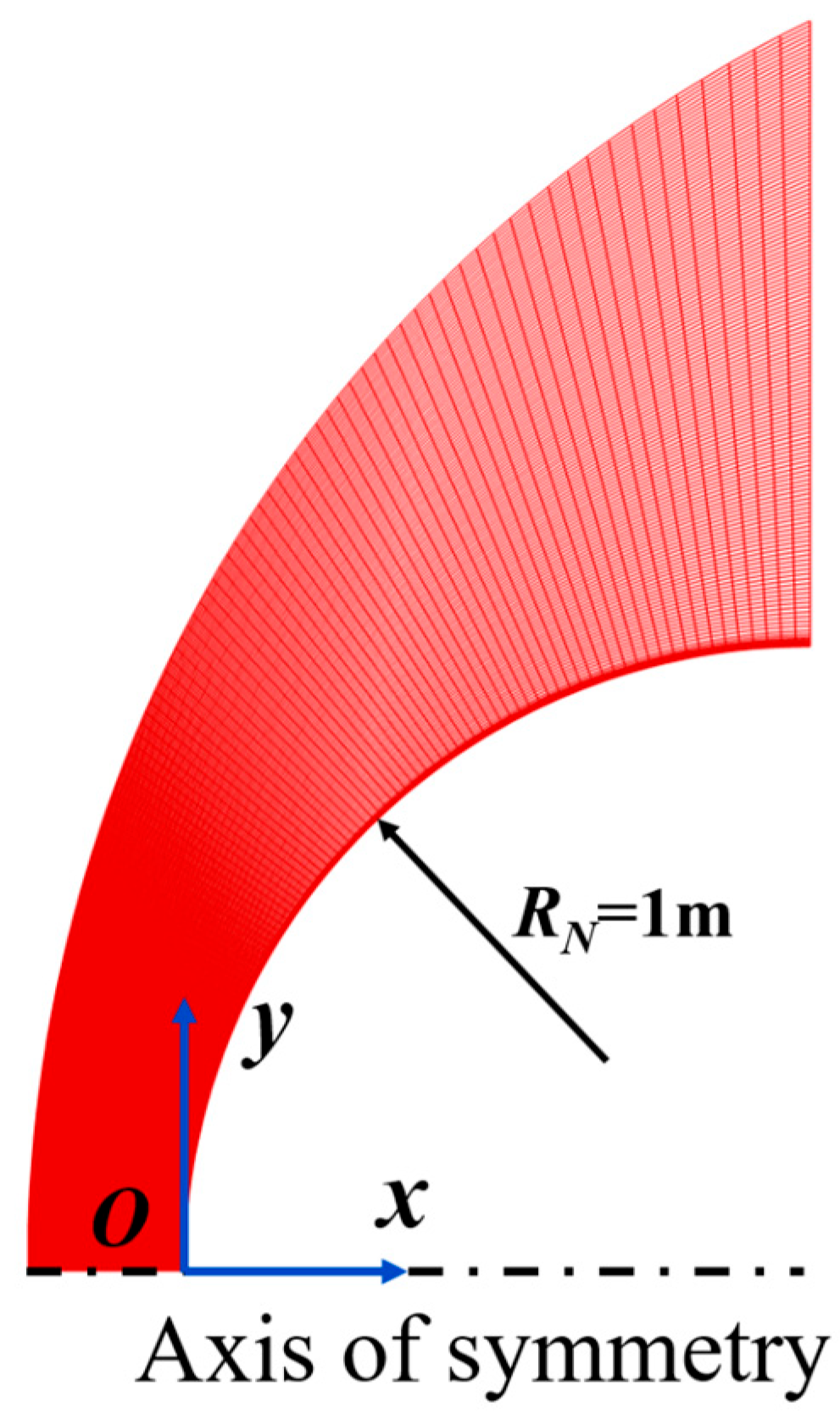
In this study, the hypersonic flow over a standard cylinder with the radius of 1 m is solved by HyFLOW to compare the effects of different chemical kinetic models and different temperature models. Three freestream conditions are taken from the real flight trajectory of FIRE II [
24] for simulation as shown in
Table 2, where
V∞ and
Ma are the freestream speed and Mach number,
ρ∞,
p∞ and
T∞ are the freestream density pressure and temperature, and
Tw is the wall temperature. Non-catalytic wall condition is used in this study. As list in
Table 1, different thermodynamic models together with different chemical kinetic models are employed to simulate the hypersonic flow around the cylinder for comparison, respectively, that is 18 model combinations in all. Additionally, all three cases are also solved using the perfect gas model as the baseline references. The mesh of the flow domain is 131 (along the wall) × 151 (normal to the wall), as shown in
Figure 1, and the spacing of the first grid layer to the wall is 1 × 10
−5 m.
3.1. Temperature
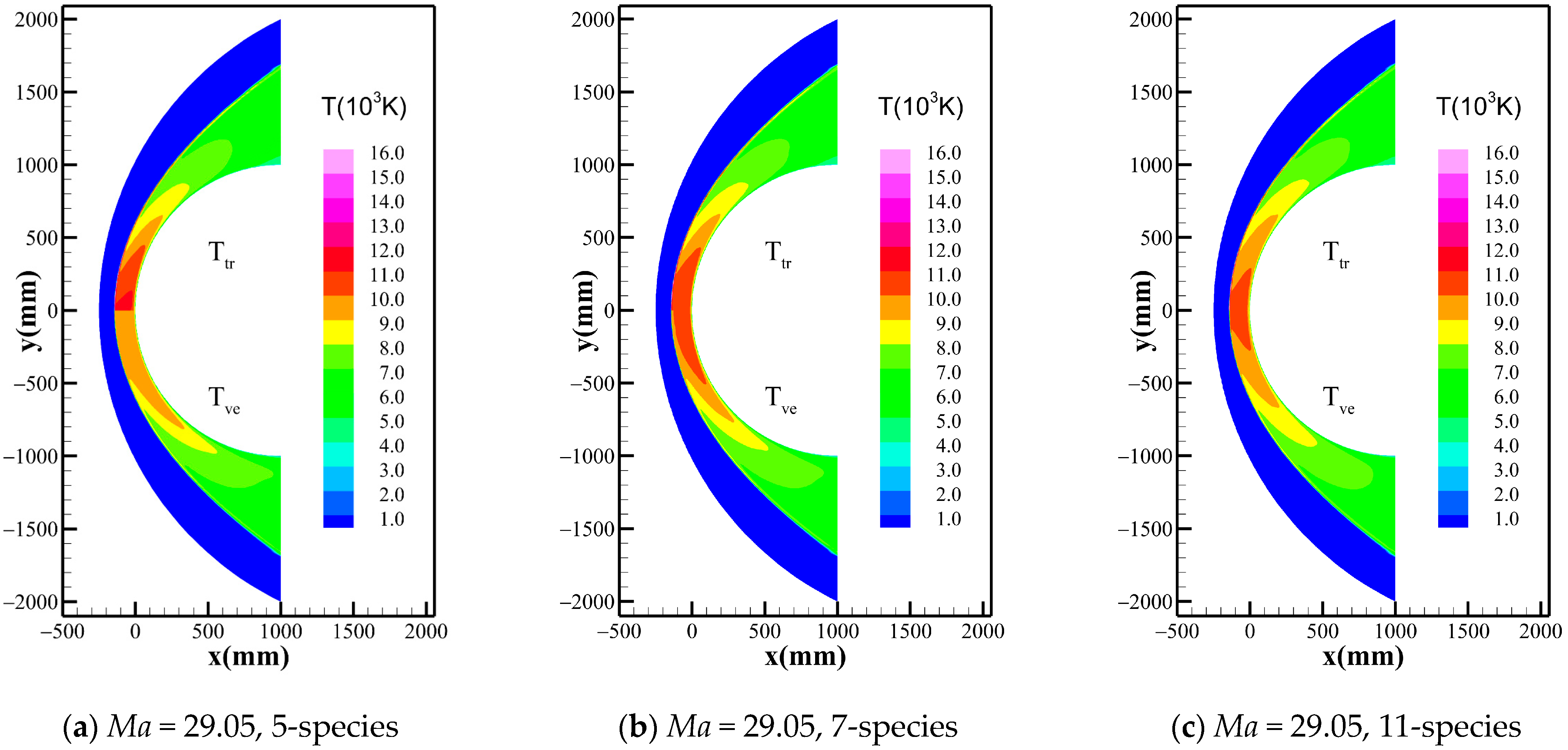
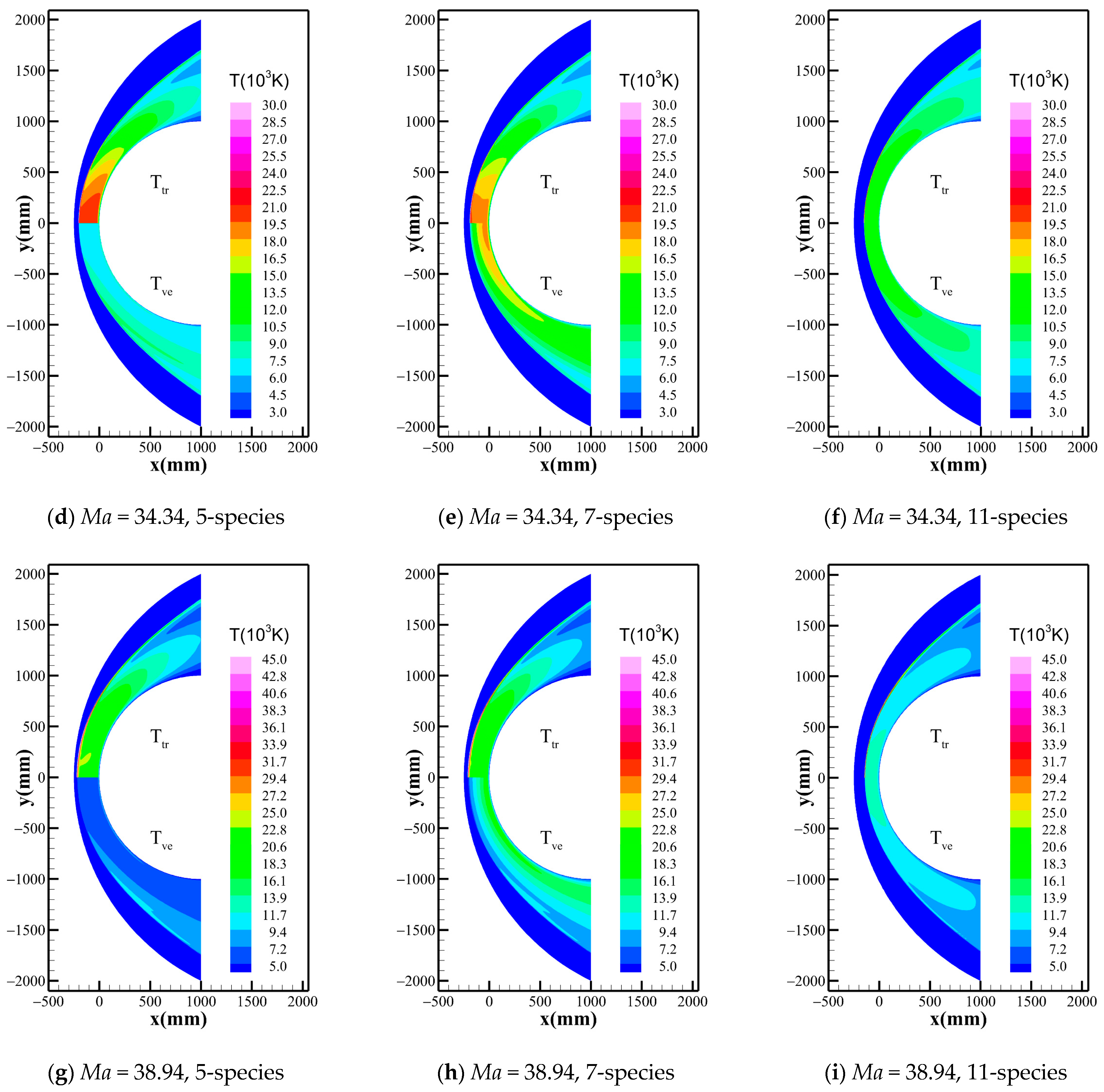
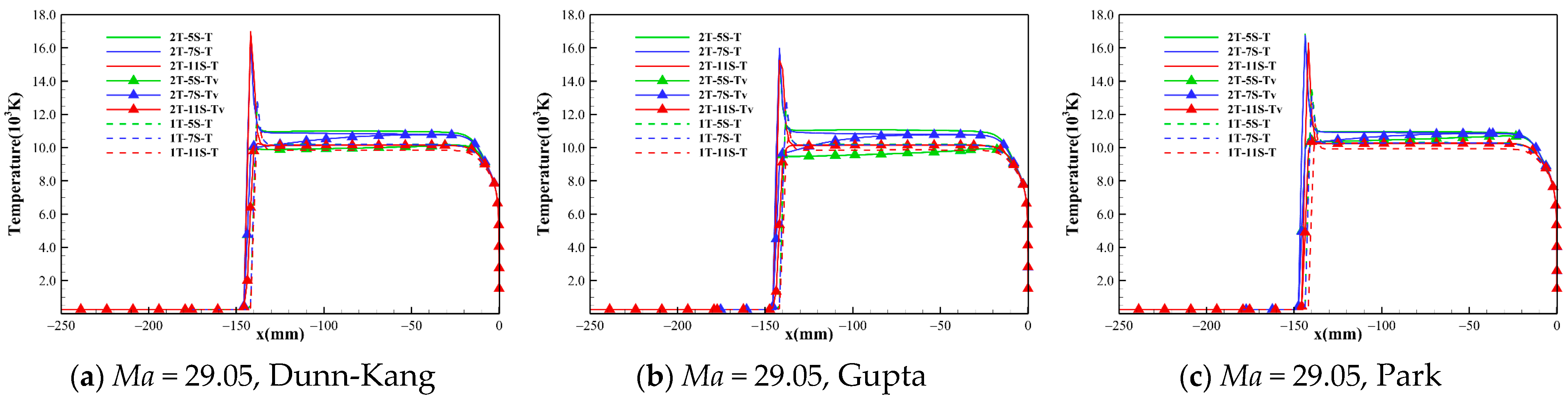
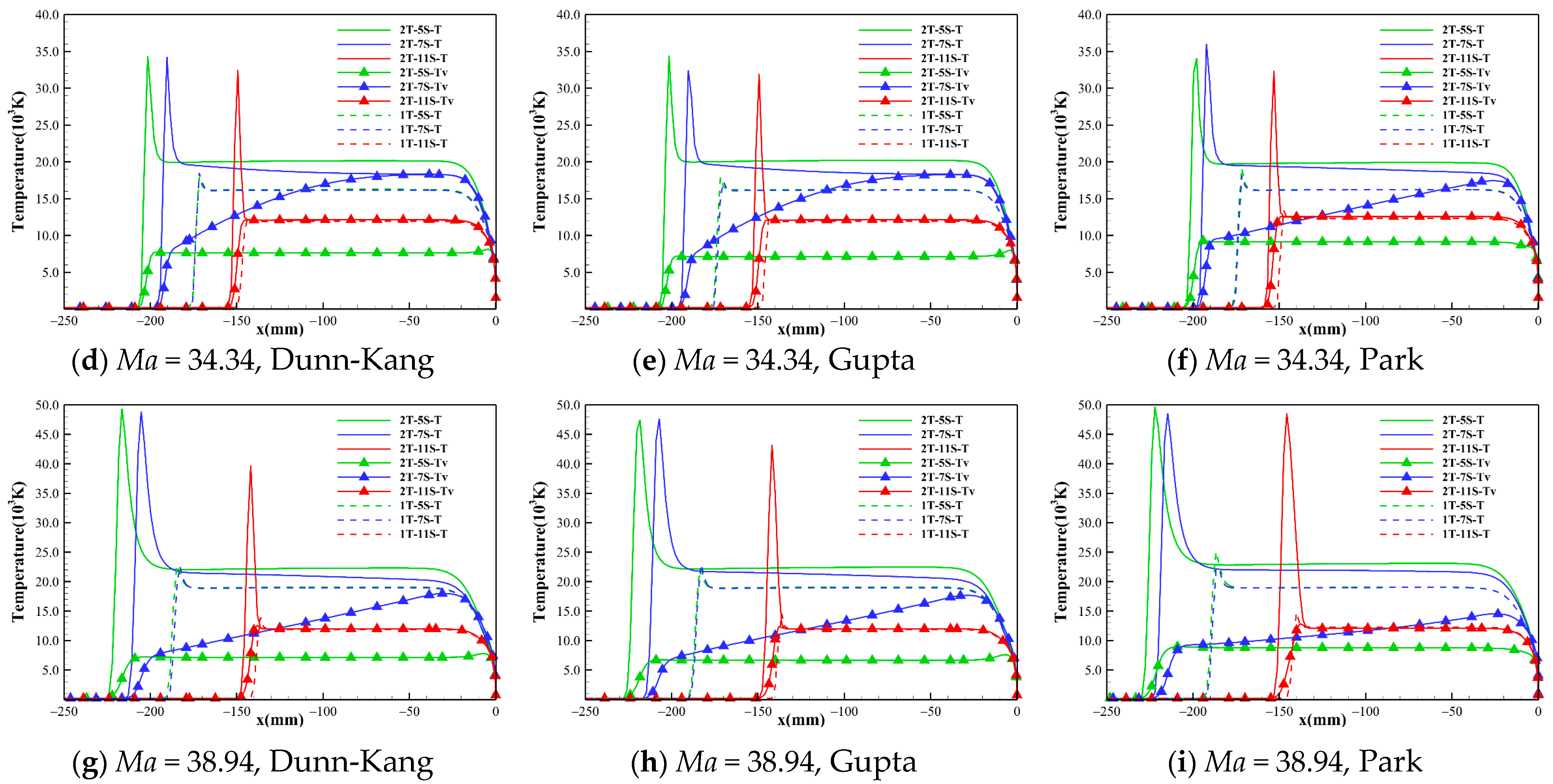
Figure 2 shows the temperature distribution of the flow field when Gupta 5-, 7-, and 11-species chemical reaction models are used at the three freestream conditions. It can be found that the peak temperatures of the flow field exceed 10,000 K in the shock layer for all three cases, and the translational-rotational and vibrational-electronic temperatures are highly unequal within a distance behind the shock, due to the existence of a significant thermochemical nonequilibrium effect. However, the differences between different chemical kinetic models rise gradually as the altitude and Mach number increase. To show more details, the temperature distribution along the stagnation line given by the 5-, 7-, and 11-species models of Dunn-Kang, Gupta, and Park combined with the two temperature models are shown in
Figure 3, respectively. The comparison of different chemical kinetic models reveals that the total number of gas species has a remarkable effect on both the peak and equilibrium temperatures inside the shock layer. Meanwhile, the thermodynamic nonequilibrium states in the flow field are also inconsistent between different model combinations, mainly affected by the total number of gas species. For 11-species model, the extremely high temperature behind the shock promotes the rapid exchange of energy among various modes, including the excitation of the vibrational energy modes of molecules, and the thermodynamic equilibrium quickly reaches in a very short distance. For 7-species model, thermodynamic nonequilibrium exists in most area of the shock layer, and the thermodynamic equilibrium just appears near the wall; For 5-species model, thermodynamically frozen flow occurs in most regions of the shock layer.
The temperature distribution along the stagnation line shows the following trends: (i) the temperature T of the one-temperature model is slightly lower than the translational-rotational temperature of the two-temperature model; (ii) the differences between the results of the different chemical kinetic models with the same number of gas species are small, and the differences between the temperature results are greatly affected by the number of gas species. According to the magnitude of translational-rotational temperature, the descending order for the three species models is 5-species > 7-species > 11-species.
3.2. Species
Table 3 lists the shock standoff distance and parametric ratio across the shock along the stagnation line for each model combination. It can be found that the effects of different chemical kinetic models with the same number of gas species on the shock standoff distance, the ratios of pressure and density across the shock are extremely small and negligible. Meanwhile, it can be found that at higher Mach numbers and altitudes, the models with different numbers of gas species have much greater influence on the thickness and density of the shock layer, and the lower number of species leads to a thicker shock layer. The thickness of the shock layer is positively correlated with the density ratio ahead of and behind the shock wave, that is, the lower the density behind the shock, the thicker the shock layer. The shock standoff distance of perfect gas is much higher than that of chemically reacting gas mixture.
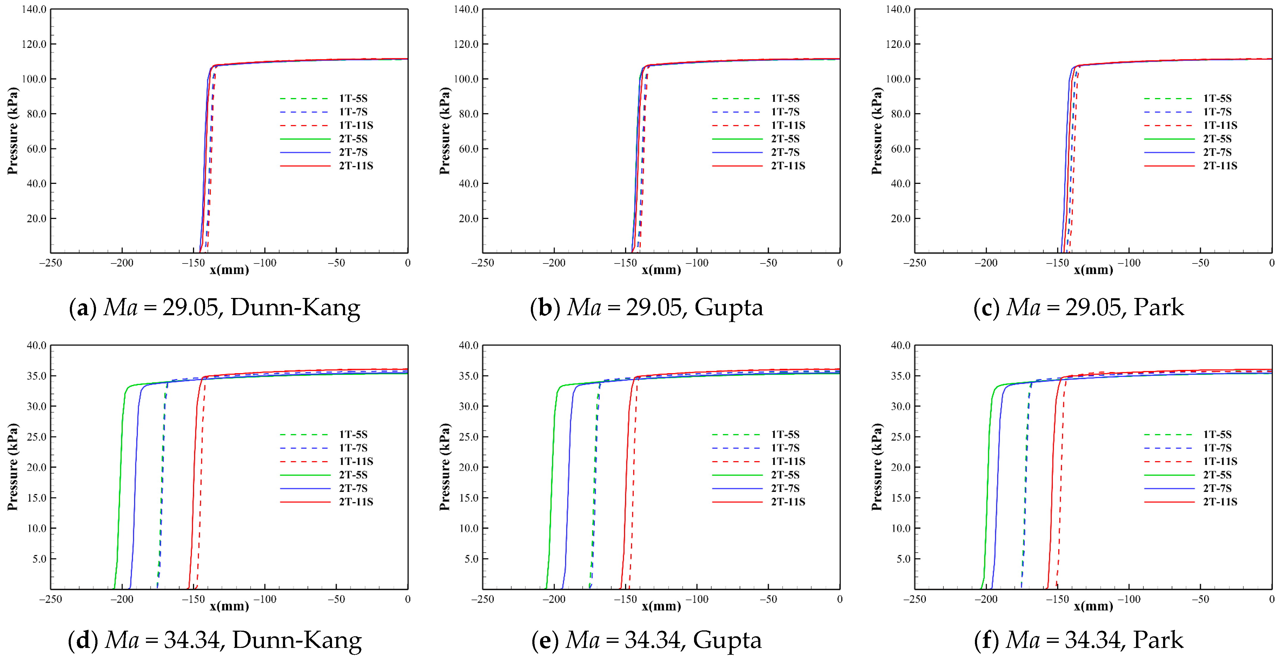
Figure 4 shows the pressure distributions along the stagnation lines computed by the 5-, 7-, and 11-species models of Dunn-Kang, Gupta, and Park combined with the two different temperature models for the three freestream conditions, respectively. It is found that the pressure distributions along the stagnation lines obtained by different models are nearly the same as that of a perfect gas under the same freestream condition. This is because the pressure behind the shock is a “mechanical” parameter that depends mainly on the freestream speed and density. The pressure is uneasily affected by thermochemical nonequilibrium. The pressure behind the shock remains almost constant and its value can be approximated by the relation of pressure ratio across the normal shock.
Figure 2 suggests that the chemical reaction models with different numbers of gas species not only have a significant effect on the shock standoff distance but also the temperature distribution behind the shock. The different numbers of species determine the composition of the gas in the flow field and the number of chemical processes.
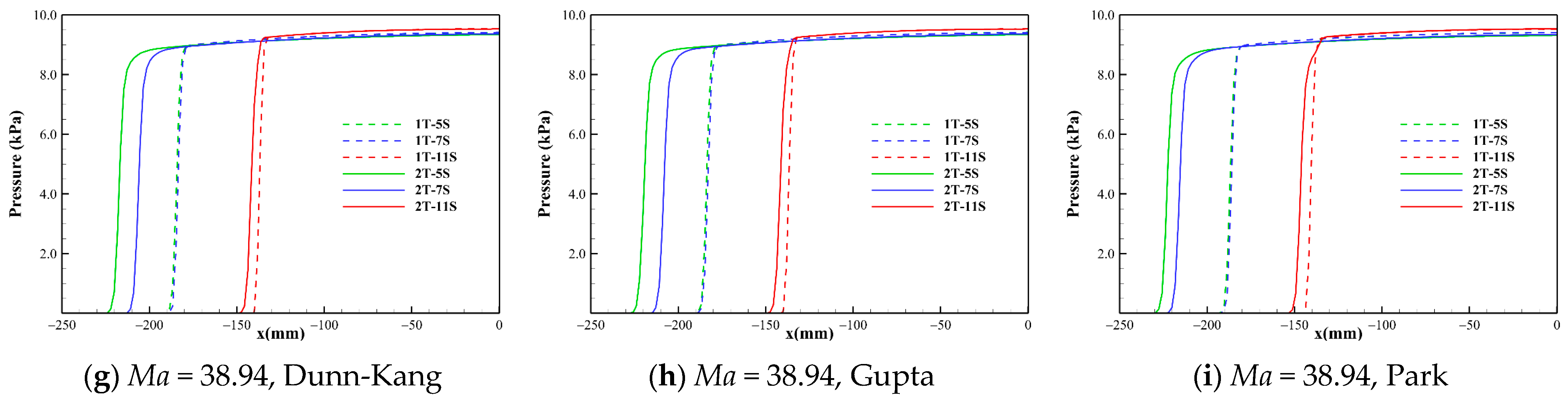
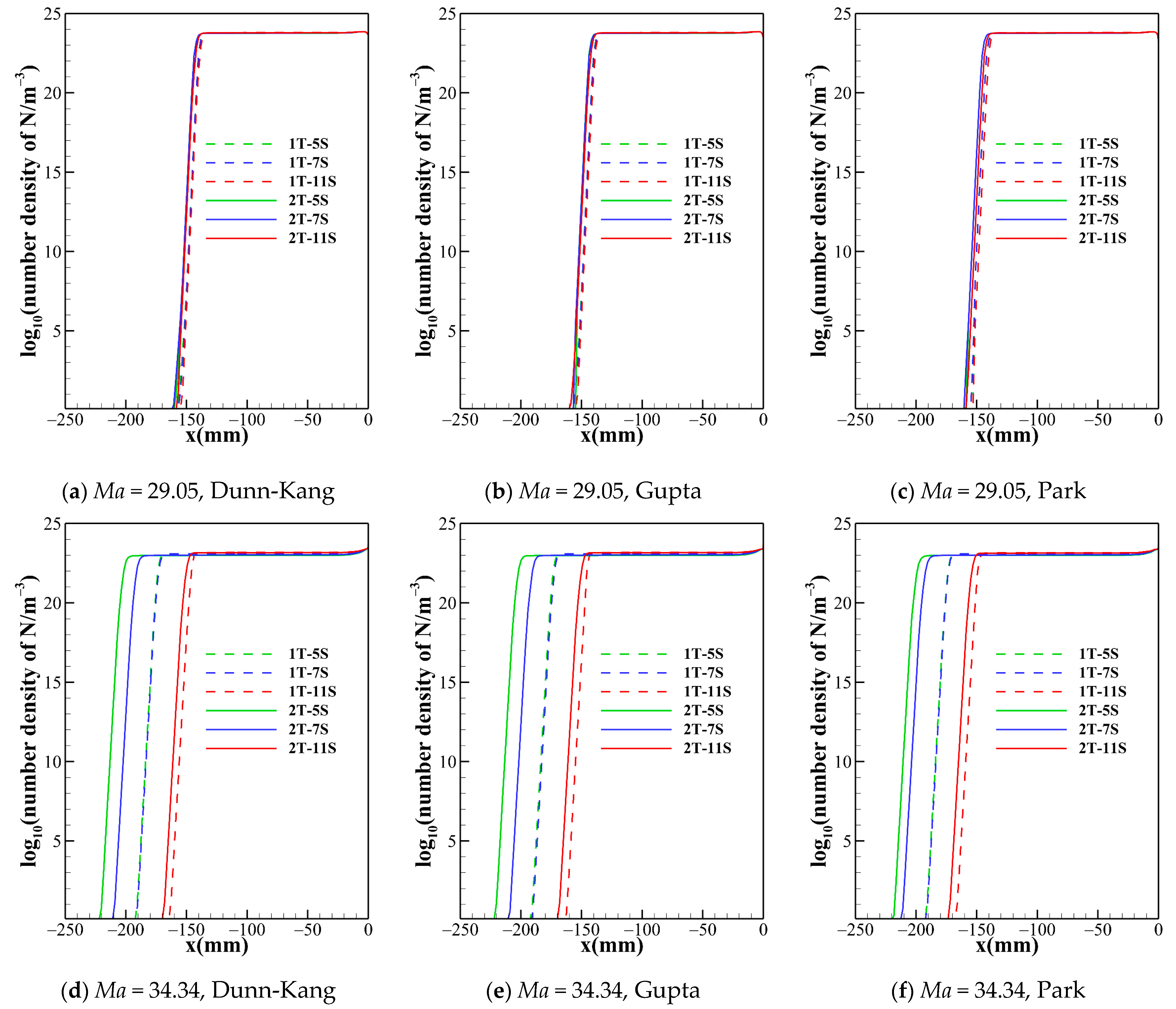
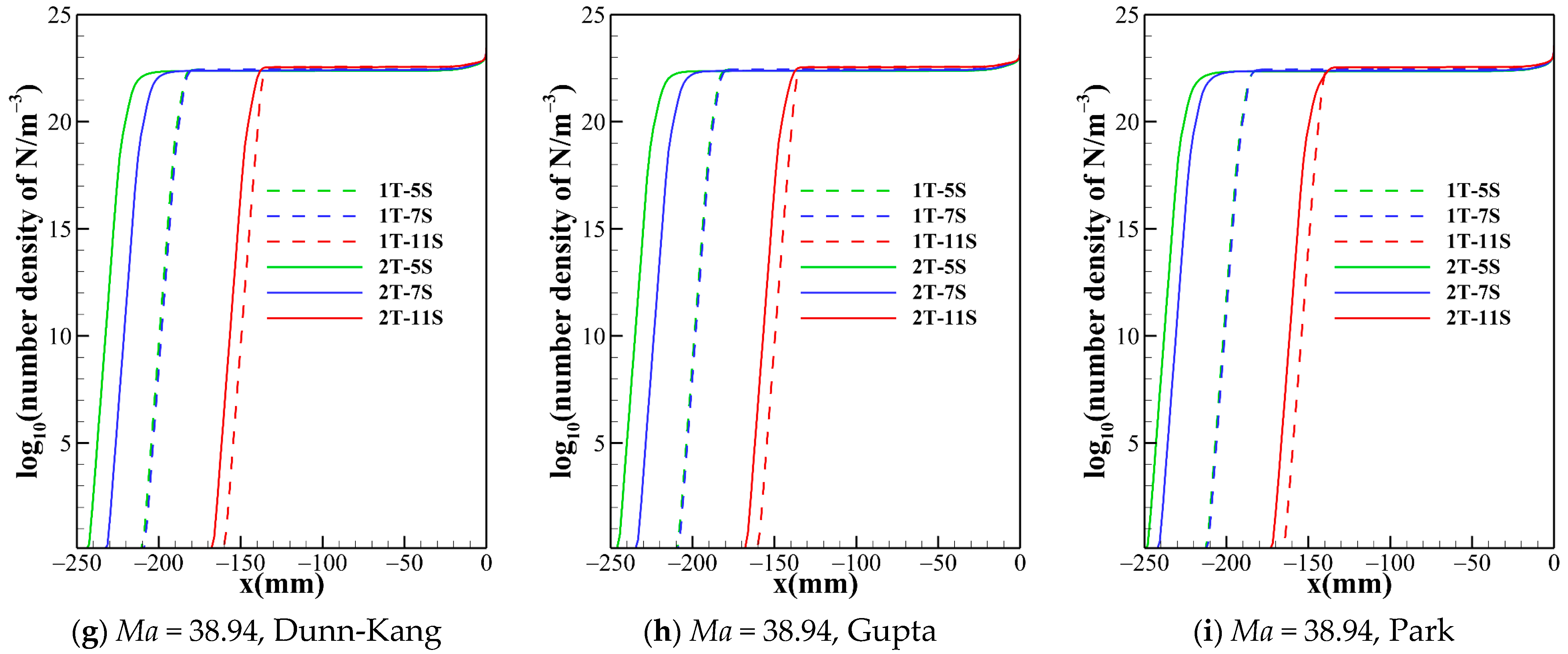
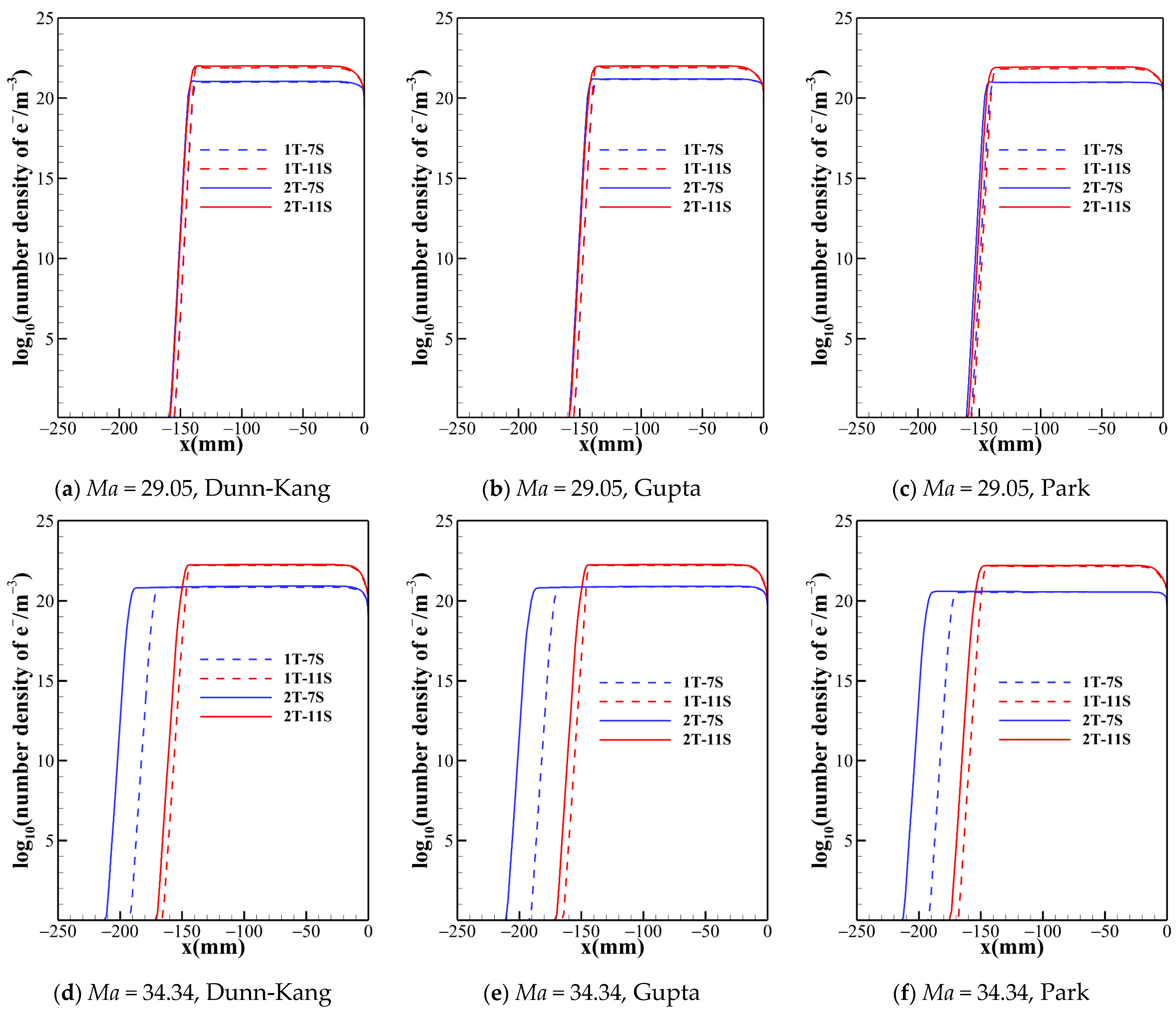
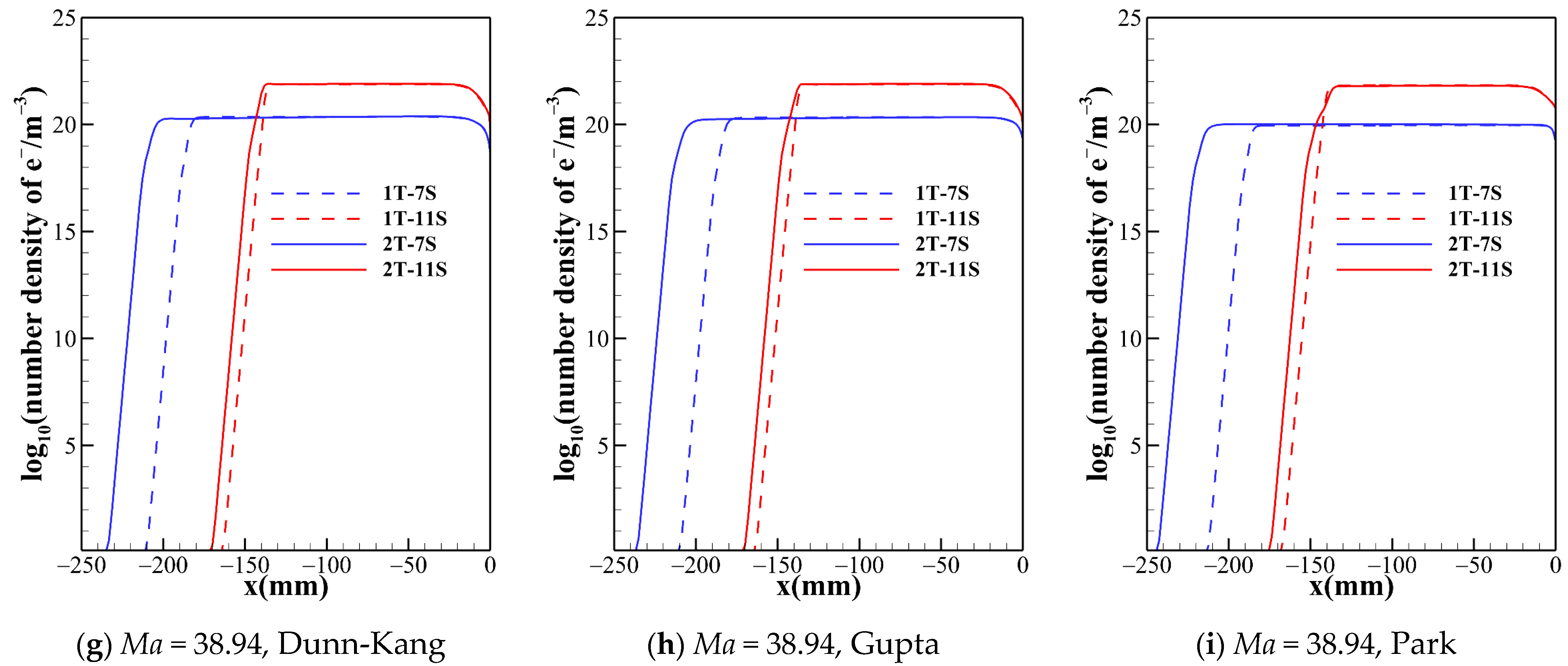
Figure 5 and
Figure 6 show the trend of species number density along the stagnation line predicted by different gas species models. The species number density mainly changes dramatically just behind the shock and near the wall. The curves of N and e
− show the same patterns for both the one- and two-temperature models. The 5-species model contains no ionization reactions, and the diatomic molecules dissociate completely within a small distance behind the shock, while NO is generated. Both the 7-species model and the 11-species model contain ionization reactions. The electrons in the 7-species model are mainly provided by the ionization of a small portion of NO, while the 11-species model contains more ionization reactions, and thus the electron density in the flow field of the 11-species model is significantly higher than that of the 7-species model. Ionization and dissociation reactions are both endothermic processes. Compared to 5- and 7-species models, the 11-species model contains more endothermic reactions, possibly resulting in most conversion of the internal energy of air into the zero-point energy of the reaction products, thus lowest temperature is achieved in the flow field. Under the three freestream conditions, the descending order of translational-rotational temperature for the three models is 5-species > 7-species > 11-species. For all models, because the pressures are almost the same in the shock layer. Therefore, as the temperature of the shock layer increases, the density decreases. Consequently, the order of the shock standoff distance for the three models is 5-species> 7-species>11-species.
To investigate the differences caused by the chemical models with different number of species in detail. The stable values of mass fractions of all species behind the shock wave along the stagnation lines of two cases (
Ma = 29.05 and
Ma = 38.94) are compared in
Table 4. It can be found that at
Ma = 29.05, the proportions of N and O dominate and the total proportion of other species is very little, which means that the 5-, 7- and 11-species models can lead to the similar effects of chemical reactions on the flow simulation. However, at
Ma = 38.94, the ionization reactions become significant and generate considerable quantities of NO
+, N
+ and O
+. In fact, the ionization reactions are endothermic and can lower the temperature level in the shock layer as shown in
Figure 3. Therefore, compared to the case of
Ma = 29.05, the shock layer temperatures obtained by the 5-, 7- and 11-species models decrease in turn more significantly for the case of
Ma = 38.94. As above-mentioned discussion, the chosen number of species in air reaction models has a more significant impact on the shock stand-off distance as the Mach number and altitude grow higher.
Figure 5 shows that the number densities of nitrogen atom reach almost the same level in the shock layer for all model combinations, so is the case of oxygen atom. Therefore, the thermochemical models have no obvious impact on the results of dissociation reactions of O
2 and N
2. However, this situation is not applicable for all species.
Figure 6 demonstrates that, no matter what chemical reaction models are used, there are significant differences in the electron concentration and the shock standoff distance between the two temperature models, which indicates that thermodynamic processes of high temperature air are no longer reliably governed by a single temperature.
3.3. Wall Heat Flux and Pressure
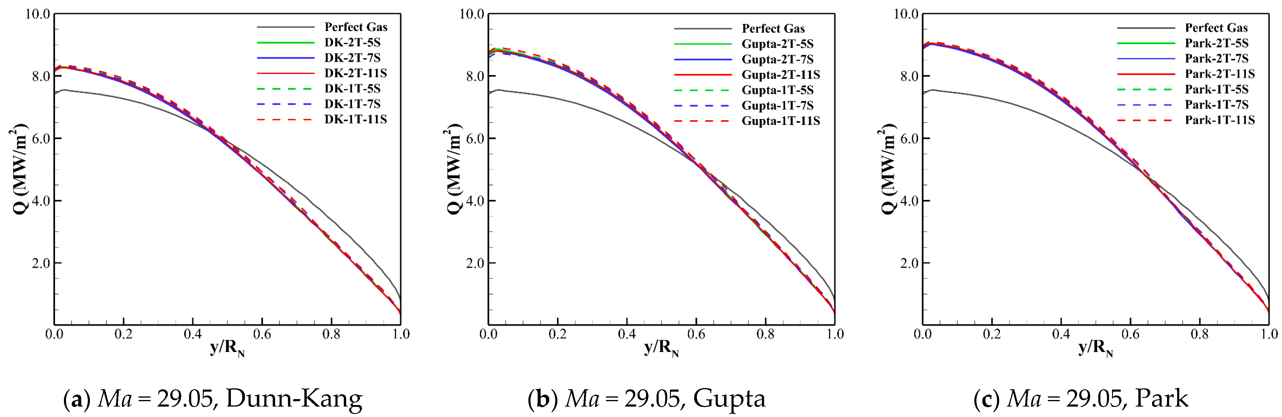
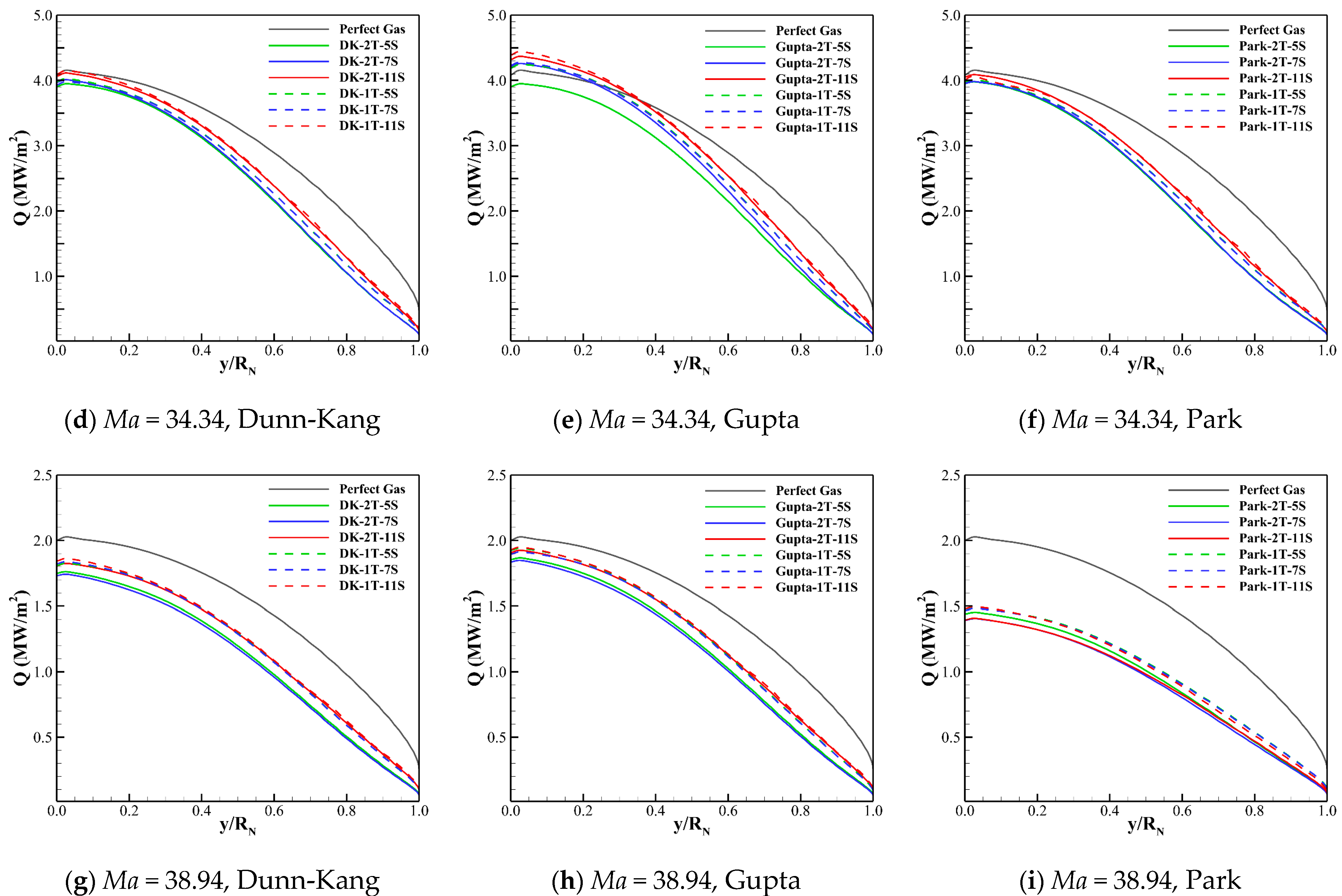
The wall heat fluxes for the three freestream conditions obtained by different thermochemical models and the perfect gas model are compared in
Figure 7. The comparison reveals that there is a significant difference between the wall heat flux of chemical reaction gas and that of perfect gas, and the former can be greater than (
Ma = 29.05), or close to (
Ma = 34.34), or even less than the latter (
Ma = 38.94).
Figure 7 also shows that the differences between the wall heat fluxes predicted by different thermochemical models are small. The wall heat flux of the two-temperature model is always greater than that of the one-temperature model. The Gupta model always gives most conservative results of wall heat transfer compared to the Dunn-Kang and Park models.
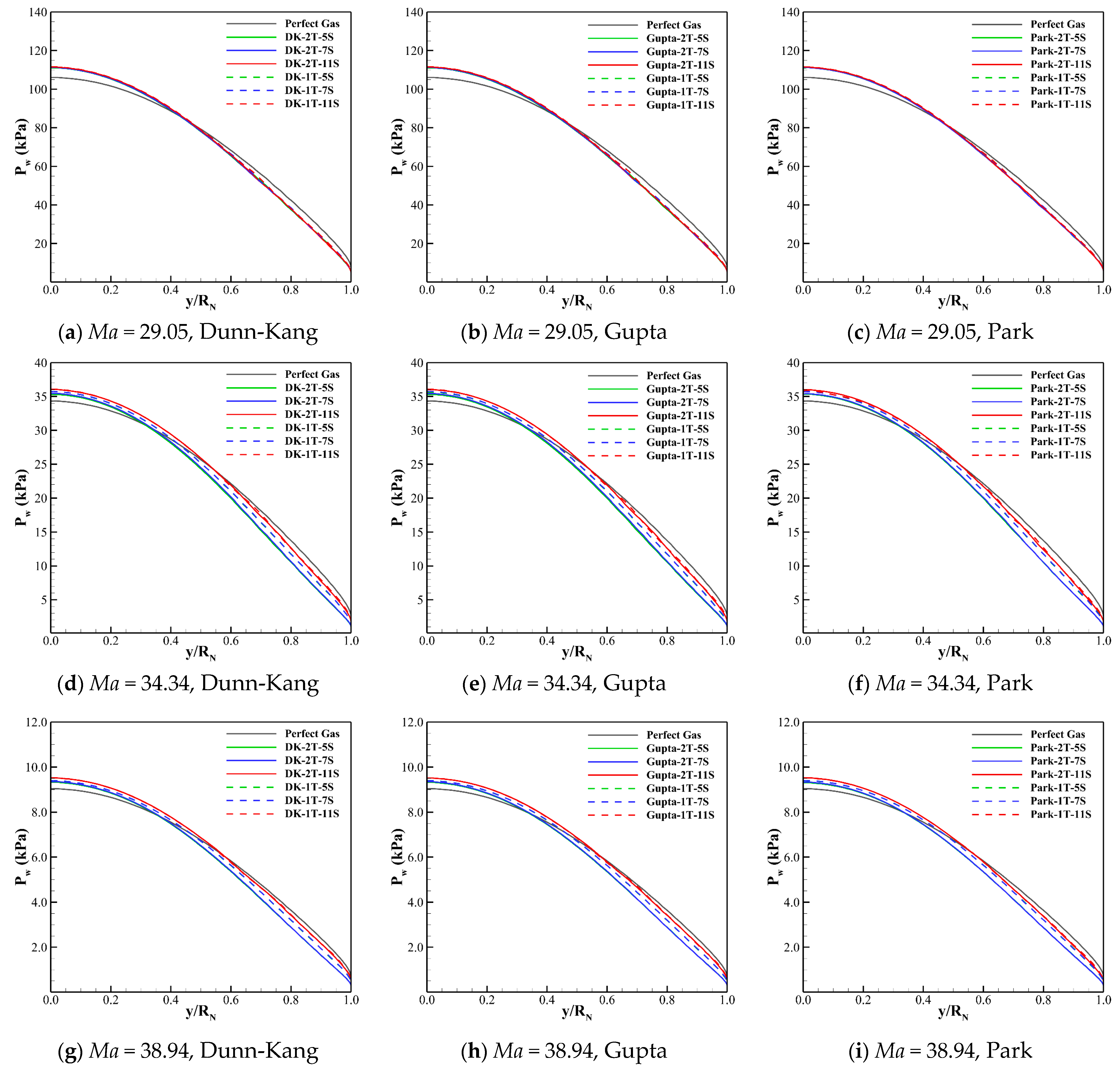
The effects of different models on the wall pressure for the three cases are compared in
Figure 8. Compared to the wall heat transfers, the wall pressures of different thermochemical models are more consistent, including the result of perfect gas. According to
Figure 4 and
Figure 8, it can infer that the different thermochemical models have little influence on the pressure prediction of the hypersonic shock layer. However, such small differences between the wall pressure results of different models still might be amplified by multiplying the displacement in the pitch moment calculation for the hypersonic vehicle, which requires the further investigation using a complex configuration with the angle of attack.
4. Conclusions
There are significant thermochemical processes in the hypersonic and high-temperature flow, for which the perfect gas model is not applicable. Many different models have been proposed to predict the thermodynamic excitations and chemical reactions of high-temperature air. The present study comprehensively investigates the effects of different thermodynamic model combined with different chemical kinetic model on calculating the aerodynamic characteristics using a standard cylinder at extremely high flight speed. Despite the availability of modified reaction kinetic parameters for 11-species [
25], the effect of the reaction kinetic parameters on the flow field will be studied as a future research as HyFLOW currently does not support the modification of reaction kinetic parameters.
At extreme flight conditions, the flow results calculated by the perfect gas model generally deviate greatly from those of thermochemical models. However, at low altitude and low Mach number, the results of pressure and wall heat flux given by the perfect gas model show less deviation compared to those of the thermochemical models. Therefore, the perfect gas model can be used for preliminary prediction.
In theory, the flow results predicted by the 11-species chemical reaction model can be considered to be most accurate compared to those of 5-species and 7-species models. The results of the 5-species and the 7-species models at lower altitude and Mach number are not much different from those of the 11-species model, which can be used for the simplified simulation. However, as the altitude and Mach number rise, the differences between the results of the three models become remarkable, and the accurate flow solution cannot be obtained using the 5-species or 7-species model.
At high altitude and Mach number, it is not suitable to describe the flow field using a one-temperature model, especially when a 5- or 7-species chemical reaction model is simultaneously used. There is a large difference between the results of the shock standoff distance and temperature distribution obtained by the one temperature model and those of the two-temperature model. Meanwhile, the use of different temperature models can affect the process of physicochemical reactions in the flow field with an impact on the species composition. Therefore, at extremely high flight speed, the thermodynamic nonequilibrium effect cannot be neglected and a single mode temperature of internal energy of air cannot be used for a simplified solution.
For the chemical models including the same total number of species, the overall differences between the flow results predicted by the Dunn-Kang, Gupta and Park models are small. The results of the Dunn-Kang model are closer to those of the Gupta model, while the wall heat transfer predicted by the Gupta model is more conservative than those other two models. Therefore, it is proposed to preferentially use the Gupta model for the hypersonic flow simulation in the engineering application.
In summary, if it only focuses on the distribution trends and orders of magnitude of the wall pressure and heat flux, the one-temperature model together with the 5-species model can be used for a quick assessment. However, for the high altitude and extremely high flight speed, the two-temperature model combined with the Gupta 11 species model are recommended to obtain a more reliable solution of the flow field.


