Conversion between Number Systems in Membrane Computing

Abstract

The number system is the representation method of numbers, and number system conversion is the most basic function of a computing system. The decimal system is the most commonly used number system; however, it may not necessarily be the most suitable number system in a computing system. This paper investigates the conversion methods between different number systems and designs corresponding cells, such as P systems, to implement them. The P systems we designed include Π_{10_2} and Π_{2_10} to implement conversion between decimal and binary, Π_{10_m} and Π_{m_10} to implement conversion between decimal and m-base. The operation process of each P system was explained through examples, and their feasibility and effectiveness were verified through simulation software, UPSimulator.

1. Introduction

Membrane computing is a new branch of biocomputing. In 1998, the Romanian scientist Gheorghe Păun developed the idea of membrane computing based on the study of the life processes of cell membranes in living organisms by proposing and studying some of the characteristics of membranes and some of the properties of computing [1]. The membrane computational model abstracts each biological cell into a region surrounded by membranes. In this way, each biological cell is abstracted into multiple regions with a hierarchical structure, each region being called a membrane; i.e., regions correspond to membranes one by one. Each region contains a multiset of objects that evolve according to the evolutionary rules of the region in which they are located, and the evolutionary rules vary from region to region. Thus, each membrane can be considered a separate computational unit to perform the corresponding calculation. Because of the incredible number of cells in an organism and the small amount of energy required for biochemical reactions, one of the greatest advantages of membrane computing is that it enables the corresponding calculations to be carried out in maximal parallel. It has been shown in the literature [1] that membrane computing is equivalent to Turing machines and that its powerful parallel computing capabilities can effectively solve the computational bottlenecks faced by current electronic computers.

The basic idea of membrane computing is to transform computational problems into biological processes in membrane systems, solving problems through reactions within the membrane system. There are currently three main types of membrane systems: cell-like P systems [2], tissue-like P systems [3], and neural-like P systems [4]. In this paper, we discuss the cell-like P system, which mainly includes the transfer P system, the transit P system, and the active membrane P system. The transfer p system is the first introduced and most basic model of membrane computation, which mainly uses multiple set rewriting and communication rules to accomplish the computation, where the computation is mainly within the membrane structure. In order to achieve a flow of objects between membranes, such as the result of computation within one membrane structure as the initial object of a rule execution within another membrane structure, a mechanism is needed that allows the flow of substances between membrane structures, and thus the transit P system is proposed [5]. The active membrane P system [6,7,8] can treat not only elements in multiple sets but also membranes. It can dissolve, generate, split, and merge membranes. When the membrane is dissolved, the objects inside the membrane will be released into the outer membrane, and the rules inside the membrane will not exist. When membranes merge, the objects and rules in each of the merged membranes will exist simultaneously within a single membrane structure.

Numerical computation as a field of membrane computing research and application has yielded some results: Reference [9] designed four basic arithmetic operators based on neural P systems for addition, subtraction, multiplication, and division, achieving basic arithmetic operations. Reference [10] designs the implementation of the corresponding spiking neural P systems, including two’s complement, addition /subtraction on signed integers, and multiplication on two arbitrary natural numbers. In reference [11], the author proposed a complete arithmetic calculator implemented by spiking neural P systems and also gave its application in information fusion. Reference [12] implements arithmetic operations for cell-like P systems with multilayer cell membranes. Reference [13] further improves on reference [12] by using a single membrane structure to achieve arithmetic operations. A new arithmetic P system is proposed in reference [14], which can perform four basic operations. By directly placing the digits of decimal integers into the layered membrane, the number of membranes is reduced, thereby reducing complexity. In [15], multimembrane P systems are constructed for signed arithmetic operations. Reference [16] implements an arithmetic operation on a rational number field, and reference [17] introduces the method of unsigned fraction reduction. In addition, in order to simulate hybrid P systems, a simulator called UPSimulator was proposed in reference [18], which can serve as a development library for P system models. This model processes objects in the region defined by membranes and supports complex evolutionary rules and structures in different types of P systems. This simulator serves as the main tool for verifying the correctness of the membrane rules in Section 5.

Modern computers are still based on von Neumann’s architecture, a feature of which is that data and instructions are represented in binary form. The reasons for using binary are as follows: (1) Binary only needs two states to represent numbers. It is easy to implement binary numbers ‘0’ and ‘1’ using bistable circuits in computers. In order to solve the problem of binary writing length, octal and hexadecimal systems have also been introduced in computers. (2) The rule of binary calculation is simple. Addition is the most basic operation, and multiplication is the continuous addition operation. It is easy to realize subtraction and division based on addition and multiplication by the complement code. (3) Binary operations are easier to implement than logical operations. The binary ‘0’ and ‘1’ exactly correspond to the logical quantities “true” and “false”. (4) The conversion of binary to other decimal systems is easy to implement both in theory and in practice.

From KB-level files to GB-level video software to massive data files, all are stored in binary form on a computer or server. Among them, the conversion between the number systems plays an important role in computers. There are two main reasons: (1) Easier human-computer interaction. The binary used in computers is a 2-based system; however, humans usually use a decimal system. Therefore, performing the base conversion on a computer can help us convert between different bases and represent, process, and transmit numbers. (2) This paper provides an idea for a multidecimal conversion. Decimal is the familiar system; however, it is less clear what number system was used in the P system implemented in later biological computers.

The basis of numerical computation is the representation of values in the computing system, that is, the numerical system. The efficiency of different numerical systems in different computing systems will also vary. For example, the use of binary form in electronic computers can make good use of the performance of electronic presence and computing devices. Quadrature is more appropriate for DNA computing. Spiking neural P systems usually use binary, and cell-like P systems use decimals more. According to the references we have looked at so far, there has been no systematic study of P systems for binary conversion. To further prove the convenience of numerical calculation in membrane computing systems, this paper systematically studies the cell-like conversion P system. This paper mainly discusses the implementation of decimal-to-binary and m-to-decimal conversions. The main contributions of this paper are:

(i)

In this paper, we design a cell-like P system with different base conversions. They include conversions between binary and decimal and conversions between decimal and the base m.

(ii)

The feasibility and validity of the P system for conversion between multiple decimal systems are verified by the simulation software UPSimulator [18].

The remainder of this paper is structured as follows: Section 2 will introduce the research background of this paper, including an introduction to the P system, the definition of the P system, and the general method of conversion. Section 3 introduces the P system for conversion between decimal and binary, the rules of evolution, and the implementation of specific examples. The fourth section generalizes further based on the third section and introduces the P system, the evolution rules, and the realization of concrete examples. Section 5 introduces the implementation of the binary conversion, using the UPSimulator simulation software for the example implementation, and gives a brief introduction to its workflow. Section 6 is a summary of the work in this paper.

2. Research Foundation

2.1. Cell-like P Systems

P system is the embodiment of the concrete model of membrane computing, and it is a kind of computing system. The computational task can be designed by constructing evolutionary rules and initial objects for membrane structures. The structure of the cell-like P system is shown in Figure 1. The external membrane in the P system is called skin, separating the entire membrane system from the external environment. A membrane without any other membrane inside it is said to be an elementary membrane [19].

The basic model of the cell-like P system is defined as Formula (1) [2].

Π = (V, μ, ω₁, …, ω_m, R₁, …, R_m, i_o)

(1)

where:

(i)

V is a finite, non-empty alphabet whose elements are objects.

(ii)

μ is a membrane structure with m membrane, labeled by 1, 2, …, m. Membrane with label i, which we call membrane i.

(iii)

ω_i (1 ≤ i ≤ m) is string over V representing the multiset of objects placed in membrane i.

(iv)

R_i (1 ≤ i ≤ m) are finite sets of possible evolution rules over V associated with the membrane i. The following three main forms of rules appear in this paper: (1) Rewriting rule u→v. Consuming a multiset of objects u generates a multiset of objects v. (2) Multiset of objects in or out of the membrane (v, in_i) (v, out). (v, in_i) denotes a multiset of objects v leaving the current membrane into its submembrane. (v, out) shows that the multiset of objects v leaves the current membrane and enters its outer membrane. (3) A multiset of objects disappears u→λ and v→δ. u→λ indicates that in the current membrane, the multiset of objects u are consumed, and no objects are generated. v→δ represents that the multiset of objects v is consumed and no object is generated, while the membrane in which v is located is dissolved.

(v)

i_o is a number between 1 and m where the output of results in Π.

The execution of rules in Π is characterized by both maximally parallel and nondeterministic behavior [19]. The attractive feature of the P system mentioned in reference [2] is its intrinsic parallelism. All objects having access to a rule should use that rule. Moreover, all membranes work in parallel. Maximally parallel means that all the rules that satisfy the conditions in the evolutionary rules at any time will be executed at the same time to improve the efficiency of the system. Nondeterministic means that when there are multiple rules whose execution conditions can be satisfied but only some of them can be satisfied at the same time, the system randomly selects some of the rules to be implemented and objects in the system to evolve, and the rules governing this evolution are chosen in a nondeterministic way [19].

In this paper, we introduce a time slice to measure the efficiency of the P system. We assume that each rule takes the same amount of time to execute. The time taken for each execution of all rules that meet the conditions is a one-time slice. All rules that meet the conditions will be executed in parallel within each time slice.

2.2. Number System Conversion Method

There are three concepts in the number system conversion: number system, cardinality, and bit weight. The number system, also known as the counting system, is a method of representing numerical values with a fixed set of symbols and uniform rules [20]. Cardinality is the number of different numeric symbols that can be used on each digit. For example, binary uses 0 and 1, with a cardinality of 2. Bit weight indicates the weight of the digit at different positions [21], i.e., the value of ‘1’ in a certain place in the number system. For example, in binary, the 2nd-bit weight is 2, and the 2nd-bit weight is 4.

The main methods used for conversion are the Positional expansion method and the Quotient division method.

The positional expansion method is that we multiply the number on each bit with its corresponding bit weight and sum all the products. We assume that the conversion from r decimal to decimal. Then the desired decimal number is:

A₁ + A₂*r + A₃*r² + A₄*r³… + A_n*rⁿ⁻¹

A₁, A₂, A₃, A₄, …, A_n represents the number on each bit of the r decimal number, and 0 ≤ A_i ≤ r − 1, 1 ≤ i ≤ n

The quotient division method is: For example, if we convert from decimal A to r decimal, we divide by r one at a time and take the remainder in reverse order. Then the process is as follows.

(1)

Divide A by r to obtain the quotient and remainder.

(2)

Divide the quotient obtained by dividing in the previous step by r to obtain the new quotient and remainder.

(3)

Repeat (2) until the quotient is 0. The resulting remainder is arranged in reverse order to obtain the resulting binary number.

In this paper, n-bit binary and n-bit m-binary are converted to decimals using the bitwise expansion method. The conversion of decimals to binary and m decimals is carried out by the division and remainder method.

3. Conversion between Decimal and Binary

In this section, we will discuss the membrane structure and evolution rules of decimal-to-binary and binary-to-decimal conversion, respectively.

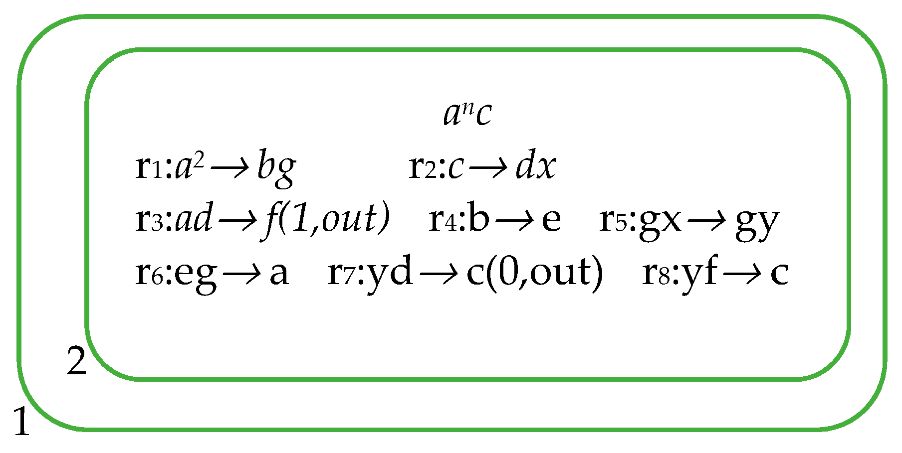
3.1. Decimal to Binary

In order to implement the decimal-to-binary conversion, design the P system structure as (2).

Π_{10_2} = (V, μ, ω₁, R, i_o)

(2)

where

• V = {a, b, c, d, g, x, y, e, g, f}
• μ = [₁[2]₂]₁
• ω₁ = {aⁿc}
• i_o = 1
• R = R₁∪R₂∪R₃
• R₁ = {r₁:a²→bg, r₂:c→dx}
• R₂ = {r₃:ad→ f(1, out), r₄:b→e, r₅:gx→gy}
• R₃ = {r₆:eg→a, r₇:yd→c(0, out), r₈:yf→c}

a, b, c, d, e, g, x, y, and f are objects in the system. n is the number of decimal digits converted to binary. Membrane 1 is where the output results are stored. To visualize this specific P system used to convert decimal to binary, Figure 2 shows its architecture.

Π_{10_2} converts the decimal number n to a binary string. Initially, n objects a (multisets {aⁿ}) and one object c are placed in membrane 2. Rule set R of Π_{10_2} is divided into three subsets_.

R = R₁∪R₂∪R₃

(3)

where

R₁ = {r₁, r₂},⋯R₂ = {r₃, r₄, r₅}, R₃ = {r₆, r₇, r₈}

R₁, R₂, and R₃ correspond to the rules executed in each of the 3 time slices of Π_{10_2} the execution. Every three time slice Π_{10_2} completes a loop to achieve the number of objects a in membrane 1 divided by 2 and outputs a 1-bit binary number to the environment (the order of output is from low to high) until the number of objects a in membrane 2 is zero.

When we convert the decimal number n (represented as aⁿ in membrane 2) to binary, the execution process of Π_{10_2} is as follows:

(1) The first time slice. The rules in R₁ are executed simultaneously; however, one of the special cases is that when |a| < 2 (the quantity of object a is denoted as |a|), only r₂ meets the execution conditions. When r₁ is executed, the number of objects a in membrane 1 is divided by 2 and produces |a|/2 objects b and g (the number of objects b and g represents the quotient of decimal number n divided by radix 2). If n is an odd number, there will be 1 object a left in membrane 1 (the number of a represents the remainder after r₁ is applied). When r₂ is executed, consuming object c generates objects d and x.

(2) The second time slice. The rules in R₂ will be selected for execution. If there is object a in membrane 2, r₃, r₄, and r₅ will be applied; otherwise, only r₄ and r₅ will be executed. The rule r₃ generates objects f and outputs a 1-bit binary number ‘1’ to the environment. Rule r₄ executes, converting |a|/2 objects b to |a|/2 objects e. Rule r₅ executes, converting objects x and g to objects y and g. After the second time slice, the number of g remains unchanged, which is still |a|/2.

(3) The third time slice. The rules in R₃ will also be selected for execution. If there is object d in membrane 2, r₆ and r₇ are applied, or r₆ and r₈ will be executed. Rule r₆ consumes and converts |a|/2 objects e and g into |a|/2 objects a in preparation for the next cycle. When r₇ is executed, it consumes objects y and d to produce object c and outputs a 1-bit binary number ‘0’ to the environment. Rule r₈ executes, consuming objects y and f to produce object c. Object c is generated to prepare for the next cycle.

After the execution of three time slices is completed, the original n becomes n/2. n/2 will be used as the number of a that will execute the first time slice in the next round, that is, n. The input for the next round of execution will become a^n/2c. The system will always execute the rules in 3-time slices. In Π_{10_2}, n will continue to become half of the original through r₁, and output ‘0’ or ‘1’ through r₃ or r₇ until the system’s rule execution conditions are not met.

From the above, it can be seen that for each loop executed in Π_{10_2} (which requires 3 time slices), the number of a will be reduced by half until |a| = 0, while generating the corresponding binary string. This indicates that Π_{10_2} can correctly complete the conversion from a decimal number to a binary number.

By analyzing Π_{10_2}, we know that each cycle will generate a 1-bit binary number and take 3-time slices. The total time slices taken by Π_{10_2} are related to the converted binary digits. If the number of bits of decimal number n converted by the system is m bits, the total time spent by the system is 3(m − 1) + 2.

To further illustrate the execution of Π_{10_2}, we list the regular execution process and the changes in the number of objects in the membrane in

Table 1. The process of converting a decimal number ‘10’ to a binary number ‘1010′.

Number of Cycles	Time Slice	Multiset of Objects	Implemented Rules	Results	Output in the Environment
1	1	a10,c	r1,r2	b5 g5 d x
1	2	b5 g5 d x	r4,r5	e5 g5 d y
1	3	e5 g5 d y	r6,r7	a5 c	0
2	4	a5 c	r1,r2	b2 a g2 d x
2	5	b2 a g2 d x	r3,r4,r5	f e2 g2 y	1
2	6	f e2 g2 d x	r6,r8	a2 c
3	7	a2 c	r1,r2	b g d x
3	8	b g d x	r4,r5	e d g y
3	9	e d g y	r6,r7	a c	0
4	10	a c	r2	a d x
4	11	a d x	r3	f x	1

, using the decimal number n = 10 as an example.

The conversion of the decimal number ‘10’ to ‘1010′ takes 11-time slices and 4 loops. The loop generates a binary number one bit at a time. 0, 1, 0, and 1 are generated at the 3rd, 5th, 9th, and 11th time slice, respectively. After the rules of the 11th time slice are executed, no more rules are satisfied in the system, the loop terminates, and the system enters the stop state.

3.2. Binary to Decimal

The P system to implement binary-to-decimal conversion up to n bits can be constructed as (4):

Π_{2_10} = (V, μ, ω₁, R, i_o)

(4)

where:

• V = {a, b, c, d, e, p, q, r, x, y, z, λ}
• μ = [1]₁
• ω₁ = {a}
• i_o = 1
• R = R₁∪R₂∪R₃∪R₄
• R₁ = {r₁:0a→ber, r₂:1a→ber}
• R₂ = {r₃:0b→px^{2^(n−1)}c^{2^(n−1)}, r₄:1b→px^{2^(n−1)}d^{2^(n−1)}}
• R₃ = {r₅:ce→cz², r₆:de→dz²r², r₇:x→y, r₈:p→q}
• R₄ = {r₉:z→e, r_10:cy→λ, r₁₁:dy→λ, r₁₂:q→b}

a, b, c, d, e, p, q, r, x, y, z, and λ are objects in the system. n represents the maximum number of bits that can be converted, meaning that the P system can convert binary strings that do not exceed n bits. To visualize this specific P system used to convert binary to decimal, Figure 3 shows its architecture.

Π_{2_10} is used to convert binary numbers with no more than n digits into decimal numbers. Initially, a object is placed in membrane 1. Rule set R of Π_{2_10} is divided into four subsets.

R = R₁∪R₂∪R₃∪R₄

(5)

where:

R₁ = {r₁, r₂}, R₂ = {r₃, r₄}, R₃ = {r₅, r₆, r_7, r₈}, R₄ = {r₉, r₁₀, r₁₁, r₁₂}

Π_{2_10} receives binary strings from the environment from low to high, each bit input is ‘ 0’ or ‘ 1’. The rule in R₁ implements the conversion of the first bit of the input binary, which takes 1 time slice. Starting from the second bit of the input binary number, the rules in R₂, R₃, and R₄ are executed in turn every 3-time slices to complete the conversion of a binary number to a decimal number. When each bit of the binary number is converted, the final number of object r in membrane 1 is expressed as the converted decimal number.

We assume that the binary string is A_mA_m−1…A₁, and the initial decimal number |r| = 0. A_mA_m−1…A₁ in Π_{2_10} is converted to a decimal number as follows:

(1) The system executes the first bit, A₁. The rules in R₁ will be selected for execution. After the rules in R₁ are executed, the current decimal number |r| is equal to the original number |r| plus the number of objects r. If A₁ is ‘0′, then r₁ is applied and produces objects b and e, keeping |r| = 0 unchanged. If A₁ is ‘1’, r₂ is applied and produces objects b, e, and r, making |r| = 1.

(2) The system executes other bits A_s (1 < s ≤ m), including the following two cases:

Case 1: A_s is ‘0’ The rules in R are executed as follows:

① Rule r₃ in R₂ executes the consumption object b to generate object p, 2ⁿ⁻¹ objects x, and object c.

② Rules r₅, r₇ and r₈ in R₄ will be in parallel. Rule r₅ executes consuming objects c and e to generate object c and twice the number of object z. When executed to the A_s, there are 2^s−2 objects e in the system; it produces 2^s−1 objects z after r₅ is applied, keeping |r| unchanged. Rule r₇ executes the consumption object x to generate the object y. Rule r₈ executes, consuming object p to generate object q.

③ Rules r₉, r_10, and r₁₂ are applied in this step. Rule r₁₀ executes, consuming all objects d and y without generating new ones. Rule r₉ executes, consuming all objects z and converting them into the same number of objects e, representing the weight of the current bit. According to the results in ②, there are 2^s−1 objects e in the system after r₉ is applied. Rule r₁₂ consumes object q to generate object b in preparation for converting the next binary input.

Case 2: A_s is ‘1’ The rules in R are executed as follows:

① Rule r₄ in R₂ executes the consumption object b to generate object p, 2ⁿ⁻¹ objects x and object d.

② Rule r₆, r₇ and r₈ in R₃ are applied. Rule r₆ performs the process of consuming objects d and e to generate object d and double the number of objects z and r. When executed to the A_s, there are 2^s−2 objects e in Π_{2_10}. So after r₆ is applied, there are 2^s−1 objects z and r in the system, where |r| = |r| + 2^s−1. Rule r₇ executes the consumption object x to generate the object y. Rule r₈ executes, consuming object p to generate object q.

③ Rules r₉, r_11, and r₁₂ in R₄ will execute at the same time. Rule r₁₁ causes the system to eliminate objects d and y when the next binary bit executes the first step. Rules r₉ and r₁₁. The execution process of rules r₉ and r₁₂ is the same as that of r₉ and r₁₂ mentioned in the ③ of Case 1, and it will not be repeated here

The result after completing step ③ in Case 1 or Case 2 is be^s−1 and be^s−1 will be used as the initial input when the next binary bit performs an operation in Π_{2_10}.

In summary, after the input of the binary string A_mA_m−1…A₁ ends, the number of objects r in the system is A₁ + A₂ * 2 + … + A_m * 2^m−1. Therefore, Π_{2_10} can correctly realize the conversion from a binary number to a decimal number.

From the analysis of the rule set of Π_{2_10} and its execution process, it is clear that it takes 3(n − 1) + 1 time slice to convert n-bit binary numbers to decimal numbers. The n here represents the actual number of bits in the binary string.

To further illustrate the Π_{2_10} execution process, we use the rule set for converting 8-bit binary numbers to decimal numbers to convert binary ‘11010’ to decimal numbers as an example and list the rule execution process and the change in the number of objects in

Table 2. The process of converting the binary number ‘11010’ to the decimal number ’26’.

Number of Cycles	Time Slice	Multiset of Objects before Rule Execution	Implemented Rules	Multiset of Objects after Rule Execution
1	1	a 0	r1	b e
2	2	b e 1	r4	p x128 d128 e
2	3	p x128 d128 e	r6,r7,r8	d128 y128 z2 q r2
2	4	d128 y128 z2 q r2	r1,r2	b e2 r2
3	5	b e2 r2 0	data 1	c128 x128 e2 p r2
3	6	c128 x128 e2 p r2	data 1	c128 y128 z4 q r2
3	7	c128 y128 z4 q r2	r9,r10,	e4 b r2
4	8	e4 b r2 1	r4	d128 x128 e4 p r2
4	9	d128 x128 e4 p r2	r6,r7,r8	d128 y128 z8 q r10
4	10	d128 y128 z8 q r10	r9,r11,r12	b e8 r10
5	11	b e8 r10 1	r4	d128 x128 e8 p r10
5	12	d128 x128 e8 p r10	r6,r7,r8	d128 y128 z16 q r26
5	13	d128 y128 z16 q r26	r9,r11,r12	b e16 r26

. It should be noted that the 8-bit binary conversion rules for r₃ and r₄ are specifically expressed as r₃: 0b→px¹²⁸c¹²⁸, r₄: 1b→px¹²⁸d¹²⁸. The rest of the rules remain the same.

The conversion of the binary number ’11010’ to the decimal number ‘26’ takes 13-time slices and 5 loops. With no more new binary bits entering the system, the system’s calculations stop, and the number of r in the final membrane 1 represents the value of the converted decimal number, which is 26.

4. Conversion between Decimal and m-Binary

Based on Section 3, this section further expands the discussion of the membrane structure and evolutionary rules for decimal to m-binary and n-bit m-binary to decimal.

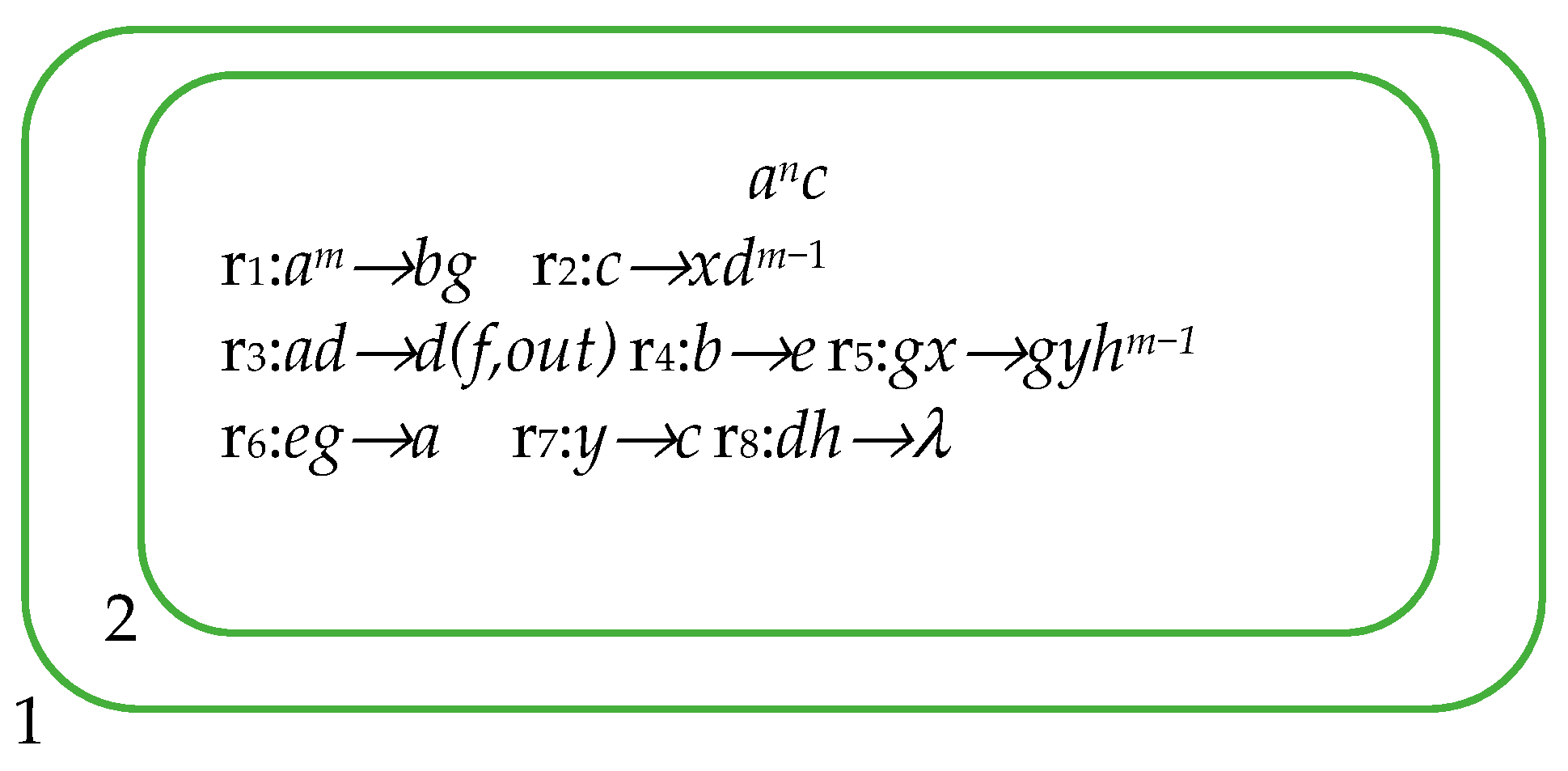
4.1. Decimal to m-Binary

The P system for decimal to m-binary is as (6).

Π_{10_m} = (V, μ, ω₁, R, i_o)

(6)

where:

• V = {a, b, c, d, e, f, g, h, λ}
• μ = [₁[2]₂]₁
• ω₁ = {aⁿc}
• i_o = 1
• R = R₁∪R₂∪R₃
• R₁ = {r₁:a^m→bg, r₂:c→xd^m−1}
• R₂ = {r₃:ad→d(f,out), r₄:b→e, r₅:gx→gyh^m−1}
• R₃ = {r₆:eg→a, r₇:y→c, r₈:dh→λ}

a, b, c, d, e, f, g, h, and λ are objects in the system. n is the number of decimal digits converted to binary. membrane 0 is the environment. To visualize this specific P system used to convert decimal to m-binary, Figure 4 shows its architecture.

Π_{10_m} converts decimal numbers to m. Initially, membrane 1 contains n objects a (multisets {aⁿ}, representing the decimal number n to be converted) and 1 object c. The rule for Π_{10_m} is divided into three subsets:

R = R₁∪R₂∪R₃

(7)

where:

R₁ = {r₁, r₂}, R₂ = {r₃, r₄, r₅}, R₃ = {r₆, r₇, r₈}

They correspond to 3-time slices of Π_{10_m}. Each 3 time slices, the P system completes a loop that divides the number of objects a in membrane 1 by m and outputs a 1-digit m decimal number to the environment |f| (|f| represents the number of objects f), until the number of objects a is zero. In the environment, you will receive the conversion result in turn from the lowest bit to the highest bit of each digit value (m decimal).

We suppose that the decimal number to be converted is n and the i-th bit of the converted binary number is A_i. Then the converted m-binary string is A_sA_s−1…A₁ (s ≥ 1). The following (1), (2), and (3) describe the process of generating A_i (1 ≤ i ≤ s).

(1) In the first time slice. The rules in R₁ are executed concurrently; however, only r₂ will be executed if |a| < m (The number of objects a is denoted as |a|). Rule r₁ is executed and produces |a|/m objects b and g. The number of objects b and g generated is the quotient (|a|/m) after r₁. When n is not a multiple of m, there will be |a| % m objects a objects left in membrane 1. Rule r₂ consumes 1 object c to generate 1 object x and m − 1 objects d.

(2) In the second time slice. Some rules in R₂ are applied. When there is a remaining a in membrane 2 (At this time, there are |a|% m objects a in membrane 2), r₃ executes and generate |a| % m objects d and output |a|% m objects f to the environment. The system outputs the remainder through r₃. A_i is equal to the number of objects f. That is, A_i = |a| % m. Rule r₄ executes and convert |a|/m objects b to |a|/m objects e, saving the quotient. When r₅ is applied, it consume object x and g and produce object y, g and m − 1 objects h.

(3) The third time slice. A part of the rules in R₃ can be applied. After step (2), (3) will selectively execute r₆,r₇, and r₈ according to the existing objects in the system. Rule r₆ executes to consume and convert all object e and g to the same number of object a (the number is |a|/m) in preparation for the next round. Rule r₇ is applied and produce object c. Rule r₈ executes to eliminate all object d and h in Π_{10_m}.

Step (1) calculates the remainder and quotient. Step (2) output a 1-bit m-base number A_i, and step (3) prepares for the next digit. After the completion of the three steps, the initial n becomes n/m, and the system will repeat through the above three steps until there are no executable rules in the system. Each time the A_i in Π_{10_m} obtained is arranged from right to left according to the size of the corner markers, forming the final result A_sA_s−1…A_1.

Based on the above description, it can be seen that for each loop executed in Π_{10_m} (which requires 3 time slices), the number of a will be reduced until |a| = 0, while generating the corresponding binary string, meanwhile generating the corresponding binary string. This indicates that Π_{10_m} can correctly complete the conversion from decimal number to m-binary number.

From the rule set of Π_{10_m}, it is known that converting the decimal number n to m decimal requires cycling $[{\log }_{\mathrm{m}}\mathrm{n}]+1$ times for a total of $3\left([{\log }_{\mathrm{m}}\mathrm{n}]+1\right)$ time slices.

The rules r₁, r₂ and r₅ for decimal to m-binary change depending on the binary number m. For example, when converting decimal numbers to octal numbers, the rules for r₁, r₂ and r₅ are: a⁸→bg, c→xd⁷, gx→gyh⁷ respectively. The rest of the rules remain.

To further illustrate the execution process of Π_{10_m}, we take the conversion of the decimal number n = 20 to an octal number as an example and list the rule execution process and the changes in the number of objects in the membrane in

Table 3. The process of converting a decimal number ‘20’ to an octal number ‘42’.

Number of Cycles	Time Slice	Multiset of Objects before Rule Execution	Implemented Rules	Multiset of Objects after Rule Execution	Multiset of Objects after Rule Execution
1	1	a20,c	r1,r2	b2 g2 a4 d7 x
1	2	b2 a4 d7 g2 x	r3,r4,r5	d7 e2 g2 h7 y	f4
1	3	y e2 g2 d7 h7	r6,r7,r8	a2 c
2	4	a2 c	r2	a2 d7 x
2	5	a2 d7 x	r3	d7 x	f2

.

The conversion of decimal number ‘20’ to octal number ‘24’ takes a total of 5 time slices and 2 loops. Each loop generates one octal number. After executing the rules for the fifth time slice, no more rules are satisfied in the system, the loop terminates, and the system stops. The system sends 4 objects f to the environment on the second time slice in the first cycle, so A₁ = 4. At the second time slice of the second cycle, 2 objects f appeared in the system, A₂ = 2. The final octal number generated is A₂A₁ = ‘24’.

4.2. n-Bit m Decimal to Decimal

To achieve the n-bit m decimal to decimal conversion (where m ≥ 3), the p-system structure is designed as in Equation (8):

Π_{m_10} = (V, μ, ω₁, R, i_o)

(8)

where:

• V = {a, b, c, d, g, x, y, e, g, λ, f, r, p, q, u, z, v}
• μ = [₁[2]₂[3]₃…[_m]_m]₁
• ω₁ = {a}
• i_o = 1
• R₁ = {r₁:0_a→be, r₂:1a→ber,…, r_m:(m − 1)a→ber^m−1}
• R₂ = {r_m+1:0b→px^{m^(n−1)}c^{m^(n−1)} (t,in₂)…(t,in_m−1), r_m+2:1b→px^{m^(n−1)}d^{m^(n−1)} (t,in₂)…(t,in_m−1),
• r_m+3:2b→px^{m^(n−1)}d^{m^(n−1)}(px^{m^(n1)}d^{m^(n1)},in₂), …,
• r_2m:(m − 1)b→px^{m^(n−1)}c^{m^(n−1)}(px^{m^(n−1)}d^{m^(n−1)},in₂)…(px^{m^(n−1)}d^{m^(n−1)},in_m−1),
• r_2m+1:e→v(u,in₂)…(u,in_m−1)}
• R₃ = {r_2m+2:cv→cz^m, r_2m+3:dv→dz^mr^m, r_2m+4:x→y, r_2m+5:p→q}
• R₄ = {r_2m+6:z→e, r_2m+7:cy→λ, r_2m+8:dy→λ, r_2m+9:q→b}
• R₅ = {r_2m+10:du→d(r^m,out), r_2m+11:x→y, r_2m+12: p→t}
• R₆ = {r_2m+13:yd→λ, r_2m+14:t→δ}
• R₇ = {r_2m+15:u→λ}

The specific P system used to convert n-bit m decimal to decimal as Figure 5.

The task of Π_{m_10} is to convert n-bit m decimal numbers to decimal numbers. Initially, 1 object a is placed in membrane 1. The rules of Π_{m_10} are divided into seven subsets:

R = R₁∪R₂∪R₃∪R₄∪R₅∪R₆∪R₇

(9)

where:

R₁ = {r₁, r₂…r_m}, R₂ = {r_m+1…r_2m+1}, R₃ = {r_2m+2…r_2m+5}, R₄ = {r_2m+6…r_2m+9}

R_{5 =} {r_2m+10…r_2m+12}, R₆={r_2m+13, r_2m+14}, R₇={r_2m+15}

Π_{m_10} receives and processes the input from the environment in order from the lowest bit to the highest bit of the m-decimal number. The rules in R₁ are used to process the lowest bit input only, and the rules in R₂~R₇ are used to complete the processing of the other bit inputs.

We assume that the binary string is A_nA_n−1…A₁, and the initial decimal number |r| = 0. A_nA_n−1…A₁ in Π_{m_10} is converted to a decimal number as follows:

(1) Firstly, the system executes the first bit A1, The rules r₁ to r_m in R₁ will be selected for execution. The current decimal number |r| is equal to the original number |r| plus the number of object r after R₁ is applied. If there are f objects r in the system, so |r| = |r| + f. For example, If the A₁ is ‘3’, the rule 3a→ber³ in R₁ is activated to consume the input value ‘3’ and object a to generate 1 object b and e and 3 objects r. Then |r| = |r| + 3 = 3.

(2) Π_{m_10} executes other digits A_s(1 < s ≤ n) in the order of ①, ②, ③. We assume that the value of A_s is equal to h (0 ≤ h ≤ m − 1). According to the different values of A_s, it can be divided into the following situations:

Case 1: When A_s is ‘0’, the rules in R are executed as follows:

① Rule r_m+1 and r_2m+1 in R₂ will be applied. Rule r_m+1 will generate 1 object p and mⁿ⁻¹ objects x and c, meanwhile, 1 object t will enter membrane 2 to membrane m − 1. Rule r_2m+1 consume m^s−2 objects e and produce m^s−2 objects v, m^s−2 objects u enters membrane 2, 3, …, m − 1 at the same time.

② Rules r_2m+2, r_2m+4, r_2m+5 in R₃ and r_2m+14 in R_6, execute in parallel. This operation does not produce object r, so |r| remains unchanged. Rule r_2m+14 eliminates object t, dissolves the membrane, and releases all objects u inside the membrane to membrane 1. Rule r_2m+4 and r_2m+5 convert all objects x and p in the system to the same number of objects y and q respectively.

③ Rules r_2m+6, r_2m+7 and r_2m+9 in R₄ and r_2m+15 in R₇ will be executed in this step. Rule r_{2m+ 6} executes consuming all objects z and converting them into the same number of objects e, representing the weight of the current bit. According to the results in ② there are m^s−1 objects e in the system after r_2m+6 is applied. Rule r_2m+7 eliminate all objects c and y in the system. Rule r_2m+9 consumes object q to generate object b in preparation for converting the next binary input. Rule r_2m+15 eliminates all objects u in Π_{m_10}.

Case 2: When A_s is ‘1’, the execution process is as follows:

① Rules r_m+2 and r_2m+1 in R₂ will be execute. Rule r_m+2 generate 1 object pmⁿ⁻¹ objects x and d in membrane 1, meanwhile generate 1 object and enters membrane 2, 3, …, m − 1. The execution of r_2m+1 is the same as ① in Case 1.

② Rules r_2m+3, r_2m+4 and r_2m+5 in R₃ and r_2m+14 in R₆ are applied. The system will generate m^s−1 objects r; therefore, |r| = |r| + m^s−1 after r_2m+3 executes. Rules r_2m+4, r_2m+5 and r_2m+14 is executed exactly like ② in Case 1.

③ Rules r_2m+6, r_2m+8 and r_2m+9 in R₄ and r_2m+15 in R₇ execute in parallel. Rule r_2m+8 eliminate all objects c and y in the system. The execution of r_2m+6, r_2m+9 and r_2m+15 is specified in ③ of Case 1.

Case 3: When A_s is ‘h’ and 2 ≤ h ≤ m − 1, the execution process is as follows:

① Rules r_h+m+1 and r_2m+1in R₂ are applied in this step. The system will generate 1 object p, mⁿ⁻¹ objects x and d in membrane 1, meanwhile 1 object p,mⁿ⁻¹ objects x and d enters membrane 2, 3, …, h after r_h+m+1 execute. The execution of r_2m+1 is the same as ① in Case 1. Rule r_2m+1 consume m^s−2 objects e and produce m^s−2 objects v, m^s−2 objects u enters membrane 2, 3, …, m − 1 at the same time.

② Rules r_2m+3, r_2m+4 and r_2m+5 in R₃ and r_2m+10, r_2m+11 and r_2m+12 in R₅ will be executed in parallel (only R₅ from membrane 2 to membrane h can be executed). By executing the rules r_2m+1 in R₅ from membrane 2 to membrane h, each will output m ^s−1 objects r to membrane 1. Membrane 2 to membrane h output a total of (h − 1) * m^s−1 objects to membrane 1. Membrane 1 generate m ^s−1 objects r after rule r_2m+3 is applied. At this time, there are h*m ^s−1 objects r in membrane 1. Then |r| = |r| + h*m ^s−1. The execution of r_2m+4 and r_2m+5 is the same as ② in Case 1. Rules r_2m+11 and r_2m+12convert all objects x and p in the system to the same number of objects y and t, respectively.

③ Rules r_2m+6, r_2m+8 and r_2m+9 in R₄ and r_2m+13 and r_2m+14 in R₆ are applied. The execution of r_2m+6, r_2m+8 and r_2m+9 is specified in ③ of Case 2. Rule r_2m+13 eliminate all objects y and d in membrane 2, 3, …, h of Π_{m_10}. Rule r_2m+14 eliminates object and dissolves the membrane.

In summary, after the input of the binary string A_nA_n−1…A₁ ends, the number of objects r in the system is A₁ + A₂ * m + … + A_n * mⁿ⁻¹. Therefore, Π _{m_10} can correctly fulfill the conversion from n-bit m decimal numbers to decimal numbers.

From the definition of Π_{m_10} and the process of rule execution, it is clear that the conversion of an n-bit m-decimal number to a decimal number takes 3(n − 1) + 1 time slice.

The membrane structure in Π_m−10 and the rules in R₂ vary with different values of m (m decimal) and n. For example, when considering a 4-bit trinary conversion to decimal, membrane 1 contains only membrane 2, and the rule sets R₂ = {r₄:0b→px²⁷c²⁷, r₅:1b→px²⁷d²⁷, r₆:2b→px²⁷d²⁷(px²⁷d²⁷,in₂), r₇:e→v(u,in₂)}. When considering the n-bit octal conversion to decimal, Membrane 1 contains six sub-membranes: membrane 2~membrane 7, and the rule sets

R₂ = {r₉:0b→px^{8^(n−1}c^{8^(n−1)}(t,in₂)(t,in₃)(t,in₄)(t,in₅)(t,in₆)(t,in₇),

r₁₀:1b→px^{8^(n−1)}d^{8^(n−1}(t,in₂)(t,in₃)(t,in₄)(t,in₅)(t,in₆)(t,in₇),

r₁₁:2b→px^{8^(n−1)}d^{8^(n−1)}(px^{8^(n−1)}d^{8^(n−1)},in₂),

r₁₂:3b→ px^{8^(n−1)}d^{8^(n−1)}(px^{8^(n−1)}d^{8^(n−1)},in₂) (px^{8^(n−1)}d^{8^(n−1)},in₃),

r₁₃:4b→ px^{8^(n−1)}d^{8^(n−1)}(px^{8^(n−1)}d^{8^(n−1)},in₂) (px^{8^(n−1)}d^{8^(n−1)},in₃) (px^{8^(n−1)}d^{8^(n−1)},in₄),

r₁₄:5b→px^{8^(n−1)}d^{8^(n−1)}(px^{8^(n−1)}d^{8^(n−1)},in₂)(px^{8^(n−1)}d^{8^(n−1)},in₃)(px^{8^(n−1)}d^{8^(n−1)},in₄)(px^{8^(n−1)}d^{8^(n−1)},in₅),

r₁₅:6b→px^{8^(n−1)}d^{8^(n−1)}(px^{8^(n−1)}d^{8^(n−1)},in₂)(px^{8^(n−1)}d^{8^(n−1)},in₃)(px^{8^(n−1)}d^{8^(n−1)},in₄)(px^{8^(n−1)}d^{8^(n−1)},in₅) (px^{8^(n−1)}d^{8^(n−1)},in₆),

r₁₆:7b→px^{8^(n−1)}d^{8^(n−1)}(px^{8^(n−1)}d^{8^(n−1)},in₂)(px^{8^(n−1)}d^{8^(n−1)},in₃)(px^{8^(n−1)}d^{8^(n−1)},in₄)(px^{8^(n−1)}d^{8^(n−1)},in₅) (px^{8^(n−1)}d^{8^(n−1)},in₆)(px^{8^(n−1)}d^{8^(n−1)},in₇),

r₁₇:e→v(u,in₂)(u,in₃)(u,in₄)(u,in₅)(u,in₆)(u,in₇)}

Table 4. The process of converting a 3-decimal number ‘1201’ to a decimal number ‘34’.

Number of Cycles	Time Slice	Input	Executable Rules in Membrane 1	Executable Rules in Membrane 2	Results
					Membrane 1	Membrane 2
1	1	1	r2		b e r
2	2	2	r6,r7		p x27 d27 v r	p x27 d27 u
2	3		r9,r10,r11	r16,r17,r18	d27 y27z3 q r7	d27 y27 t
2	4		r12,r14,r15	r19,r20	b e3 r7
3	5	0	r4,r7		p x27 c27 v3 r	u3 t
3	6		r8,r10,r11	r20	c27 y27 z9 u3 r7
3	7		r12,r13,r15,r21		b e9 r7
4	8	1	r5,r7		p x27 d27 v9 r7	u9 t
4	9		r9,r10,r11	r20	d27 z27 y27 u9 q r34
4	10		r12,r14,r15,r21		b e27 r34

gives the execution of Π_{3_10} when converting the 4-bit trinary number ‘1021’ to a decimal number. The membrane structure of Π_{3_10} is [1[2]₂]₁, and the initial multiset in membrane 1 is {a}. The specific membrane structure and rules are shown in Figure 6.

In Table 4, the number of objects r is the value converted to a decimal number. It is clear that the trinary number ‘1021’ is converted to the decimal number ‘34’ and takes a total of 10 time slices.

5. Simulation and Validation of Rules

This section is based on Section 3 and Section 4 and goes further to verify the correctness of the rules in the P system. Simulation experiments with UPSimulator [18] for the examples mentioned in Section 3 and Section 4. The main discussion is on the conversion of decimal number ‘10’ to binary number ‘1010’ and 4-bit 3-decimal number ‘1021’ to decimal number ‘34’.

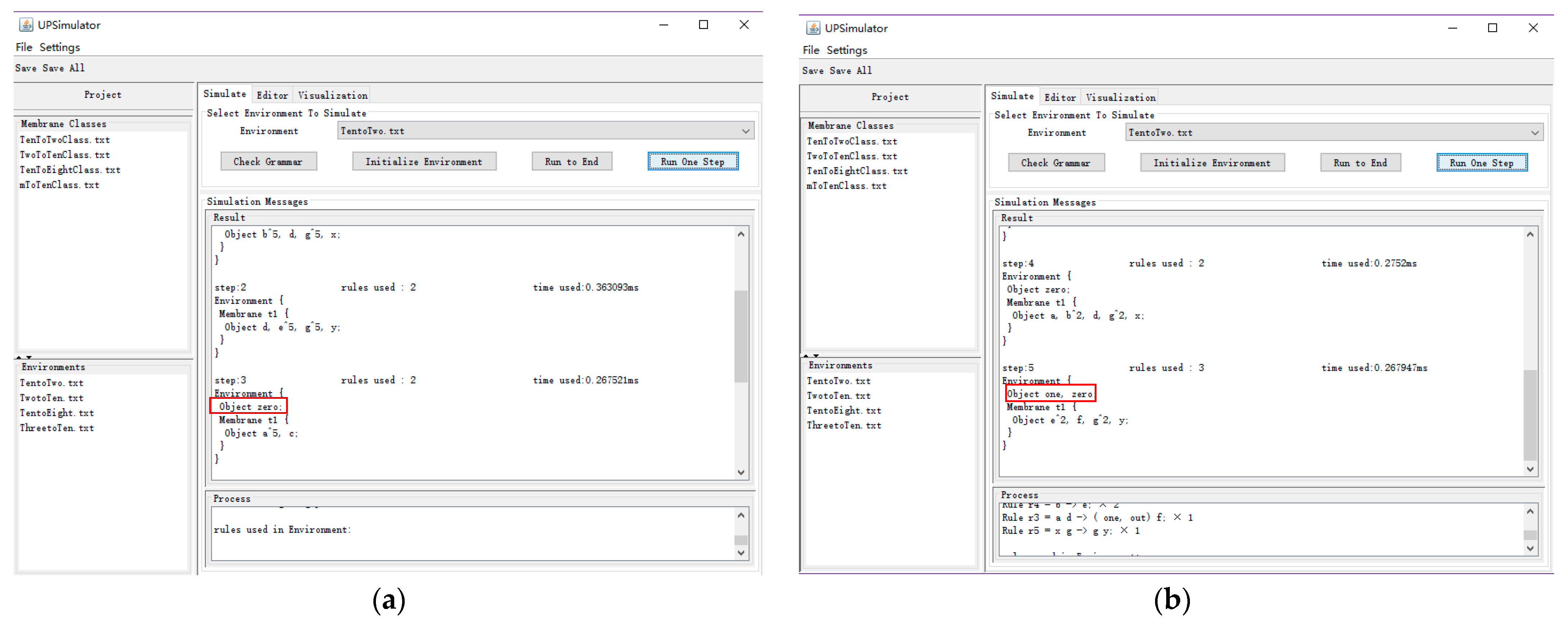
5.1. Simulation of Π_{10_2}

We can simulate the given model according to the following steps:

(1) We use UPLanguage to describe the rules in Π_{10_2}. We define a TenToTwo membrane class as follows:

Membrane TentoTwo{

Rule r1 = a^2→b g;

Rule r2 = c→d x;

Rule r3 = a d→f (one, out);

Rule r4 = b→e;

Rule r5 = g x→g y;

Rule r6 = e g→a;

Rule r7 = y d→c (zero, out);

Rule r8 = y f→c;}

In this membrane class, we use zero to represent ‘0’ in binary and one to represent ‘1’ in binary.

(2) The simulation instance is described in UPLanguage. An emulation instance is one in which we define in the environment the objects of the membrane class TenToTwo and the values of the number system conversion (represented by object multisets). For example, the simulation instance that converts the decimal number ‘10’ to a binary number is:

Environment{

Membrane TentoTwo t1{

Object a^10, c;

}

}

where:

‘Object’ is used to specify object multisets used in the simulation. a^10 means the decimal number to be converted is ’10.’ ’c’ indicates the one object c that needs to be put into the environment beforehand when performing the conversion. When the decimal number n needs to be converted to binary, simply change ‘a^10’ to ‘a^n’ in the environment description above.

We import the above descriptions of the membrane class and environment into the UPSimulator. In Figure 7a, Figure 7b, Figure 7c, and Figure 7d respectively represent the generation of the 1st, 2nd, 3rd, and 4th bits of binary numbers. After running UPSimulator, it generates the first ‘0’ in the third time slice, shown in Figure 7a. The second ‘1’ is produced in the fifth time slice, shown in Figure 7b. Figure 7c shows that the third ‘0’ is generated in the ninth time slice. The fourth ‘1’ is generated in the 11th time slice, displayed in Figure 7d. The conversion process took a total of 11 time slices.

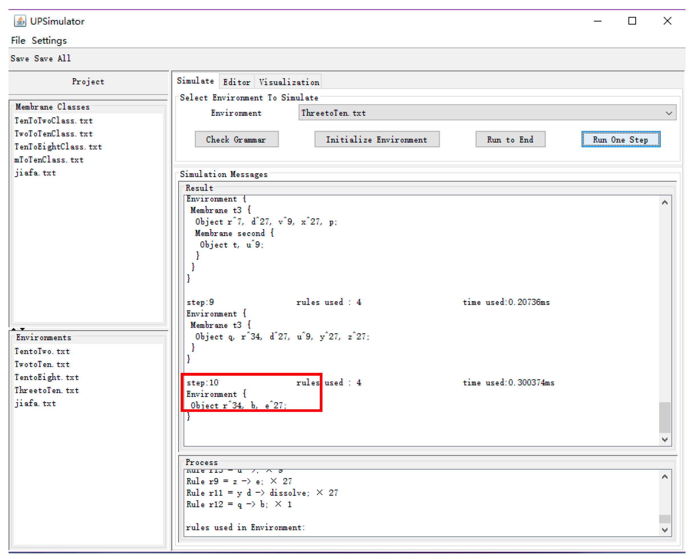
5.2. Simulation of Π_{m_10}

Follow the steps below to simulate Π_{m_10}:

(1) For the simulation of Π_{m_10}, the model is described in UPLanguage, and since the simulation is a 4-bit 3-digit number, a trinary to decimal membrane class is defined and written to the file mToTwoClass.txt.

Membrane ThreetoTen{

Rule r1 = zero b→p x^27 c^27 (t, in second);

Rule r2 = one b→p x^27 d^27 (t, in second);

Rule r3 = two b→p x^27 d^27 (p x^27 d^27, in second);

Rule r4 = e→v (u, in second);

Rule r5 = c v→c z^3;

Rule r6 = d v→d z^3 r^3;

Rule r7 = x→y;

Rule r8 = p→q;

Rule r9 = z→e;

Rule r10 = c y→dissolve;

Rule r11 = d y→dissolve;

Rule r12 = q→b;

Rule r13 = u→;

Membrane second{

Rule r1 = d u→d (r^3, out);

Rule r2 = x→y;

Rule r3 = p→t;

Rule r4 = y d→;

Rule r5 = t→dissolve;

}

}

(2) The simulation instance is constructed, and the nested membrane class ThreetoTen is placed into the environment, with the first ‘1’ and ‘a’ being executed first, and then the remaining bits are executed sequentially from the inside out. The code structure of the 4-bit ternary number ‘1021’ when executed in UPSimulator is as follows:

Environment{

Membrane ThreetoTen t3{

Object one;

Membrane ThreetoTen t2{

Object zero;

Membrane ThreetoTen t1{

Object two;

Membrane t{

Object one,a;

Rule r1 = zero a→b e dissolve;

Rule r2 = one a→b e r dissolve;

Rule r3 = two a→b e r^2 dissolve;

}

}

}

}

}

(3) Finally, the result is marked in a red frame, as shown in Figure 8. There are no new inputs in the system after the end of the 10th time slice. The quantity of r is 34 at this time, so the converted decimal number is 34, and it took a total of 10 time slices.

6. Final Remarks

Membrane computing is a new branch of natural computing and a new computational model. It abstracts biochemical reactions in biological cells and absorbs the principle of high efficiency of complex biochemical reactions in biological cells; each biological cell not only works in parallel but also collaboratively, which greatly improves the working efficiency.

The basic operations of a computer system, whether basic arithmetic operations or complex software systems, cannot be run without number system conversion. This paper describes how to implement the conversion between number systems in the membrane computing framework. The P system for decimal-to-binary conversion Π_{10_2}, the P system for binary to decimal conversion Π_{2_10}, P system for decimal to n-binary Π_{10_m} and the P system for n-bit m decimal to decimal Π_{m_10} are designed, while simulation experiments are carried out with UPSimulator to prove the correctness of its rules. Π_{10_2} and Π_{10_m} are based on the Quotient division method to design rules and implement corresponding functions. Π_{2_10} and Π_{m_10} design rules to accomplish the conversion of binary and m-binary numbers to decimal numbers on the basis of the Positional expansion method, respectively.

In the number conversion P system, using fewer rules or objects to improve the efficiency of number conversion is further work that can be conducted. The conversion between arbitrary binary values is also an issue we need to study in the next step.

References

1. Păun, G. A Quick Introduction to Membrane Computing. J. Log. Algebr. Program. 2010, 79, 291–294. [Google Scholar] [CrossRef]
2. Păun, G. Computing with Membranes. J. Comput. Syst. Sci. 2000, 61, 108–143. [Google Scholar] [CrossRef]
3. Bernardini, F.; Gheorghe, M. Cell Communication in Tissue P Systems: Universality Results. Soft Comput. 2005, 9, 640–649. [Google Scholar] [CrossRef]
4. Păun, A.; Păun, G. Small Universal Spiking Neural P System. Biosystems 2007, 90, 48–60. [Google Scholar] [CrossRef] [PubMed]
5. Păun, A.; Păun, G. The Power of Communication: P Systems with Symport/Antiport. New Gener Comput. 2002, 20, 295–305. [Google Scholar] [CrossRef]
6. Bernardini, F.; Gheorghe, M. Languages Generated by P Systems with Active Membranes. New Gener. Comput. 2004, 22, 311–329. [Google Scholar] [CrossRef]
7. Freund, R.; Martín-Vide, C.; Păun, G. From Regulated Rewriting to Computing with Membranes: Collapsing Hierarchies. Theor. Comput. Sci. 2004, 312, 143–188. [Google Scholar] [CrossRef]
8. Alhazov, A.; Martín-Vide, C.; Pan, L. Solving a PSPACE-Complete Problem by Recognizing P Systems with Restricted Active Membranes. Fundam. Informaticae 2003, 58, 67–77. [Google Scholar]
9. Zeng, X.; Song, T.; Zhang, X.; Pan, L. Performing Four Basic Arithmetic Operations with Spiking Neural P Systems. IEEE Trans. NanoBiosci. 2012, 11, 366–374. [Google Scholar] [CrossRef] [PubMed]
10. Peng, X.; Fan, X.; Liu, J.; Wen, H. Spiking Neural P Systems for Performing Signed Integer Arithmetic Operations. J. Chin. Comput. Syst. 2013, 34, 360–364. [Google Scholar]
11. Zhang, G.; Rong, H.; Paul, P.; He, Y.; Neri, F.; Pérez-Jiménez, M.J. A Complete Arithmetic Calculator Constructed from Spiking Neural P Systems and Its Application to Information Fusion. Int. J. Neur. Syst. 2021, 31, 2050055. [Google Scholar] [CrossRef]
12. Guo, P.; Chen, J. Arithmetic Operation in Membrane System. In Proceedings of the 2008 International Conference on Bio-Medical Engineering and Informatics, Sanya, China, 27–30 May 2008; pp. 231–234. [Google Scholar]
13. Guo, P.; Zhang, H. Arithmetic Operation in Single Membrane. In Proceedings of the 2008 International Conference on Computer Science and Software Engineering, Wuhan, China, 12–14 December 2008; Volume 3, pp. 532–535. [Google Scholar]
14. Yang, R.; Guo, P.; Li, J.; Gu, P. Arithmetic P Systems Based on Arithmetic Formula Tables. Chin. J. Electron. 2015, 24, 542–549. [Google Scholar] [CrossRef]
15. Guo, P.; Luo, M. Signed Numbers Arithmetic Operation in Multi-Membrane. In Proceedings of the 2009 First International Conference on Information Science and Engineering, Nanjing, China, 26–28 December 2009; pp. 393–396. [Google Scholar]
16. Guo, P.; Zhang, H.; Chen, J. Fraction Arithmetic Operations Performed by P Systems. Chin. J. Electron. 2013, 22, 689–694. [Google Scholar]
17. Guo, P.; Zhang, H.; Chen, H.; Liu, R. Fraction Reduction in Membrane Systems. Sci. World J. 2014, 2014, e858527. [Google Scholar] [CrossRef] [PubMed]
18. Guo, P.; Quan, C.; Ye, L. UPSimulator: A General P System Simulator. Knowl. Based Syst. 2019, 170, 20–25. [Google Scholar] [CrossRef]
19. Păun, G.; Rozenberg, G. A Guide to Membrane Computing. Theor. Comput. Sci. 2002, 287, 73–100. [Google Scholar] [CrossRef]
20. Brisebarre, N.; Lauter, C.; Mezzarobba, M.; Muller, J.-M. Comparison between Binary and Decimal Floating-Point Numbers. IEEE Trans. Comput. 2016, 65, 2032–2044. [Google Scholar] [CrossRef]
21. Song, F. Conversion Rules Between Different Carry Counting Systems. Cyberspace Secur. 2020, 11, 61–63. [Google Scholar]
Figure 1. The structure of a cell-like P system.
Applsci 13 09945 g001
Figure 2. P system for decimal to binary.
Applsci 13 09945 g002
Figure 3. P system for binary to decimal.
Applsci 13 09945 g003
Figure 4. P system for decimal to m-binary.
Applsci 13 09945 g004
Figure 5. P system for n-bit m deciaml to decimal.
Applsci 13 09945 g005
Figure 6. P system for 4-bit 3 decimal to decimal.
Applsci 13 09945 g006
Figure 7. Simulation process from decimal number ‘10’ to binary number ‘1010’.
Applsci 13 09945 g007aApplsci 13 09945 g007b
Figure 8. Simulation result of the 4-bit 3-decimal number ‘1021’.
Applsci 13 09945 g008