P System Design for Integer Factorization

Abstract

Membrane computing is a natural computing branch inspired by the structure of biological cells. The mathematical abstract model of a membrane computing system is called a P System, which is one of the main topics in membrane computing research for the design and verification of a P System. Integer factorization is still a world-class problem and a very important research direction. If a fast method can be found to solve the integer factorization problem, several important cryptographic systems including the RSA public key algorithm will be broken. The aim of this paper is to design a P System capable of implementing integer decomposition, taking advantage of the characteristics of parallelism of P Systems. We construct a process with a main goal to study the modal exponential function f(x) = a^x mod N and explore the possible periodic behavior for different values of a. We attempt to compute nontrivial prime factors by the period found and constrain the operation of the P System in polynomial time.

1. Introduction

Membrane computing is a computational model abstracted from the function and structure of biological cells and is formally defined as a P system, first proposed by Păun in 1998 [1]. It is a novel and efficient parallel computing model based on the observation and abstraction of biological cell properties and their internal biochemical reactions. Membrane computation models are divided into three categories: the cell-like P system [2,3], the tissue P system [4], and the neural P system [5].

Cell-like P systems are the most fundamental membrane systems and the first P systems to be proposed. The Cell-like P system is a computational model that simulates the structure and function of cells with parallel and non-deterministic characteristics and it is widely used in the research of computational theory and related fields.

The tissue-type P system is a computational model inspired by protein channels that have intercellular communication, which processes symbols in a network of cells in a multiset rewriting fashion. Each cell has a finite state memory, handles multiple sets of symbolic pulses, and can send pulses (“excitation”) to neighboring cells. This network of cells proved to be quite powerful; even when using a small number of cells, they could simulate a Turing machine.

Neural P systems are a class of pulsatile neural P systems (referred to as SN P systems) based on the idea of spiking neurons in neurobiology, in which time (when a neuron fires and/or spikes) plays an important role. For example, the result of the calculation is the time between the moments when the specified neuron discharges spikes.

Membrane computing has been shown to be theoretically Turing-complete [6], i.e., it can be used to solve any Turing-computable problem. The advantage of membrane computing is that it is highly parallel, fault-tolerant, and scalable [7] and can be applied to various fields such as biology, mathematics, and computer science. In the paper [8], a membrane computing framework based on biological systems was proposed, and the proposed framework was simulated and evaluated to verify the superiority of membrane computing methods. The literature [9] combined cell-like P Systems with particle swarm optimization algorithms and used them for solving Sudoku problems.

Integer factorization, also known as prime factorization, is a classical mathematical problem that aims to represent a positive integer as a product of prime factors. Given two large prime factors, it is easy to find their product, but it is hard to get a result in the opposite task. This is one of the key problems of modern cryptographic systems. If a fast solution to the integer decomposition problem could be found, several important cryptosystems would be broken, including the RSA Public-Key Cryptosystems [10] and the Blum Blum Shub random number generator. Researchers have been making related attempts, such as GNFS [11] and Fermat factorization [12].

The use of a P system for integer decomposition was studied by Alberto Leporati [13] et al., who proposed three P systems for arithmetic operations. The first P system implements the addition operation to compute two m-bit binary numbers in O(m) steps, and the second P system completes the multiplication operation to compute two m-bit binary numbers in O(mlog m) steps. The third P system implements the first two P systems as subsystems to complete the factorization of m-bit natural numbers in O(mlog m) steps. Takayuki [14] et al. considered asynchronous parallelism in membrane computation and proposed an asynchronous P system that performs two basic arithmetic operations and factorization. Obtułowicz [15] proposed a P system with an active membrane that is capable of polynomial time to solve integer factorization problems. In addition, Zhang [16] et al. provided a linear time P system for the prime factorization problem in the framework of a tissue P system with cell division. Liu [17] et al. proposed an unconstrained time model for solving integer factorization problems with SNP systems.

In 1994, Shor proposed a quantum computer-based polynomial-time factorization algorithm called Shor’s algorithm [18]. Shor’s algorithm is centered on transforming the factorization of large numbers into the period of the solver function. The running time of Shor’s algorithm consists of O(${\left(\log n\right)}^2\times \log \log n$), a quantum computer, and on an electronic computer O($\log n$), it still has better performance than the excellent algorithm on an electronic computer (GNFS, time complexity O(${\mathrm{e}}^{\mathrm{c}{\left(\log n\right)}^{1/3}\times {\left(\log \log n\right)}^{2/3}}$). The superiority of the shor algorithm comes not only from its parallel computing capability during function cycle computation, but it also stems from the properties of quantum measurements. Based on the maximal parallelism of evolutionary rule execution in the membrane computation model, our research attempts to design a cell-like P system for solving factorization problems, the core of which lies in designing a P system for solving period problems.

The remainder of this study is structured as follows: In Section 2, we give a brief description of the cell-like P system and an introduction to the theory related to integer factorization. In Section 3, we introduce algorithms for integer factorization. In Section 4 and Section 5, we propose the design of P systems for integer factorization and provide examples. Finally, Section 6 provides a summary and outlook for further research.

2. Foundation

2.1. Cell-like P System

In this section, we briefly introduce a basic model of a cell-like P system. The cell-like P system consists of membranes, intra-membrane objects, and intra-membrane evolutionary rules. Membranes labeled by different labels form the basic structure of the cell-like P system through nested structures. The outermost membrane, called the skin membrane, serves to delineate the entire membrane system from the external environment. When the membrane contains no other membrane, it is called an elementary membrane, otherwise, it is called a non-elementary membrane. In this paper, we do not strictly distinguish between elementary and non-elementary membranes, and we refer to them collectively as membranes. The data are represented by the number of objects inside the membrane and the objects are evolved by evolutionary rules. The evolutionary rules can not only change the number and type of objects, but also transport the objects between different membranes and make the membrane divide and dissolve. For example, in Figure 1, a structure consisting of four membranes is shown. Among them, Skin represents the skin membrane. In addition to the Skin membrane, we refer to the membranes numbered 2 and 3 as elementary membranes, while the membrane numbered 1 is a non-elementary membrane. The non-elementary membrane 1 contains two objects a and membrane 3, while membrane 3 contains object b, while membrane 2 does not contain any object.

The computation of cell-like P systems is performed by evolutionary rules, which are defined as rewrite rules for membranes and objects. All objects and membranes can evolve according to the evolution rules. If there are no evolutionary rules applicable to any object, the system stops computation. A cell-like P system of the degree m can be defined formally as follows:

$$\mathsf{\Pi }=\left(O,\mu ,{\omega }_1,\dots ,{\omega }_m,R_1,\dots ,R_m,{{\rho }_1,...,{\rho }_m,i}_o\right)$$

(1)

where O is the alphabet of the system, representing the set of so objects used in the system. $O^{\ast }$ is the set of strings that can be constructed using the symbols in O. Each multiset can be represented by a string, where λ denotes the empty string and $O^{+}=O^{\ast }-\left\{\mathsf{\lambda }\right\}$;

μ is the membrane structure composed of m membranes, where each membrane is assigned a label to refer to itself;

${\omega }_i\left(1\le i\le m\right)$ denotes the multiset of objects in membrane i in the initial state. The statement that ${\omega }_i$ = $\lambda$ means that there is no object in membrane i. For instance, in Figure 1, ${\omega }_{Env}=\mathsf{\lambda },{\omega }_1=a^2,{\omega }_2=\mathsf{\lambda },{\omega }_3=b$;

$R_i\left(1\le i\le m\right)$ is the set of evolution rules in membrane i. The representation of the intramembrane rule is $u\to v$ or $u\to v\mathsf{\delta }$, where $u\in O^{+}$, $v\in \left(O\times Tar\right)$, $Tar=\{here,i{n}_j|1\le j\le m,out\}$. Tar indicates the membrane to which the target object v will be sent; here means to stay in the current membrane, $i{n}_j$ means that v will be sent to membrane j, and out means that v will be sent to the outside of membrane i (the father membrane of membrane i). The symbol $\mathsf{\delta }$ represents the membrane dissolution operation. After the membrane is dissolved, the objects in the membrane automatically flow into their parent membrane. It should be noted that the $\mathsf{\delta }$ operation cannot be performed on the skin membrane;

${\rho }_i\left(1\le i\le m\right)$ defines the partial order relationship of the rules in $R_i$. In this paper, the partial order relationship is shown in the form of priority; that is, the number after the rule is the priority of rule execution, and the smaller the number, the higher the priority, and 0 is the highest priority. For example, the priorities of rules $a\to b,1$ and $c\to d,2$ are one and two, respectively.

i_o is the label of the membrane that holds the system output results.

In the P system, the rules are implemented according to the following conventions:

• The system has a global clock to coordinate the synchronized execution of evolutionary rules, and the timing unit is the time slice;
• Non-deterministic. Suppose n rules compete for objects that can only support k (k < n) rules, then the choice of these k rules is uncertain;
• Maximum Parallelism. At any moment, all executable rules must be executed. In other words, all executable rules are executed in parallel in each time slice of the computation;
• The execution of any rule requires and takes only one time slice. In particular, in a time slice when a rule can be repeatedly executed multiple times, the multiple executions of the rule are also completed in one time slice, i.e., the multiple executions of the rule are parallel.

For convenience, the remainder of this paper will refer to the cell-like P system as simply the P system.

2.2. Integer Factorization

Integer decomposition, as a classical mathematical problem, has applications in mathematics, cryptography, and computer science. Finding efficient algorithms has been the goal of research pursuits. Examples are the GNFS, Fermat method, and Shor algorithm.

Let the greatest common factor of the integers m and n be gcd(m, n). Evidently, gcd(m, n) is a factor of n. For a given positive integer N, the number of integers that are mutually prime with N and less than N is written as φ(N) (called the Euler function). We can obtain

Theorem 1. (Euler’s theorem). 

Suppose 0 < a < N, a and N are mutually prime, then: $a^{\phi \left(N\right)}\mathit{\equiv }1\left(\mathrm{mod}N\right)$. i.e., $a^{\phi \left(N\right)}\%N=1$.

Let f(x) = $a^x\mathrm{m}\mathrm{o}\mathrm{d}N$. By Theorem 1 we have: f(φ(N)) ≡ 1 (mod N). If there exists an even number r such that f(r) = 1, then we have

$${{(a}^{\frac{r}{2}})}^2-1\equiv 0\mathrm{m}\mathrm{o}\mathrm{d}N,$$

(2)

i.e.,

$${(a}^{\frac{r}{2}}+1){(a}^{\frac{r}{2}}-1)\equiv 0\mathrm{m}\mathrm{o}\mathrm{d}N,$$

(3)

when $a^{\frac{r}{2}}\ne 1$, gcd($a^{\frac{r}{2}}-1,N$) and gcd($a^{\frac{r}{2}}+1,N$) cannot both be 1, from which a factorization of N can be obtained. From this we can achieve

Theorem 2. 

Suppose 0 < a < N, a and N are relatively prime, f(x) = a^x mod N. If there is an even number r > 0 such that f(r) ≡ 1 (mod N), then nontrivial factors of N can be obtained by computing gcd($a^{\frac{r}{2}}+1,N$) and gcd($a^{\frac{r}{2}}-1,N$).

2.3. Extended P System

In this subsection, we present further extensions of the P system: membrane permeability [19], promoters, and inhibitors [20]. Indeed, the further expansion does not consider adding further features to the symbol–object membrane system, but rather adding some constraints.

There are other ways to control the passage of an object across a membrane, such as controlling the permeability of the membrane. Indeed, the permeability of biological membranes is variable. In membrane systems, permeability is controlled by using a τ behavior that is the opposite of the δ behavior. The rules associated with this behavior have the same form as δ; the rule is shaped like u → vτ, where u and v are strings denoting a multiset of objects, and the objects in v are associated with various target commands so that δ and τ cannot be associated with the same rule. The effect of such rules is to increase the “thickness” of the membrane so that it cannot be penetrated.

Assume that all membranes have a thickness of 1 in the initial grid (the rest of the paper also defaults to a membrane thickness of 1). If a rule is used in one of the membranes and produces the symbol τ, then the thickness of the membrane becomes 2. A membrane of thickness 2 can no longer be increased in thickness by another rule that produces the symbol τ and, furthermore, no object can pass through it. If the rule that produces the character δ occurs in a membrane of thickness 2, then the thickness of that membrane becomes 1, therefore, the membrane is permeable in the next step. If the rule produces both δ and τ in the same membrane and in the same step, then the thickness of the membrane remains unchanged. The cumulative effect of δ and τ is shown in Figure 2 (the numbers in the two circles indicate the thickness of the membrane).

Biochemical reactions in organisms occur collaboratively, so many reactions in cells are enhanced by enzymes. The role of enzymes and the role of catalysts can be realized by the rules of catalysis. The presence of a chemical that makes it possible (or makes it more likely) for a biochemical reaction to occur is not a catalyst; it can evolve separately and evolution can proceed in parallel with the reaction it facilitates. The same can be said about inhibitors, which are chemicals that block certain reactions (they bear no resemblance to catalysts and have a negative effect on the reaction).

Formalize this idea by considering the use of facilitators or inhibitors at each rule level, i.e., consider rules of the form u→v|_a and u→v|_⌐a, where a is an object. Suppose that in region i’ we have the object multiset ω’ and the rule u→v|_a can be used only if object a belongs to the multiset ω’-u, and the rule u→v|_⌐a can be used only if object a does not belong to the multiset ω’-u. That is, it is the facilitator or inhibitor object that should appear or not appear in the region where the rule is used.

In this article, Section 3 will design a parallel algorithm to compute r, and Section 4 will design a P system for integer factorization and use these extended P system rules.

3. Integer Factorization Algorithm

This section discusses the key algorithms for integer factorization and proves the correctness of the algorithms. In this paper, we only consider the problem of decomposing a large number N into two prime factors.

3.1. Periodic Function

In order to efficiently obtain an even r in Section 2.2, we first discuss the properties of the function f(x).

Theorem 3. 

For integers a, N (N > a > 0), if gcd(a, N) = 1, then f(x) = $a^x$ mod N is a periodic function on the domain of positive integers.

f(x) is a periodic function with period φ(N). Since f(0) = 1, we have

Theorem 4. 

Suppose $f\left(x\right)=a^x\mathrm{mod}N,x\ge 0$, if the integer r > 0, f(r) = 1, and $f(u)\ne 1$ for any integer u < r and u > 0, then r is a minimum period of f(x).

For N > 4, although the minimum period r of f(x) cannot be guaranteed to be even, we have

Theorem 5. 

For N > 4, gcd(a, N) = 1$,f\left(x\right)=a^x\mathrm{mod}N,x\ge 0$, then f(x) must have an even period.

In summary, there must be an even number of periods of f(x).

3.2. Parallel Algorithm for Integer Factorization

Based on the calculation of even periods of f(x), we obtain an integer factorization algorithm PFLN such as Algorithm 1. When a satisfies gcd(a, N) = 1 (the gcd algorithm for solving the greatest common divisor uses the Euclidean algorithm [21]), call the algorithm FMEP&PF (Algorithm 2) to find the period of f(x) and the factorization of N. When p ≠ 1 (Line 4), it means to find the factorization of N, output p and q (line 5), and end the loop of Line 2~8 (line 6). Line 9 is used to end the whole process of finding the factorization (all parallel computation processes). When p = 1, increase the value of a and continue the loop line 2~8. In Section 4, we will design the P system to implement different values of a so that FMEP&PF(a, N, p, q) are executed in parallel in different membranes. When any FMEP&PF call in the parallel execution and has a return value, it will make p ≠ 1, thereby outputting a factorization of N and ending the whole solving process.

Algorithm 2 provides the procedure for computing the factorization for a determined value of a. From Theorem 5, it is clear that the while loop started by line 2 always ends at some r value by the instruction of line 10. On the other hand, the initial value of r is 2 (line 1), and the value of r is increased by 2 for each loop to ensure that the minimum even number of periods can be obtained. Thus, by Theorems 2–5, we prove the correctness of Algorithm 2.

In Algorithm 2, we find the minimum even period r of f(x) when the condition in line 3 is satisfied. Lines 4 to 9 provide the procedure for factoring p and q by computing gcd($a^{\frac{r}{2}}-1,N$) or gcd($a^{\frac{r}{2}}+1,N$). Line 10 returns p and q and ends the algorithm run.

Algorithm 1 Prime Factorization Algorithm for Large Numbers (PFLN)

Input: N; // An integer N > 4

Output: p, q; // (p×q = N)

procedure PFLN (Number N)

p ← 1, q ← 1; for $a\leftarrow 2$to N do // For a different a, perform the following operations in parallel.   If gcd($a,N$) == 1 then FMEP&PF(a, N, p, q);    // Perform factorization on a different a in parallel.   if p ≠ 1 than // Factorization of N found     print(p, q);     break;   end if end for exit // End all parallel factorization processes end procedure

Algorithm 2 FMEP&PF // Finding the minimum even period and the prime factor

Input: a, N;

Output: p, q;

$r\leftarrow 2$; while(1) do   if ($a^r$– 1) % N == 0 than     $p\leftarrow \mathbf{g}\mathbf{c}\mathbf{d}(a^{\frac{r}{2}}+1,N)$;     if p ≠ 1 than q = N / p;     else       $p\leftarrow \mathbf{g}\mathbf{c}\mathbf{d}(a^{\frac{r}{2}}-1,N)$;       q = N / p;     return p and q;   end if   $r\leftarrow r+2;$ end procedure

4. P System Design of Integer Factorization

4.1. Definition of P System for Integer Factorization

We give the definition of the P system ${\mathsf{\Pi }}_{\mathit{IF}}$ that can complete the factorization as follows:

$${\mathsf{\Pi }}_{IF}=\{O,\mu ,{\omega }_{Skin},{\omega }_{Com},{\omega }_{GCD},R_{Skin},R_{Com},R_{GCD},{\rho }_{Skin},{\rho }_{Com},{\rho }_{GCD},i_o\}$$

(4)

where:

• O = {ξ^N, a, b, c, d, e, f, g, h, i, k, ξ₁, ξ₂, p, q, q₁, q₂, r, v, w, w’, y₁, y₂, y₃, y₄, z, z₁, z₂}, where N refers to the size of the number to be decomposed;
• μ = [[[ ]_GCD1 [ ]_GCD2]_Com]_Skin;
• ω_Skin = λ, ω_Com = { a, d², ξ^N }_, ω_GCD = λ;
• R_Skin = λ;
  R_Com = {$a\to {\left[b\right]}_{\mathit{Com}}{\left[c{r}^2\right]}_{\mathit{Com}};d\to q;b\to ad;q\to {z|}_{cr};$ z → z₁ z₂|_c; c → d; z₁ → z z₁|_z2; d z₂ → d; d → e|_¬z2; z₁ → y y₂|_e; z → v z₂|_e; e → c; v c → p f, 1; vⁿ → λ, 2; v → i f, 3; f → z₁|_i; p → g h|_i; y → y₁|_i; i → λ; z₁ → z z₁|_z2; g z₂ → g q₁, 1; y₁→ y y₁|_y2; h y₂→ h q₂, 1; g→ w r², 2; h→ λ, 2; z→ v|_w; q₁→ z₂|_w; z₁→ λ|_w; q₂→ y₂|_w; y₁→ λ|_w; w→ c; p→ τ w’(k, out)|_¬i; y → y₃ y₄|_{⌐v ⌐i}; y₃→ (in GCD₁); y₄→ (in GCD₂); ξ → ξ₁ ξ₂; ξ₁→ (in GCD₁); ξ₂→ (in GCD₂);}; R_GCD = λ;
• The priority of the rules in ${\rho }_{\mathit{Computer}}$, …, ${\rho }_A$ can be seen in the rules in R_Compute, …, R_A.

The execution of the system can be divided into two main phases: the first phase is the splitting of the sub-task membranes for computing different a $(2\le a<N)$, and the second phase is the execution flow for computing the membranes corresponding to a certain a, as shown in Figure 3. In the first stage, a new submembrane is generated every two-time slice, and in this submembrane, a certain object corresponds to a different value of a (e.g., in Figure 3a, d³ represents the membrane corresponding to a = 3 in this membrane). The second stage is to find a period r corresponding to a by splitting the computational membrane in the membranes corresponding to the different values of a generated in the first stage. When a matching period r is found, ${a^{\frac{r}{2}}}^{}-1$ and ${a^{\frac{r}{2}}}^{}+1$ are calculated and the two sets of maximum conventions are also calculated by creating new GCD membranes, respectively, and the result obtained is the final decomposition. It is important to note that the execution of the rules in the membranes corresponding to the different values of a do not interfere with each other (only when the final result is computed in the membrane corresponding to a certain a does the membrane release an abort signal and, thus, the whole system stops working). In other words, the execution of the system is parallel. We will show this process in detail next.

The system performs according to the rules in Figure 4.

4.2. Rules and Procedures for Integer Factorization of P Systems

4.2.1. Main Process

We realize this process through the stacking of compounds and splitting of membranes in the theory of membrane computation and divide the phases of the execution of the P system into two main parts: the splitting process and the computational process. We first construct a modulo exponential function f(x) = a^x mod N. The split process consists of the initial membrane continuously splitting out submembranes dealing with specific values of a (arithmetic iteration of a) to take care of the specific computation, which we refer to as the computational membrane, and the split process is shown in Figure 3a. Inside the computational membrane, i.e., to the computational stage, as shown in Figure 3b, the computation of multiplication and modulo (arithmetic iteration over x) is accomplished by adding value to and reducing specific objects. Inside the computational membrane, the final stage of the computation is determined by an arithmetic determination of f(0) = f(x₁) = 1 by the presence or absence of a flagged object, and if it is true, then the system stops and sends a given number of objects y (representing a₁^r1/2, |y| = a₁^r1/2) and objects ξ (N in ξ^N stands for the number being factorized) into the two GCD membranes to complete the computation of the prime factors.

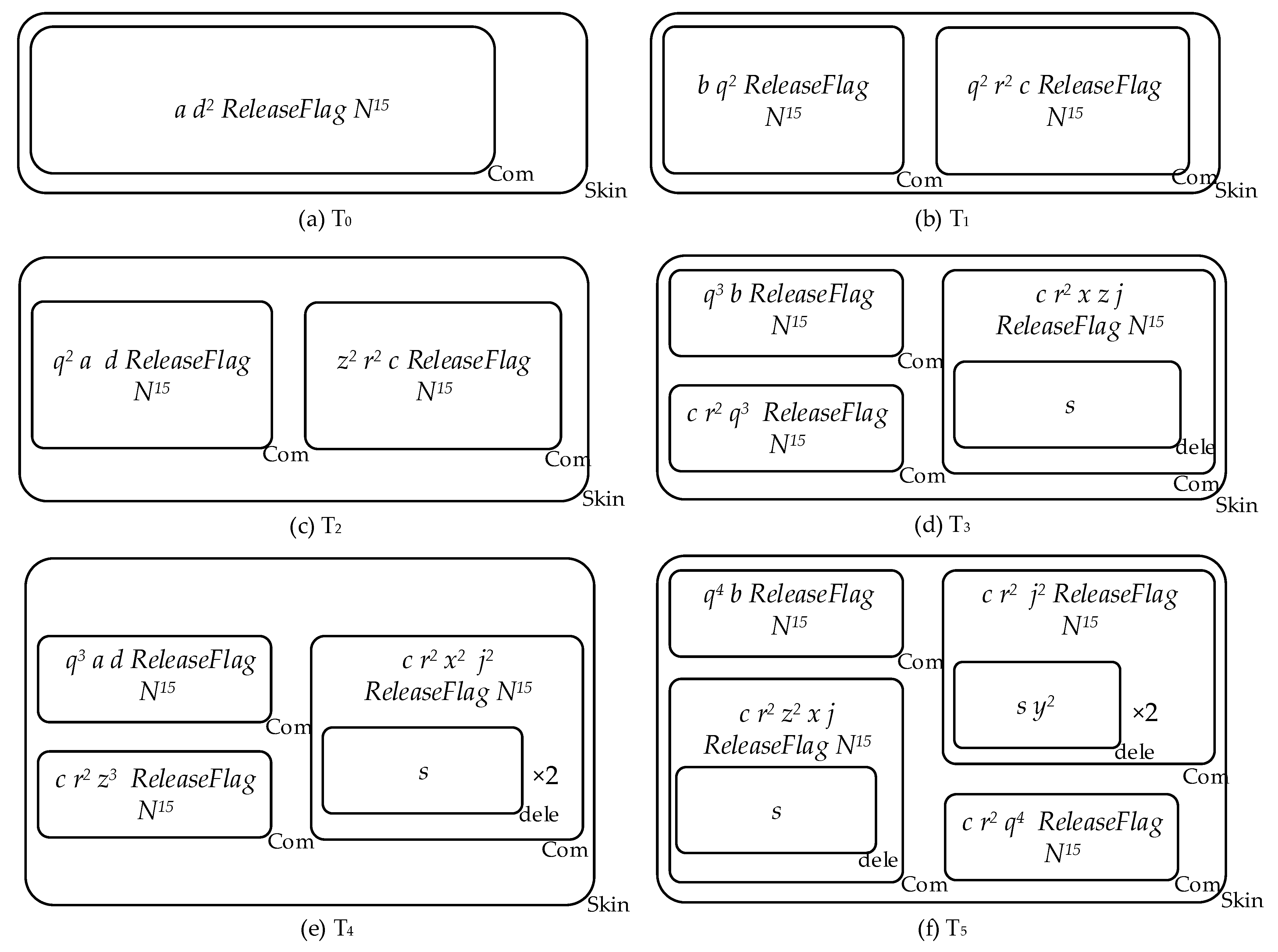
4.2.2. Flag Objects and Their Life Cycle

The computation of the number of theoretic problems also has a specific linear process, but biological computation possesses a parallel mechanism, so we have achieved the realization of rules at specific steps by distinguishing between multiple iconic objects as triggering objects for the rules. For example, if object c is the one we set at the membrane splitting stage, if object c does not appear within the membrane, then the rule responsible for the computation will not be used. The modal exponential function requires multiple rounds of arithmetic iterations for the values of the exponent (e.g., 3², 3⁴, 3⁶), so in the process we have designed, there is a corresponding set of rules that are responsible for consuming and generating the object c. In each round of iterative computation of the modal exponential, the computation of the object c destroys once and then generates once, thus, realizing the loop of one iteration and starting the next one.

We refer to this process as the life cycle of the flag object during the loop. The flag object’s lifecycle approximates the structure of the loop in the algorithm’s design. We use this feature cautiously to ensure that no more than one layer of nested loops occurs, introducing a new exponential time consumption.

4.2.3. Splitting and Calculation Process

As shown in Figure 4, in the initial stage of the system, there is only one initial Com membrane in the Skin membrane that serves as the basis for membrane division. The Com membrane holds the objects a, d², and ξ^N, where the object a can control the splitting process, the object d is responsible for counting, and the count of the object ξ is used as the number to be factored (e.g., if the number to be factored is 25, the number represented by N in ξ^N is 25). The initial Com membrane holds the object a as the flag object of the splitting process (i.e., it has the ability to split), and subsequently splits into two daughter membranes by rule a→[b]_Com[c r²]_Com, where the former will be reduced to an initial membrane with the ability to split by rule b → a d, and will achieve an additional object d than its parent. The latter will be transformed into a computational membrane by rule d → z into a computational membrane, where the count |z| of the object z is the value of a taken in the current modal index a^x mod N. This means that each time a computational submembrane is split out, the initial membrane is restored and receives an increase in count, which is reflected in the object size of the computational submembrane produced at the next split.

Take for example the computational submembrane responsible for computing the modal index 3^xmod 25 (i.e., N = 25, a = 3). After the appearance of object c in the computational submembrane, it proceeds to the next process to compute the value associated with the modal index, which is split by the initial membrane holding objects c, r², z³, and N²⁵. Objects c and r have a fixed number (i.e., 1 object c and 2 objects r), and they are the flagged objects controlling the computational process. The number of objects z |z| is used to indicate the bottom number in the current arithmetic. In the current calculation, the base number is 3, for which 3 objects z produce equal copies under the rule z→z₁ z₂|_c;c→d, that is, 3 objects z₁ and 3 objects z₂, as well as 1 additional object d. To implement the exponential calculation, we use some tricks; that is, the rule z₁→z z₁|_z2; d z₂→d; which, under the action of this rule, will produce |z₂| rounds of computation based on the number of objects z₂, the object d produced in the previous rule is used to ensure that each round of computation will consume 1 and only 1 object z₂ and produce |z₁| object z. That is, after all, the objects z₂ are consumed, the submembrane will be computed to obtain |z₁| × |z₂| object z; that is, a multiplicative computation is completed, and the number is indicated by the newly produced object z’s count |z| denoted by the number of newly generated objects z. In this example, |z| = 3² = 9.

Since the final exponent used to compute the greatest common divisor is a^r/2 instead of a^r, there are two additional rules: d→ e|_⌐z2; and z₁→ y y₂|_e; z→ v z₂|_e;e→ c; which are used to obtain ar along with a^r/2, avoiding the need to do additional root operations in future phases of the submembrane. Moreover, it will transform the object z all into the object v, thus, serving as the flag object for the next stage.

Once we have obtained the iconic object c and object v, we can perform the first modulo determination operation, which is accomplished by three rules, rule v c→p f,1 and rule vⁿ→λ,2, and rule v→i f,3. In the 3^x mod 25 arithmetic of this example, this set of rules performs an integer multiples |N| divisor computation of 3^x − 1, with the final remainder represented by object i. The final remainder is denoted by object i.

If the count of object i is 0, it means that 3^xmod 25 = 1, which satisfies the determination of f(0) = f(x₁) = 1, and it can be submitted to the GCD membrane for calculating prime factors. If the count of object i is not 0, it means that the arithmetic is not satisfied and it goes to the next round of exponential iteration. The new round of exponential iteration is jointly accomplished by six rules, namely rules f→z₁|_i; p→g h|_i; y→y₁|_i; i→λ; rules z₁→z z₁|_z2; g z₂→g q₁, 1; and rules y₁→y y₁|_y2; h y₂→h q₂, 1; rules g→w r², 2; h→λ, 2; rules z→v|_w; q₁→ z₂|_w; z₁→λ|_w; and rules q₂→y₂|_w; y₁→λ|_w; w→c are composed. These six rules continue to iterate over the object |z| = 3² and the object |y| = 3¹, creating 3²⁺² new objects z and 3¹ new objects y. At the end of this set of rules, we obtained the flag object c and the flag object v again, and then performed a modulo judgment.

For this reason, we made the complete process of splitting the membrane and computing the submembrane under the standard execution process into a calculation table based on timing and rounds. For more information, refer to

Table 1. Timing table of main objects during split.

Number of Rounds	Time Slip	Objects in the Membranes
Round 1 (calculate the case of |z| = 2)	T0	a d2
	T1	b d2	c r2 d2
	T2	b z2	c r2 z2
	T3	a b z2	c r2 z2
Round 2 (calculate the case of |z| = 3)	T0	a b d2
	T1	b d z2	c r2 d z2
	T2	b z3	c r2 z3
	T3	a d z3	c r2 z3
Round 3 (calculate the case of |z| = 4)	T0	a d z3
	T1	b d z3	c r2 d z3
	T2	b z4	c r2 z4
	T3	a d z4	c r2 z4

and

Table 2. The timing diagram of the calculation phase (taking N = 25 as an example, processing the timing diagram when a = 3).

Rules	a2×1(32)	a1(31)	a2×2(34)	a2(32)
	c r2 z3
z → z1z2|c; c → d;	d r2z13z23
z1 → z z1|z2; d z2 → d;	r2z9z13d
d → e|¬z2;	r2z9z13e
z1→ y y2|e; z → v z2|e; e → c	r2c v9z29	y3 y23
v c → p f, 1;	r2p f v8z29	y3 y23	r4, p, f, v80, z29	y9, y23
vn → λ, 2;	r2p f v8z29	y3 y23	r4, p, f, v5, z29	y9, y23
v → i f, 3;	r2p f9i8z29	y3 y23	r4, p, f6, i5, z29	y9, y23
f → z1|i; p → g h|i; y → y1|i; i → λ;	r2g z19z29	h y13 y23	r4, g, z16, z29	h, y19, y23
z1 → z z1|z2; g z2→ g q1, 1; y1→ y y1|y2; h y2→ h q2, 1;	r2g z81z19q19	h y9y13q23	r4, g, z54, z16, q19	h, y27, y19, q23
g→ w r2, 2; h→ λ, 2;	r4w z81z19q19	y9y13q23	r6, w, z54, z16, q19	y27, y19, q23
z→ v|w; q1→ z2|w; z1→ λ|w; q2→ y2|w; y1→ λ|w; w→ c	r4c v81z29	y9y23	r6, c, v54, z29	y27, y23

.

5. Cases and Experiments

5.1. Instance of UPLanguage

The UP Simulator [22] simulator uses a new universal P system description language, UPLanguage, which is a superset of the standard P system rules. Based on UPLanguage, we developed a complete experimental code for integer decomposition P systems and wrote a set of UPLanguage rules for handling the highest common divisors. UPLanguage provides some very useful mechanisms, and when writing the experimental code, without destroying the integrity of the partitioning process, we adapted some of the rules, confusing object naming and the design for optimization and compatibility purposes.

The rules adopted in this section are described using UPLanguage, which is specially used for the implementation of simulation. You can find this complete usage case at https://github.com/CqNatural/p-system-integer-factorization (accessed on 20 July 2023).

5.2. Cases

To better understand the rules in Section 4, we rewrite our rules using UPLanguage and simulate them using UPSimulator. Next, we show the process of integer factorization in detail using N = 15 as an example.

At T₀, as shown in Figure 5a, the only objects in the membrane are a d² ReleaseFlag N¹⁵. At the moment of T_1, the execution of the rules a → [b] [c,r²] and d → q cause the membrane to split a new membrane as shown in Figure 5b. At the moment T_2, the rules b → a d and q → z|_{c r} are executed and the objects in the membrane are shown in Figure 5c. Then, at the moment T₃, the rules d → q, a → [b] [c,r²], c z → c x j Delegate:delegate{s} are executed and a new membrane is split, while a new delegate membrane containing the object s is created in the first split membrane as shown in Figure 5d. At the moment T₄, b → a d, q → z|_{c r}, c z → c x j Delegate:delegate{s} is executed again, and the result is shown in Figure 5e. Then, at the moment T₅, the execution of rules a → [b] [c,r²], d → q makes a new membrane split again, and the rule x → (y, in all)|_!z is executed in the first split membrane, as shown in Figure 5f.

At the next time slice T₆, as shown in Figure 6a, the rules b → a d, ReleaseFlag → (DissolveFlag, in all)|_{!z !x j}, c z → c x j Delegate:delegate{s}, q → z|_{c r}, and the rule s y → s SubCompute:subComputee{} in the delegate membrane class are executed.

Since each computer membrane is operating in parallel, in order to save space, in the following pages we only show the computer membranes that were split for the first time, that is, the membrane corresponding to a = 2, as shown in Figure 6b. It shows that at time T₇, the execution of the rule s y → s SubCompute:subComputee{} causes a subComputee submembrane to be generated again. At time T₈, the rule s DissolveFlag → (t, in all)$\delta$|_!y in the delegate membrane class executes the generated object t into the submembrane and dissolves the delegate membrane. At the same time, the four submembranes (subComputee membrane) enter their parent membrane (Computer membrane), as shown in Figure 6c. At time T₉, the rule t → (v, out) in the subComputer membrane class is executed, as shown in Figure 6d. Then at time T₁₀, the rules v c → p f, 1 and v → i f, 3 are executed, as shown in Figure 6e. At time T₁₁, the rules p → r² c|_i, 1, f → (t, in all) |_i, 1 and i → λ are executed, as shown in Figure 6f. Then, at time T₁₂, as shown in Figure 6g, the rule t → (v, out) in the SubComputer membrane class is executed, and the object t⁴ in the four submembranes enters the parent membrane, and the obtained v¹⁶ is realized computes the value of (a²)².

Next, at time T₁₃, as shown in Figure 6h, the rules v c → p f, 1 and v¹⁵ → (f¹⁵, here), 2 are executed and the former has a higher priority. As there is an object c, it will be executed first and execute only once, first implementing the operation of calculating a^x−1, and then implementing the calculation of the value of a^x−1mod N, the number of v retained after the execution is a^x−1mod N value, while f is used to restore v to enter the next cycle.

Due to the length of the article, in the following steps, we will only present key step diagrams. At time T₁₄, as shown in Figure 7a, the rule p → w (k, out) (k, in all), 2 is executed, and the generated object k enters the parent membrane Skin membrane and all child membranes, respectively. At T₁₅, the rule k → (k, in all), 1 in the Skin is executed, and the rule k → $\delta$, 2 in the SubComputer membrane class can be executed, dissolving all the SubComputer membranes, as shown in Figure 7b. Then, at time T₁₆, the rule k w → h, 0 is executed.

Next, at time T₁₇, the rule r² → R|_h is executed. At time T_18, the rule R h → cFlag|_!cFlag is executed. At time T₁₉, the rule j cFlag → cFlag SubCompute:subCompute{T} is executed to generate a new subCompute submembrane. At the same time, an object k will be generated in other Computer membranes (not shown here) and enter the Skin membrane, as shown in Figure 7c. At time T₂₀, the rule T → (V, out) is executed, and at the same time the rule k → (k, in all) in the Skin membrane, 1 is executed, sending k to all submembranes, as shown in Figure 7d. At time T₂₁, the rules T → (V, out) and R cFlag → rFlag|_!j are executed. At time T₂₂, the execution of the rule V → P (T, in all)|_rFlag sends the generated T² to all sub-branes. Then, at time T₂₃, the rules P rFlag → cFlag and T → (V, out) are executed, and the generated V⁴ is sent to the parent membrane, as shown in Figure 7e. Then, at time T₂₄, as shown in Figure 7f, the rule cFlag → GCDFlag CalculateFactor:cf1{I} CalculateFactor:cf2{D_}|!R,!r,1 creates two cf1 and cf2 submembranes. At T₂₅, the rules V → (V, in all)|_GCDFlag,2, N → (N, in all)|_GCDFlag,2 and the rule I → V, 1 in the CalculateFactor membrane class are executed, as shown in Figure 7g. At T₂₆, the rule GCDFlag → (GCDFlag, in all)|_{!V !N},3 satisfies the execution conditions and enters into all submembranes and the rule D V → λ in the CalculateFactor membrane class is executed, as shown in Figure 7h.

Then, at time T₂₇, the execution of the rule GCDFlag → $\delta$, 2 dissolves the SubCom membrane and the execution of the rule GCDFLag → Give GCD:g1{}, 2 in the CalculateFactor membrane class generates a new g1 submembrane, and it should be noted here the object c t in the generated g1 membrane is the default object in the GCD membrane class, and the object CreateSunMem in the a1 membrane is also the default object in the A membrane class, as shown in Figure 8a. At time T₂₈, the rules V → (m, in all)|_Give, N →(n, in all)|_Give are executed in the cf1 and cf2 membranes, respectively, and all the objects V⁵ and N¹⁵ are each sent to their submembrane a1 middle. Then, at time T₂₉, the rule m n → g, 1 is executed, and n⁵ is consumed, as shown in Figure 8b. At time T₃₀, the rules g → a b (a b Num, in all), 3 and n → b (a, in all)|_g, 2 are executed in cf1 and cf2 membranes, respectively, as shown in Figure 8c. At time T₃₁, the rules a, b → x, 1 and CreateSubMem Num → A:a{}|_b, 3 are executed, respectively, generating a type A submembrane a in the a1 membrane, as shown in Figure 8d. At time T₃₂, the rules c → y|_x, 1, Num → (Num, in all)|_{!CreateSubMem} are executed. At time T₃₃, the rule a y → a d, 2 is executed. At time T₃₄, the rules x → b|_d, 3 and d → c, 4 are executed, and at the same time, an object k is generated in other Computer membrane classes and enters the Skin membrane. Then, at time T₃₅, the rule a, b → x, 1 is executed, as shown in Figure 8e. At time T₃₆, the executed rule is c → y|_x, 1. At time T₃₇, the rule a y → a d, 2 is executed. At time T₃₈, the rule d → c, 4 is executed, as shown in Figure 8f. At time T₃₉, the rule a, b → x, 1 is executed. At time T₄₀, the rule c → y|_x, 1 is executed. At time T₄₁, as shown in Figure 8g, the rule y → z e, 3 is executed. At time T₄₂, the rule x → (z x, out)|_z, 4 is executed. Then, at time T₄₃, the rule x → (z x, out)|_z, 4 is executed, as shown in Figure 8h.

At time T₄₄, the rules x Give → IsOne and z → $\delta$ (all)|_!x, 4 are executed, and the result is shown in Figure 9a. At time T₄₅, the rule a y → a d, 2 is executed. At time T₄₆, as shown in Figure 9b, the rules x → b|_d, 3, d → c, 4 and f → (DissolveAllCOmpute, out)|_EndFlag are executed. At time T₄₇, the rule a, b → x, 1 is executed, and at the same time, other Computer membranes send an object k to the Skin membrane. Then, at time T₄₈, the rules k → (k, in all), 1, c → y|_x, 1 and DissolveAllCompute →δ|_EndFlag are executed, and all the computer membranes in the system are dissolved at this time. At time T₄₉, the rule y → z e, 3 is executed. At time T₅₀, as shown in Figure 9d, the rule x → (z x, out)|_z, 4 is executed. At time T₅₁, as shown in Figure 9e, the rule x → (x, out) is executed. At time T₅₂, as shown in Figure 9f, the rules x Give → IsOne and z → $\delta$ (all)|_!x are executed. Finally, at time T₅₃, the execution rule is IsOne → x (EndFlag, out), 2, and the execution is over. At this time, x⁵ and x³ in cf1 and cf2 represent the decomposition results of five and three, respectively.

5.3. Experimental Results

When N = 15, the result is shown in Figure 10a. The x⁵ and x³ in the cf1 and cf2 membranes are the decomposition results. When N = 39, the result is shown in Figure 10b, and x¹³ and x³ in the cf1 and cf2 membranes are the decomposition results.

However, we found through experiments that the UPSimulator is prone to overflow problems when dealing with numbers to be decomposed with N > 39, which affects the final accuracy. From the simulator’s point of view, we re-audited the source code part of UPSimulator and found that this is due to a flaw in the initial design of UPSimulator, which did not consider the support for extra-long integer numbers in the data structure. In the P system we designed, the number to be decomposed is represented by the count of the compound object N, which is |N|. This is caused by the fact that the system may produce intermediate number results with long digits when computing the periodic functions, and our P system does not create a new exponential order problem.

We examined some algorithms that already existed and the comparison results are shown in

Table 3. Comparison of space–time complexity of Factorization algorithm.

Algorithm	Time Complexity	Space Complexity
General Number Field Sieve (GNFS)	$O\left(e^{c{\left(\log n\right)}^{1/3}\times {\left(\log \log n\right)}^{2/3}}\right)$	-.1
Shor’s algorithm	O((log n)3loglog n logloglog n)	O(log n)
Pollard’s rho algorithm [23]	$O(\sqrt{n}$)	O(1)
ours(PFLN)	O(nlog n)	O(n) 2

¹ Relatively complex, readers can refer to the article [24]. ² When considering the space complexity of P system, it is often difficult to measure because the number of objects and the number of membranes are constantly changing. In our P system, the best case in terms of space complexity is found in the first iteration of the first split, and the space complexity at this time is O(1). But the best case cannot be used as a measure, so we use the number of membranes as a measure of space complexity, instead of only thinking about it at the algorithmic level. In general, the number of membranes increases linearly with the splitting process, appearing as O(n). We think that the space complexity and time efficiency of modulo–exponential periodicization can be discussed more in future work.

. Due to the parallel nature of P systems, the algorithm designed for our P system can ideally perform the task of periodization of modal exponential functions in parallel. By theoretical calculations, our algorithm has O(nlog n) in time complexity, O(1) in the best case, and unknown in the worst case in space complexity. It is important to note that the polynomial demand of time implies an exponential demand of space, and the membrane structure in the P system consumes additional space while executing in parallel. In the current laboratory situation, biocomputing experiments based on P systems remains impossible, so while we have obtained an exciting result, it will remain a threat to asymmetric cryptography in its current form for quite some time to come.

6. Conclusions

The factorization problem is not “tricky” because it is neither a decision problem nor an optimization problem. It seems to be difficult because no one has been able to find polynomial-time algorithms to solve it so far. That is, no deterministic (or even probabilistic) polynomial-time algorithm is known that can be executed on a Turing machine to solve every possible case. For this reason, factorization is used in many cryptographic applications, the most famous of which is, of course, the public-key cryptosystem RSA.

In this research, we propose a cell-like P system solution ${\mathsf{\Pi }}_{IF}$ for the factorization problem. We imitate the periodic processing of the modular exponentiation function f(x) = a^x mod N in the Shor algorithm. Specify a number to be decomposed N = p × q, and the P system Π_IF will target different values of a in the modular exponentiation function and divide to a different submembrane. A submembrane will try increasing the value of x, and see if f(x) achieves a period r. If a submembrane of the system calculates the period r, then the periodicization of the system is completed, and the process of dividing the submembrane ends. In the last part of the P system, the greatest common divisor will be calculated through the confirmed period r, and the obtained two numbers gcd($a^{\frac{r}{2}}+1,N$) and gcd($a^{\frac{r}{2}}-1,N$) are the final two prime factors p and q for N. However, it is still difficult to implement such systems in a biological sense, so it does not affect the security of existing Cryptography.

We built related codes and experiments in UPSimulator and successfully calculated multiple prime factorization problems including N = 15. Due to how the numerical value of the power calculation increases too fast, UPSimulator overflows when calculating a slightly larger number, making the sample calculation unable to be very large.

Future work can be divided into three parts:

• The membrane structure can continue to be optimized, and a dedicated simulator can be established to test on larger data samples;
• The P system has variants of various biological mechanisms. How to introduce these variants into the current model to improve its performance is worth considering.
• Whether the hit rate of the periodic function has a mathematical law is still a question that can be discussed, which is related to the size of the space when the P system is executed. In this way, it can be determined whether a stable space complexity can be found when performing the integer factorization problem.

References

1. Păun, G. Computing with Membranes. J. Comput. Syst. Sci. 2000, 61, 108–143. [Google Scholar] [CrossRef] [Green Version]
2. Wu, T.; Zhang, Z.; Păun, G.; Pan, L. Cell-like Spiking Neural P Systems. Theor. Comput. Sci. 2016, 623, 180–189. [Google Scholar] [CrossRef]
3. Păun, G. Introduction to Membrane Computing. In Applications of Membrane Computing; Ciobanu, G., Păun, G., Pérez-Jiménez, M.J., Eds.; Natural Computing Series; Springer: Berlin, Heidelberg, 2005; pp. 1–42. ISBN 978-3-540-25017-3. [Google Scholar]
4. Martín-Vide, C.; Păun, G.; Pazos, J.; Rodríguez-Patón, A. Tissue P Systems. Theor. Comput. Sci. 2003, 296, 295–326. [Google Scholar] [CrossRef] [Green Version]
5. Ionescu, M.; Păun, G.; Yokomori, T. Spiking Neural P Systems. Fundam. Informaticae 2006, 71, 279–308. Available online: https://content.iospress.com/articles/fundamenta-informaticae/fi71-2-3-08 (accessed on 26 December 2022).
6. Krishna, S.N. Universality Results for P Systems Based on Brane Calculi Operations. Theor. Comput. Sci. 2007, 371, 83–105. [Google Scholar] [CrossRef] [Green Version]
7. Ibarra, O.H.; Paun, G. Membrane Computing: A General View. Ann Eur Acad Sci. EAS 2006, 83–101. Available online: https://citeseerx.ist.psu.edu/document?repid=rep1&type=pdf&doi=9095c58d493590de047aa4af8f4ceeba8043dca2 (accessed on 3 January 2023).
8. Muniyandi, R.C.; Mohd Zin, A. Modeling Framework for Membrane Computing in Biological Systems: Evaluation with a Case Study. J. Comput. Sci. 2014, 5, 137–143. [Google Scholar] [CrossRef]
9. Singh, G.; Deep, K. A New Membrane Algorithm Using the Rules of Particle Swarm Optimization Incorporated within the Framework of Cell-like P Systems to Solve Sudoku. Appl. Soft Comput. 2016, 45, 27–39. [Google Scholar] [CrossRef]
10. Rivest, R.L.; Shamir, A.; Adleman, L. A Method for Obtaining Digital Signatures and Public-Key Cryptosystems. Commun. ACM 1978, 21, 120–126. [Google Scholar] [CrossRef] [Green Version]
11. Briggs, M.E. An Introduction to the General Number Field Sieve. Ph.D. Thesis, Virginia Tech, Blacksburg, VA, USA, 1998. Available online: http://hdl.handle.net/10919/36618 (accessed on 14 February 2023).
12. Gupta, S.; Paul, G. Revisiting Fermat’s Factorization for the RSA Modulus. arXiv 2009, arXiv:0910.4179. [Google Scholar]
13. Leporati, A.; Zandron, C.; Mauri, G. Solving the Factorization Problem with P Systems. Prog. Nat. Sci. 2007, 17, 471–478. [Google Scholar] [CrossRef]
14. Murakawa, T.; Fujiwara, A. Arithmetic Operations and Factorization Using Asynchronous P Systems. IJNC 2012, 2, 217–233. [Google Scholar] [CrossRef] [PubMed] [Green Version]
15. Obtułowicz, A. On P Systems with Active Membranes Solving the Integer Factorization Problem in a Polynomial Time. In Proceedings of the Multiset Processing; Calude, C.S., Păun, G., Rozenberg, G., Salomaa, A., Eds.; Springer: Berlin, Heidelberg, 2001; pp. 267–285. [Google Scholar]
16. Zhang, X.; Niu, Y.; Pan, L.; Pérez-Jiménez, M.J. Linear Time Solution to Prime Factorization by Tissue P Systems with Cell Division. Nat. Comput. Simul. Knowl. Discov. 2014, 207–220. [Google Scholar]
17. Liu, X.; Li, Z.; Suo, J.; Liu, J.; Min, X. A Uniform Solution to Integer Factorization Using Time-Free Spiking Neural P System. Neural Comput. Appl. 2015, 26, 1241–1247. [Google Scholar] [CrossRef]
18. Shor, P.W. Algorithms for Quantum Computation: Discrete Logarithms and Factoring. In Proceedings of the 35th Annual Symposium on Foundations of Computer Science, Santa Fe, NM, USA, 20–22 November 1994; pp. 124–134. [Google Scholar]
19. Păun, G. Computing with Membranes (P Systems): A Variant. Int. J. Found. Comput. Sci. 2000, 11, 167–181. [Google Scholar] [CrossRef]
20. Bottoni, P.; Martín-Vide, C.; Păun, G.; Rozenberg, G. Membrane Systems with Promoters/Inhibitors. Acta Inform. 2002, 38, 695–720. [Google Scholar] [CrossRef]
21. Van Den Dries, L.; Moschovakis, Y.N. Is the Euclidean Algorithm Optimal Among Its Peers? Bull. Symb. Log. 2004, 10, 390–418. [Google Scholar] [CrossRef] [Green Version]
22. Guo, P.; Quan, C.; Ye, L. UPSimulator: A General P System Simulator. Knowl.-Based Syst. 2019, 170, 20–25. [Google Scholar] [CrossRef]
23. Li, Z.; Gasarch, W. An Empirical Comparison of the Quadratic Sieve Factoring Algorithm and the Pollard Rho Factoring Algorithm. arXiv 2021, arXiv:2111.02967. [Google Scholar]
24. Wang, Q.; Fan, X.; Zang, H.; Wang, Y. The Space Complexity Analysis in the General Number Field Sieve Integer Factorization. Theor. Comput. Sci. 2016, 630, 76–94. [Google Scholar] [CrossRef]
Figure 1. An example of membrane structure.
Applsci 13 08910 g001
Figure 2. The relation between the roles of δ and τ.
Applsci 13 08910 g002
Figure 3. Flow chart of the system execution. (a): The first stage splits the process of computing the sub-task membranes of the different values of a; (b): The second stage shows the execution flow of calculating the membrane corresponding to a certain a. The value of N in ξN is the number to decompose, not the exponential order. The value of a in za−1 will not be greater than N itself (the number of digits to be decomposed N). The * in the figure represents a random sample of the generated Com membranes.
Applsci 13 08910 g003
Figure 4. Steps for solving a large number of decompositions using the P system.
Applsci 13 08910 g004
Figure 5. Membrane structure diagram at T0 to T5 (in the figure, the label names of some membranes are abbreviated, such as how Computer is abbreviated as Com, the same applies below).
Applsci 13 08910 g005
Figure 6. Membrane structure diagram at T6 to T11, the membrane behind T6 only displays the first split membrane.
Applsci 13 08910 g006
Figure 7. Partial membrane structure diagram of T14 toT26.
Applsci 13 08910 g007
Figure 8. Partial membrane structure diagram of T27 toT43.
Applsci 13 08910 g008
Figure 9. Partial membrane structure diagram of T44 to end.
Applsci 13 08910 g009
Figure 10. Simulation results using UPSimulator, where (a) experimental results with N = 15, which factored into 5 and 3 marked with the red square; (b) experimental results with N = 39, which factored into 13 and 3 marked with the red square.
Applsci 13 08910 g010