The Calibration Process and Setting of Image Brightness to Achieve Optimum Strain Measurement Accuracy Using Stereo-Camera Digital Image Correlation

Abstract

Combining the drilling method with the digital image correlation (DIC) method is becoming more common to speed up the measurement and evaluate the strains relieved at several locations. However, to obtain the most accurate results, it is necessary to be aware of the influence of possible aspects that could adversely affect the results of the strain/stress analysis carried out using DIC. The paper describes several analyses to assess the influence of the 3D DIC system’s calibration procedure for strain/stress analysis of the specimen with a hole loaded with four different levels of tensile force. In addition, the paper also deals with the analysis of the influence of the image brightness, which was modified by changing the exposure time of the cameras. Based on the results of strain/stress analyses performed on small areas (approx. 25 × 25 mm) of a specimen with a hole by a stereo-camera DIC system, it can be concluded that both analysed factors can negatively influence the results. The most accurate results are ensured using the calibration target of very high manufacturing precision sized similarly to the field of view observed in correlation mode. The optimal image brightness is adjusted when the mean grey value of the image is from the range of 56 up to 171 with as evenly distributed image point intensities as possible.

1. Introduction

Digital image correlation (DIC) is a modern non-contact full-field method for displacement and strain measurements. It is based on the correlation of the digital images acquired by the cameras with the CCD (charge-coupled device) or CMOS (complementary metal oxide semiconductor) sensor. As the correlation is performed on facets (subsets) during the motion or deformation of the analysed object, there is a requirement to create a random high-contrast black-and-white pattern on the analysed object surface to ensure the uniqueness of those small picture element groups mostly of squared shape. Several factors can influence the accuracy of the obtained results, e.g., the quality of the pattern created, facet size defined for the correlation process, captured image noise, and errors related to the illumination variation or calibration process of the camera(s).

When analysing the influence of the patterns in the early phases, the research has primarily been carried out so that multiple patterns were compared to identify the best suited [1,2,3]. Haddadi and Belhabib [4] identified that finer randomly created patterns with more speckles lead to more accurate results of rigid-body-motion tests when compared to larger dotted patterns. It was proved that the type of speckle patterns does not influence strain measurements for strains lower than 10%. However, it strongly influences the results by large strain measurements [5]. Crammond et al. [6] compared the two most common pattern application methods, i.e., spray paint and airbrush, dedicating that a more even distribution of speckle sizes in the airbrush patterns results in lower strain measurement errors. The development of patterning techniques such as lithography [7] or microstamping [8] and, consequently, pattern optimization methodologies [9,10] have led to the minimization of the error introduced into DIC measurement from the pattern. Modern approaches to laser interference-based speckles, fringe and speckle pattern projection provide an alternative to the conventional invasive painted speckle patterns. The advantage of the laser speckle pattern is that such a speckle is not directly affected by temperature. Therefore, it is suitable for strain measurement in an ultra-high-temperature environment [11]. Fringe patterns combined with speckle patterns were used in displacement and strain [12] or vibrational analyses [13] using single-camera DIC. Craig et al. [14] analysed an unconventional approach to creating a speckle pattern by photocopying or printing passages from several publications. They concluded that the uncertainty of the measurements using text patterns is comparable to those using random speckle patterns. The benefit of text pattern is evident when it already exists on a specimen, and applying a traditional speckle pattern is difficult. A recent study by Hu et al. [15] presents that to evaluate the accuracy and precision of DIC measurements using different speckle patterns is convenient to combine a global assessment parameter based on the first- and second-order gradient with the mean intensity gradient. As each facet of the images captured during DIC measurement should be unique, the quality of the speckle pattern created also influences the correct definition of the facet size. Research carried out in the proper facet size selection [16,17,18] led to the conclusion that larger facets containing more information are more robust to random error. Wang et al. [19] and Huang et al. [20] developed methods to reduce the strong influence of the facet size on displacement analysis accuracy using the weighting factor and Gaussian window. A modified digital image correlation with the weight assigned to each pixel and computed by Butterworth function was provided [21]. A new approach, i.e., temporal subset digital image correlation technique, improving the measurement resolution in the case of small-sized facets was proposed by Wang et al. [22]. Their research was further developed by Xing et al. [23], thus establishing a methodology suitable for analysing heterogeneous strain fields using DIC. From the mechanics of material point of view, there is a requirement to investigate the strains/stresses as near to the stress concentrators as possible. The larger the facet, the larger the deviation of the reconstructed shape from the real one (e.g., when evaluating the strains around the hole). An investigation on how to properly select the facet size and the corresponding smoothing level to obtain optimum strain/stress analysis results was carried out and described in [24]. In experiments realized by DIC, the illumination variation is unavoidable, leading to intensity changes. As all the correlation algorithms are based on comparing the image intensity between reference and deformed images, in an ideal case, the intensity values should be unchanged. That is why two main approaches were used to reduce the influence of illumination variation. In the first one, researchers developed various algorithms to compress the illumination variation from the entire image. Peng et al. [25] provided a modified Newton–Raphson algorithm based on the variables-based sum of squared differences function, allowing obtaining more accurate results of strain analysis than the standard sum of squared differences function. Pan et al. [26] developed a modified monochromatic-light-illuminated active DIC system allowing laboratory and non-laboratory testing with reliable and accurate results in case the ambient light has been seriously changed. The computational algorithms were developed to decrease the inaccuracy of the DIC due to light reflection [27] and substantial lighting variation [28]. Recently, the second approach has been developed to improve the accuracy of the results in the case of local illumination variation, where the adjusted speckle pattern is used. The adjustment relates to the saturated pixel’s surroundings or the speckle’s edges [29,30]. Hu et al. [31] proposed a simple and efficient gray intensity adjustment strategy, in which feature matching and standard DIC method are utilized to estimate the intensities of saturated pixels.

In order to speed up the measurement process and evaluate the strains at multiple locations, the combination of the drilling method and the digital image correlation is now being used more frequently. Determining residual stresses using the drilling method is based on sensing the strain relieved after a hole or groove has been formed in the analysed structure. Since both the hole (blind/through) and the groove can be easily refilled, such intervention does not affect the subsequent use of the structure. A standard [32] was developed for the use of a hole-drilling method, the fundamentals of which were established by Rengler and Vigness [33], with their findings complemented by experimental and numerical modeling by Schajer [34,35,36,37]. Since the principle of DIC is to capture and correlate images of analysed structure regions at each measurement step, its application with commercially produced drilling equipment is limited. The main reason for this is the overlapping view of the analysed object by the body of the drilling device, which allows either only imaging the object from a greater distance (leading to a reduction in image resolution) or the design and implementation of custom drilling/sensing equipment for the quantification of residual stresses using DIC [38,39]. A unique drilling/sensing device was designed and constructed at the authors’ workplace, enabling the application of a single-camera (2D) or stereo-camera (3D) correlation system Q-400 (Dantec Dynamics GmbH, Ulm, Germany). Unlike almost all custom drilling/sensing equipment, this device is unique in that it allows horizontal and vertical movement of not only the milling tool but also the DIC system, and thus images can be acquired with the desired quality for different specimen shapes and thicknesses from a suitable distance [40]. Since the estimation of residual stresses in real structures can only be performed experimentally, to obtain the most accurate results it is necessary to know the influence of all possible aspects that could negatively affect the results of the analyses performed by the DIC system. Some of the aspects have already been analysed and described by the authors of the drilling/sensing device in the process of its design [41], manufacturing, and testing [42]. This paper is focused on the analysis of the influence of the other essential aspects such as:

• the size, manufacturing accuracy, and the number of different registered positions of the calibration target used in the calibration, and
• the image brightness on the values of the average deviations obtained in strain/stress analyses on a small area of the flat specimen with a hole.

2. Experimental Analyses Performed by DIC

The analyses described in the paper were carried out on a specimen with a hole (Figure 1), made by water jet machining of PS-1 sheet (Vishay Measurements Group GmbH, Heilbronn, Germany) with 3 mm thickness, the material of which has a modulus of elasticity E = 2500 MPa and Poisson’s ratio μ = 0.38.

Tensile loading of the specimen was performed by a Universal Testing Machine WDW-5 with a loading rate of 2 mm/min up to a maximum loading force of $F_{\max }=1800\hspace{0.17em}\mathrm{N}$. Throughout the loading period, images were captured by a stereo-camera correlation system Q-400 Dantec Dynamics with a sampling frequency of $F_s=1\hspace{0.17em}\mathrm{fps}$. The whole process of image acquisition, camera calibration, and correlation of the images was carried out in the Istra4D V.4.3.0 software delivered with the correlation systems Dantec Dynamics. This version of the software uses for image correlation an algorithm based on a pseudo-affine coordinates transformation according to the following relations:

$$\begin{array}{l}u\left(a_0,\hspace{0.17em}{a}_1,\hspace{0.17em}{a}_2,\hspace{0.17em}{a}_3,\hspace{0.17em}\tilde{x},\hspace{0.17em}\tilde{y}\right)=a_0+a_1\cdot \tilde{x}+a_2\cdot \tilde{y}+a_3\cdot \tilde{x}\cdot \tilde{y},\\ v\left(a_4,\hspace{0.17em}{a}_5,\hspace{0.17em}{a}_6,\hspace{0.17em}{a}_7,\hspace{0.17em}\tilde{x},\hspace{0.17em}\tilde{y}\right)=a_4+a_5\cdot \tilde{x}+a_6\cdot \tilde{y}+a_7\cdot \tilde{x}\cdot \tilde{y},\end{array}$$

(1)

where $\left(u,\hspace{0.17em}v\right)$ are transformed coordinates, ${\left(\tilde{x},\hspace{0.17em}\tilde{y}\right)}^T$ are lens-distorted 2D coordinates of the point in the normalized image plane and parameters $a_0-a_7$ represent possible displacement, elongation, shear, and distortion of the facet according to Figure 2.

The post-processing of the results obtained for four different loading levels of the specimen (F = 400 N, F = 800 N, F = 1200 N, and F = 1600 N) was realised either using the MOSTRAN V.1.0 program, developed at the authors’ department, or in MATLAB R2020a (MathWorks, Natick, MA, USA).

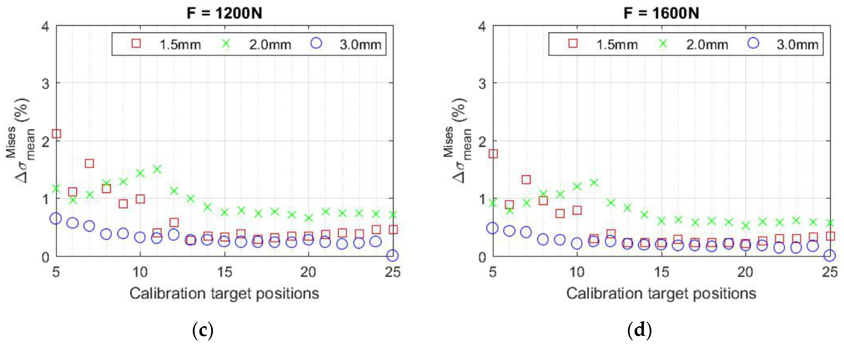
2.1. Experimental Analysis of the Influence of Calibration Parameters on the Results of Strain/Stress Analysis

The reconstruction errors are related to the accuracy of the evaluation of the so-called imaging (calibration) parameters determined in the online calibration procedure integrated into the control software of the correlation system. The Dantec Dynamics correlation systems use a calibration method developed at the turn of the 20th and 21st centuries by Zhang [43,44]. The principle of this method is based on projection geometry (pinhole camera model). It uses a specific technique of recording calibration targets (planar plates with a precisely defined geometry) from different angles of view and rotation to obtain the intrinsic and extrinsic parameters of the cameras. The extrinsic parameters express the transformation from the 3D world to the 3D camera coordinate system. The intrinsic parameters represent the projective transformation from the 3D camera to the 2D image coordinates (Figure 3).

The dependence between the pixel coordinates $\left(x,\hspace{0.17em}y\right)$ of the image and the coordinates $\left(X,\hspace{0.17em}Y,Z\right)$ of the analysed specimen surface points is given by the relation:

$$\left(\begin{array}{c}x\\ y\\ 1\end{array}\right)=K\left[R|t\right]\left(\begin{array}{c}X\\ Y\\ Z\\ 1\end{array}\right),$$

(2)

where the term $K\left[R|t\right]$ expresses the camera’s matrix mapping a 3D world scene into the 2D image plane. The intrinsic camera’s matrix K is defined as follows:

$$K=\left[\begin{array}{ccc}{f}_{\mathrm{x}}& s& c_{\mathrm{x}}\\ 0& f_{\mathrm{y}}& c_{\mathrm{y}}\\ 0& 0& 1\end{array}\right],$$

(3)

where $\left(f_{\mathrm{x}},\hspace{0.17em}{f}_{\mathrm{y}}\right)$ represent the focal lengths (px) of both cameras, s is the distortion coefficient, $\left[c_{\mathrm{x}},\hspace{0.17em}{c}_{\mathrm{y}}\right]$ are the camera’s principal point coordinates (px).

The extrinsic parameters consist of the rotation matrix R and translation vector t. The centre of the camera’s coordinate system is located in its principal point, and the camera’s image plane is defined by its coordinate system axes.

Since the pinhole camera model does not consider lens distortion, to accurately estimate the 3D coordinates of the object surface points using a real camera, the radial α_r and tangential α_t lens distortion parameters must also be determined (Figure 4).

These can then be used to modify the distorted image using relations:

$$\begin{array}{l}{x}_{\mathrm{d}}=x\left[1+k_1\left(x^2+y^2\right)+k_2{\left(x^2+y^2\right)}^2+k_3{\left(x^2+y^2\right)}^3\right],\\ y_{\mathrm{d}}=y\left[1+k_1\left(x^2+y^2\right)+k_2{\left(x^2+y^2\right)}^2+k_3{\left(x^2+y^2\right)}^3\right],\end{array}$$

(4)

where $k_1,\hspace{0.17em}{k}_2,\hspace{0.17em}{k}_3$ are the coefficients of lens radial distortion, or

$$\begin{array}{l}{x}_{\mathrm{d}}=x+\left[2p_{1}xy+p_2\left(3x^2+y^2\right)\right],\\ y_{\mathrm{d}}=y+\left[p_1\left(x^2+3y^2\right)+2p_{2}xy\right],\end{array}$$

(5)

where $p_1,\hspace{0.17em}{p}_2$ are the coefficients of lens tangential distortion. In the case of Dantex Dynamics correlation systems calibration, only $p_1,\hspace{0.17em}{p}_2$ and $k_1,\hspace{0.17em}{k}_2$ coefficients are determined. The $k_3$ coefficient is only used when severe curvatures arise, e.g., in the case of wide/angle lenses.

The calibration of the cameras of the Q-400 Dantec Dynamics correlation system was realised by three different calibration targets with 9 × 9 checkerboard fields. In the first case, each array had an edge length of 1.5 mm (Figure 5a). In this case, the area of the target in the calibration mode, which is performed at the full resolution of the cameras (2452 × 2056 px), covered approximately 12.5% of the field of view. In addition, the authors also performed calibration of the camera system using targets with edge lengths of 2.0 mm (Figure 5b) and 3.0 mm (Figure 5c). The middle of the targets covered approximately 22% of the field of view. The largest covered approximately 50% and almost perfectly copied the evaluated part of the sample. It should be mentioned that the targets with field sizes of 1.5 mm and 3.0 mm were supplied by the manufacturer. They are made by etching in ceramic material with very high precision, guaranteeing a nominal X/Y Standard Deviation of up to 1 μm [45]. In contrast, a 2.0 mm field size target was prepared by authors, printing on a vinyl film applied to a glass plate with an expected standard precision (nominal X/Y standard deviation of up to 150 μm) to analyse the measurement inaccuracies arising in such a case.

During the calibrations of the cameras performed by three different targets, calibration files containing information about the cameras’ intrinsic and extrinsic parameters and the distortion of their lenses, respectively, were sequentially acquired. The first stored file contained the information obtained by evaluating five positions of the calibration target, i.e., the number of positions after which the system estimates for the first time the calibration parameters of the cameras. The last file contained the calibration parameters estimated from 25 different calibration target positions, i.e., the maximum number allowed by the Istra4D V.4.3.0 software. Thus, 21 different calibration files were acquired for each calibration (63 in total) and subsequently used to evaluate the analyses performed.

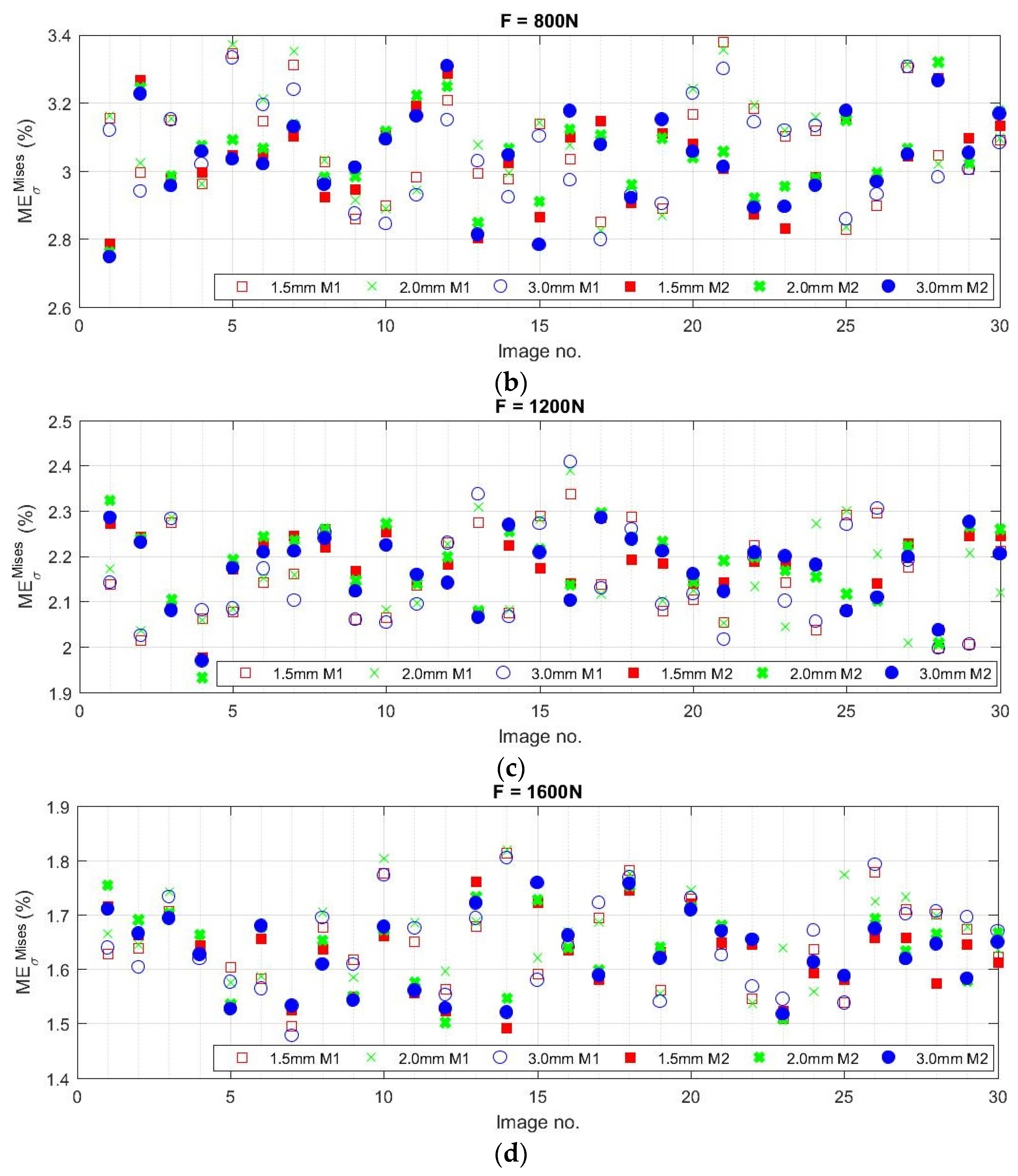
2.2. Experimental Analysis of the Influence of Image Brightness on the Results of Strain/Stress Analysis

The second analysis described in the paper is the analysis of the influence of the image brightness on the results of the strain/stress analyses performed on the above specimen with a hole loaded by tensile loading. For these purposes, 12 measurements were carried out, always realised under different image brightness captured by the stereo DIC system. These were only adjusted by changing the exposure time of the lenses, which can be directly set in the Istra4D V.4.3.0.

A single DLH400DT (Dedolight California, Burbank, USA) light source was used to ensure the illumination of the specimen (see the scheme in Figure 6). The vertical plane (yellow), passing through the light source and the specimen, divides the horizontal plane (red) created by the specimen and the correlation system symmetrically. The mentioned 400 W HMI focusing light head offers a native flood-to-spot range of 50°–4.5° and a focus intensity ratio of 1:20. A dark background was created behind the analysed specimen. The illumination of the specimen was provided by the DL400DHR-NB-400W (Dedolight, USA) lamp with a daylight colour temperature of 5600 K and a maximum lumen of 33,000 lm. The Xenoplan 2.0/28-0901 (Schneider Kreuznach, Bad Kreuznach, Germany) lenses for larger-sized sensors up to 22 mm diagonal were used. These lenses are broadband coated and can be used in the visible range of 400–700 nm or near the infrared of 700–1000 nm. The f-numbers of both lenses were set to F/16.

Selected lighting parameters unchanged during the realised measurements are shown in

Table 1. Selected lighting parameters unchanged during the measurements realised.

Parameter	Value
Adjusted power of the light source	200 W
Distance between the light source and the specimen	1.3 m
Illumination angle of the specimen surface	28°
Adjusted focus angle of the light source	30°
Colour temperature of the lamp	5600 K
F-number of the lenses	F/16
Camera gain	0 dB

. The exposure times were set for each individual measurement, as shown in

Table 2. Exposure times adjusted for the individual measurements.

	Exposure Time		Exposure Time
Measurement 1	0.004 s	Measurement 7	0.022 s
Measurement 2	0.007 s	Measurement 8	0.025 s
Measurement 3	0.01 s	Measurement 9	0.028 s
Measurement 4	0.013 s	Measurement 10	0.031 s
Measurement 5	0.016 s	Measurement 11	0.034 s
Measurement 6	0.019 s	Measurement 12	0.037 s

.

3. Results

3.1. Investigation of the Influence of Calibration Parameters on the Results of Strain/Stress Analysis

The calibration process of the camera(s) of the Dantec Dynamics correlation systems has to be carried out for each measurement separately (either before or after the measurement), while the Istra4D V.4.3.0 program includes a tool providing information about the current accuracy of the obtained calibration parameters. This tool is the so-called calibration residuum, indicating the average inaccuracy of the search for the so-called nodal points of the calibration target. The value of the correlation residuum, together with the cameras’ intrinsic and extrinsic parameters, are displayed in the calibration module of Istra4D from the target’s fourth (and every higher) registered position. These parameters are gradually updated depending on the number of different calibration target positions captured during the calibration of the cameras. The manufacturer claims that eight frames are sufficient for accurate calibration and that the residuum value should not exceed 0.2–0.5 px. Even a small residuum value does not guarantee that the calibration was carried out correctly. However, too large a value (>1.0 px) indicates that some error has occurred in the camera calibration process [46].

Since the standard calibration process runs relatively quickly (takes about 5 min), the user who changes the positions of the calibration target in the field of view of the cameras cannot continuously check the obtained calibration parameters and can only follow the recommendation of the manufacturer of the correlation devices Dantec Dynamics to monitor the value of the calibration residuum. For that reason, this parameter was also registered with each saved calibration file. Figure 7 shows the changes in the calibration residua determined by Istra4D during the three calibration processes. The residuum is the lowest (ca. 0.35–0.45 px) and approximately the same for both calibration targets supplied by Dantec Dynamics (1.5 mm and 3.0 mm) for the entire calibration process. In the case of the 3.0 mm target, a constant trend can be observed from the 10th recorded target position. The calibration residuum is significantly higher in the case of the target manufactured with less precision (2.0 mm). Its value (ca. 0.7 px) exceeds the level of 0.2–0.5 px, which Dantec Dynamics set as the level characterising a correctly performed calibration.

Based on the information presented, the group of calibration targets used is interesting mainly in the following aspects. We have two high-precision calibration targets (1.5 mm and 3.0 mm), where the 3.0 mm target size corresponds approximately to the size of the evaluated part of the specimen (recommended calibration target size), and 1.5 mm is relatively small with respect to the cameras’ field of view in both, calibration and correlation mode. The size of the 2.0 mm target is more suitable than the 1.5 mm target. On the other hand, the accuracy of its manufacture is lower (as confirmed by the obtained data on calibration residua).

The tensile loading measurements described above were performed in correlation mode at an image resolution of 1800 × 1800 px (pixel density approx. 56 px/mm). The reference images with the evaluation area marked are shown in Figure 8. For the evaluation, the facet size was set to 20 × 20 px with an overlap of 5 px.

As the correlation of the images is carried out across facets, it is necessary to smooth the acquired fields for each measurement using the Dantec Dynamics correlation systems. Otherwise, the obtained result is affected by single noise values. Istra4D V.4.3.0 offers two smoothing options. The first one is the ACSP filter for local regression, and the second option is the global Smoothing Spline filter [47]. In our case, a local regression filter with the specified level described in publications [24,41,48] was used to smooth contour and displacement fields.

In the first phase, two variables automatically provided by the Istra4D V4.3.0 software were used as parameters informing about the influence of the calibration parameters on the measurement results. These are the estimated contour statistical error radius (Figure 9) and the deviation of the specimen contour from the best-fit plane (BFP, Figure 10). By analysing the results shown in Figure 9, it was found that the estimated radius of statistical error does not differ significantly when using the high-precision calibration targets supplied by the manufacturer (1.5 mm and 3.0 mm), mainly from the ninth (and each higher) registered position of the calibration target. When using a calibration target manufactured with a lower manufacturing precision (2.0 mm), the estimated error is higher for five up to nine recorded positions and becomes stable from approximately the 12th registered position of the target. It is also interesting to note that the values of the estimated error obtained in this way became slightly smaller after the 11th registered position of the target than those of the original calibration targets. The plots showing the estimated statistical error are of the same character for each loading level. There are no significant changes in their values, which are of the 10⁻¹ μm order.

Based on the analysis of the plots of the deviation of the specimen surface from the best-fit plane (Figure 10), it can be concluded that the plots are also of the same character for each loading level and differ only minimally in values. In the case of using the largest target (3.0 mm), it is possible to observe an approximately constant level for any number of registered positions of the calibration target. Moreover, for this target, the lowest variance of BFP deviation values is observed, and from about the 12th registered position of the target, the values obtained show only slight differences. On the contrary, the most significant variance in values is achieved for a target size of 1.5 mm, which occurs for the number of registered positions of the calibration target less than 12. When using the target with the lowest manufacturing precision (2.0 mm), the variance of the values is not so significant. From its 12th registered position, the BFP deviation reaches a similar level as the other targets.

The causes of the results obtained can be explained from the plots of the cameras’ intrinsic and extrinsic parameters, or lens distortions and their errors, estimated by the Q-400 Dantec Dynamics correlation system automatically during calibration (see Appendix A). Almost all of the plots of the parameters mentioned above obtained using the largest target (3.0 mm) reach a constant level and, simultaneously, the lowest estimated error. When analysing the camera parameters obtained with the smallest target (1.5 mm), the most significant variance of parameters values for the first 12 registered positions can be observed, especially in the case of determining the position of the principal point or the lens distortion coefficients, which harmed the estimation of the deviation from the best-fit plane when evaluated using the calibration files from the first half of the calibration process. The authors attribute this phenomenon to the target size, which covers only approximately 12.5% of the cameras’ field of view used in calibration mode. Thus the correlation system needs to acquire and evaluate a larger number of its different positions to determine these parameters correctly. However, from the 12th registered position, the plots take on a constant character with low estimated errors and approach those obtained with the largest (3.0 mm) calibration target. When using a middle (2.0 mm) target, the lower precision of its manufacture was reflected in the fact that, in some cases, the camera parameters started to stabilise later (from about the 15th recorded position of the target) or did not stabilise at all. In addition, several estimated parameters differed significantly from those obtained with the original calibration targets with a higher guaranteed manufacturing accuracy. Also, the correlation system estimated the largest errors in calibration parameters assessment when the 2.0 mm target was used.

From the above plots of calibration residua, camera parameters, or lens distortions, it is possible to predict which correlation system calibration should provide the most accurate (and, conversely, the least accurate) results. However, from the mechanics of materials point of view, it is more important to know what effect changing these parameters will have on the results of the strain/strain analyses. Therefore, in the second phase, an analysis was carried out in which the values of the equivalent stresses according to von Mises theory were compared in a full-field manner. The comparison was carried out for four specimen loading levels (F = 400 N, F = 800 N, F = 1200 N, and F = 1600 N), the same as in the previous analysis, always taking as reference the field determined using the calibration file obtained by calibrating the largest (3.0 mm) target at the maximum number of registered positions. The mean values of the relative differences of the equivalent stresses $\Delta {\sigma }_{\mathrm{mean}}^{\mathrm{Mises}}$ were obtained based on the relation:

$$\Delta {\sigma }_{\mathrm{mean}}^{\mathrm{Mises}}=\mathrm{mean}\left(\left|\frac{{\sigma }_{\mathrm{i}}^{\mathrm{Mises}}\left(a,b\right)-{\sigma }_{\mathrm{ref}.}^{\mathrm{Mises}}\left(a,b\right)}{{\sigma }_{\mathrm{ref}.}^{\mathrm{Mises}}\left(a,b\right)}\right|\right)\cdot 100\%$$

(6)

where $\left(a,b\right)$ represent the facet centres coordinates of the reconstructed specimen surface, ${\sigma }_{\mathrm{i}}^{\mathrm{Mises}}$ is the equivalent von Mises stress determined for the i^th position of the calibration target, ${\sigma }_{\mathrm{ref}.}^{\mathrm{Mises}}$ is the reference equivalent von Mises stress determined using the calibration file obtained by calibrating the largest (3.0 mm) target at the maximum number of registered positions. The MOSTRAN V.1.0 program, developed in MATLAB at the authors’ workplace, was used to obtain the equivalent von Mises stress fields.

The plots of the mean relative differences in the evaluated equivalent von Mises stresses can be seen in Figure 11. Suppose we disregard the results obtained in calibration with the number of registered calibration target positions less than 8 (which, according to [37], is the minimum at which accurate results should be obtained). In that case, the most significant differences are obtained using the middle (2.0 mm) target with a lower manufacturing precision. However, the percentage differences obtained when using the smallest (1.5 mm) target reach more significant levels for fewer recorded positions, which is again related to the estimation of the calibration parameters. From the 13th recorded position of the calibration targets, the results obtained when using the original targets (1.5 mm and 3.0 mm) differ only minimally.

As the number of recorded calibration target positions increases, it is possible to observe a decreasing character of the relative differences value obtained in the evaluated equivalent von Mises stresses. The achieved levels of differences evaluated for a higher number (at least 13) of calibration target positions do not exceed the value of 2% for all four evaluated measurements.

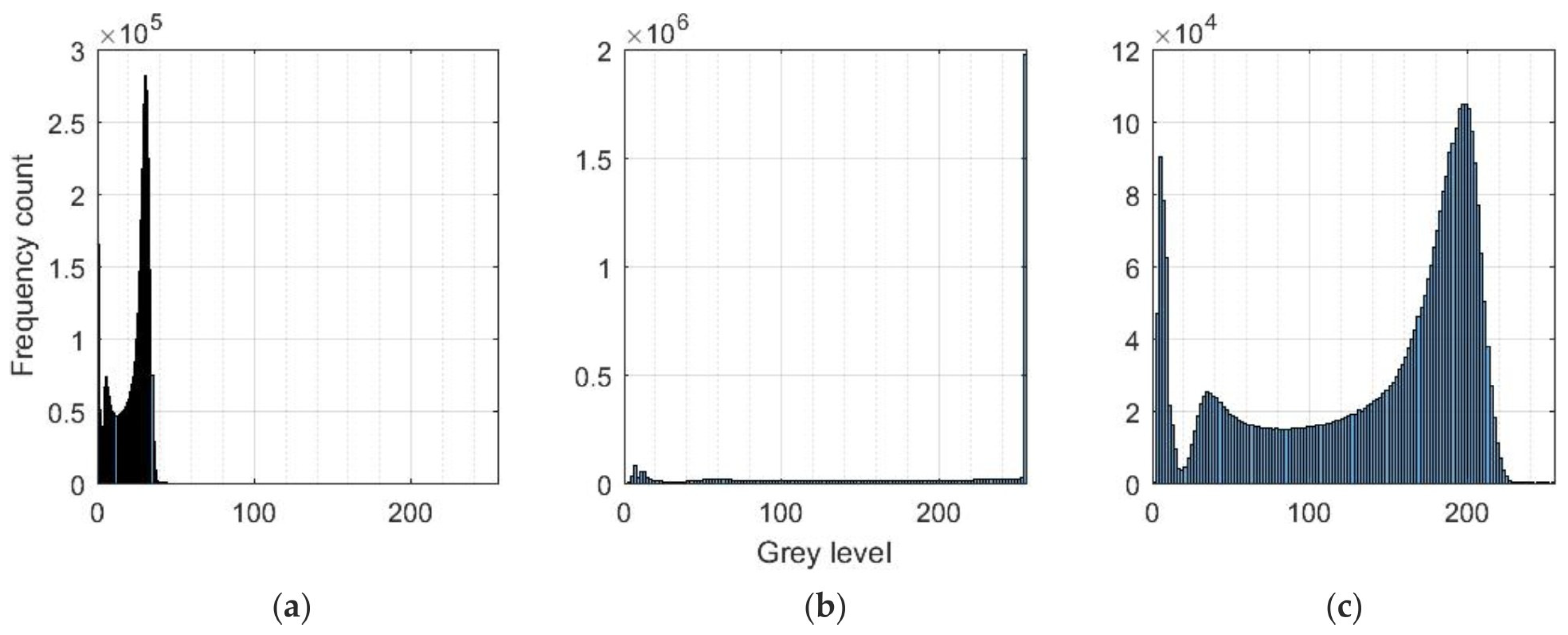
3.2. Investigation of the Influence of Image Brightness on the Results of Strain/Stress Analysis

All of the reference images acquired during the 12 measurements mentioned in Section 2.2 can be seen in Figure 12. All these images were exported to MATLAB R2020a (MathWorks, Natick, MA, USA), where they were processed to evaluate their mean grey values (MGV). The obtained information about MGV characterising the image brightness is written in the lower right part of the captured images shown in Figure 12. A similar procedure to the calibration influence analysis was established, i.e., the mean relative differences in the evaluated equivalent von Mises stresses were determined to assess the influence of the changing image brightness.

As a reference for comparing the results, a field of equivalent von Mises stress was chosen, obtained from the images of the seventh measurement, with a determined MGV = 122, which approximately corresponds to the middle intensity of the evaluated images. The analysis of the differences in the fields mentioned above due to the change of the image brightness was carried out using all the calibration files obtained during the calibration process of the correlation system cameras with 1.5 mm, 2.0 mm, and 3.0 mm targets, resulting in the 3D plots shown in Figure 13.

Based on the analysis of the 3D plots shown in Figure 13, it can be concluded that there is a relatively wide range of mean gray values (approximately from 56 to 171) without significant differences in the evaluated equivalent von Mises stresses. The values of the relative differences in the compared fields of the equivalent von Mises stress for images acquired within the range of mean gray values from 56 to 171 are given in

Table 3. Mean relative differences in the evaluated equivalent von Mises stresses obtained by varying the image intensity over a range of mean gray values from 56 to 171.

	F = 400 N	F = 800 N	F = 1200 N	F = 1600 N
$\Delta {\sigma }_{\mathrm{mean}}^{\mathrm{Mises}}\hspace{0.17em}(\%)$	from 6.8 up to 7.5	from 3.1 up to 3.6	from 2.1 up to 2.6	from 1.6 up to 1.9

. The change occurs when the image is too bright (overexposed) with a mean gray value greater than 171. There is also an increase in the deviation for images with a low mean gray value (less than 56). Moreover, the evaluation becomes problematic when the images are too dark (less than 22) or too bright (more than 194) because there are problems with finding the so-called starting points, i.e., the places where the algorithm starts to compare the images.

The deviations due to the use of different calibration sets (varying CTP) reach approximately the same levels as for the measurement described above (up to a maximum of 3% within all measurements). However, the levels of $\Delta {\sigma }_{\mathrm{mean}}^{\mathrm{Mises}}$ observed for the 12 measurements performed at varying image brightness were significantly larger than those obtained when comparing results from a single measurement. The following analysis was performed to reveal the reason causing the higher differences in equivalent von Mises stresses. For each of the four loading levels, i.e., for F = 400 N up to F = 1600 N, two measurements were performed, during which 30 images of the loaded specimen were captured under the same measurement conditions (MGV = 122). From the evaluated data, the mean relative measurement error was then determined according to the relation:

$$M{E}_{\sigma }^{\mathrm{Mises}}=\mathrm{mean}\left(\left|\frac{{\sigma }_{\mathrm{i}}^{\mathrm{Mises}}\left(a,b\right)-{\sigma }_{\mathrm{mean}}^{\mathrm{Mises}}\left(a,b\right)}{{\sigma }_{\mathrm{mean}}^{\mathrm{Mises}}\left(a,b\right)}\right|\right)\cdot 100\%$$

(7)

where i = 1, 2, 3, ..., 30 represents the image number, ${\sigma }_{\mathrm{mean}}^{\mathrm{Mises}}\left(a,b\right)$ is an average value of the equivalent von Mises stress evaluated in the facet centre with coordinates $\left(a,b\right)$ calculated from all the 30 images. The obtained levels of individual measurement errors are shown in Figure 14. The mean relative measurement error values evaluated from the set of 60 images (30 and 30 from each measurement) for each load level and their standard deviations are shown in

Table 4. Mean relative measurement errors and their standard deviations obtained for individual load levels.

Tensile Force	Mean Relative Measurement Errors and Their Standard Deviations (%)
	Calibration target 1.5 mm	Calibration target 2.0 mm	Calibration target 3.0 mm
F = 400 N	6.65 ± 0.31	6.70 ± 0.33	6.66 ± 0.32
F = 800 N	3.05 ± 0.14	3.07 ± 0.14	3.04 ± 0.14
F = 1200 N	2.17 ± 0.10	2.17 ± 0.09	2.16 ± 0.09
F = 1600 N	1.63 ± 0.08	1.65 ± 0.08	1.64 ± 0.08

.

Based on the analysis of the obtained results, it can be concluded that the mean differences in the equivalent von Mises stress values achieved when the intensity of the images is changed from the mean grey value of 56 up to 171 only slightly exceed the levels of the evaluated measurement errors. Thus, within the range indicated, there is no significant influence on the results of the realised stress analyses.

4. Discussion

This paper describes the influence of calibration parameters and image brightness established when strain/stress analyses are carried out on a small area of a planar specimen with a hole using stereoscopic low-speed digital image correlation. The experiments aimed to obtain this information to improve the accuracy of the results of the analyses related to the quantification of residual stresses by means of the hole-drilling method combined with DIC, which has recently received increased attention. By such measurements, it is possible to obtain relatively quickly and efficiently information on the strains relieved during the formation of the hole or groove in the analysed specimen, which is the principle for determining the residual stresses by the mentioned semi-destructive approaches. In addition, the measurement is easily repeatable, which leads to at least a saving of time related to the preparation of the strain gauge measurement. However, the disadvantages of DIC over conventional methods of measuring the strains relieved are:

• the problem of applying a standard digital image correlation system with commercially available drilling equipment;
• the lower sensitivity of the cameras compared to specialised strain gauge rosettes.

Problems associated with the application of digital image correlation systems with commercially supplied drilling equipment (e.g., the body of the drilling equipment not being adapted to the application of optical methods, the principle of which is to acquire the surface of the analysed object repeatedly) are often overcome by the installation of the optical system at greater distances, or by the development of custom drilling/imaging equipment. However, the lower sensitivity of correlation system cameras compared to strain gauge rosettes is guaranteed to lead to some measurement inaccuracy. However, to avoid further adverse effects, it is essential to be aware of all possible aspects that could adversely affect the results of strain/stress analyses performed by correlation systems.

The paper describes several analyses processed in MATLAB or MOSTRAN V.1.0 program, developed at the authors’ workplace. Based on the obtained results, it can be concluded that the size of the calibration target, the accuracy of its manufacture, as well as the number of its registered positions in the process of calibration of the stereo-camera DIC system can affect the results of strain/stress analyses. To minimize their influence, the authors of the paper suggest:

• if possible, use calibration targets whose size corresponds approximately to the field of view of the cameras used in correlation mode;
• if the calibration target used is significantly smaller than the field of view of the cameras, there is a risk that some of the calibration parameters will not be estimated correctly if the number of registered target positions is less than 10; it is, therefore, recommended to register as many different positions of the target chosen for calibrating the cameras as possible (minimum 15);
• a target with a lower manufacturing accuracy should be used for the calibration of the cameras only in case of necessity—however—it has to be taken into account that the measurement results will be obtained with a higher measurement uncertainty than in the case of targets manufactured with a guaranteed higher manufacturing accuracy.

The determination of appropriate image brightness is another factor that can influence the results of strain/stress analyses performed by DIC. The performed measurements show that as long as the surface of the analysed specimen is illuminated uniformly and the lighting conditions are unchanged throughout the experimental period, there is a relatively wide range of image brightness (expressed by the mean grey value MGV from 56 up to 171) at which a nearly constant relative difference in the compared von Mises stresses is achieved for each loading level. Subsequent analysis has shown that the levels of these differences only slightly exceed the mean relative measurement errors evaluated on the analysed region of the specimen with the hole. On the contrary, images acquired with smaller or larger MGV cause significant differences in the obtained results or do not allow for evaluation of the realised measurement at all. The reasons can be found in that the darkest and brightest images thus obtained are either represented by a narrow range of intensity values (Figure 15a) or a significant representation of one of the intensities (Figure 15b). Figure 15c shows the intensity histogram obtained for images with MGV = 122 and significantly better intensity distribution of individual image points.

The classification of image quality into five categories, i.e., unsuitable too dark images, underexposed images, suitable image brightness, overexposed images, and unsuitable too bright images, determined from the analysis of the differences in the evaluated equivalent stress fields, is shown in

Table 5. Classification of images quality based on their mean grey value (MGV).

Image Quality	MGV	Consequence
unsuitable too dark images	less than 22	measurement evaluation issues
underexposed images	from 22 up to 55	increase in deviation in the evaluated stresses
suitable image brightness	from 56 up to 171	deviation in the evaluated stresses approximately at the measurement error level
overexposed images	from 172 up to 194	increase in deviation in the evaluated stresses
unsuitable too bright images	more than 194	measurement evaluation issues

.

5. Conclusions

The accuracy of the digital image correlation method depends on many factors. In this paper, it was shown that the results of strain/stress analyses performed on small areas (approx. 25 × 25 mm) of a specimen with a hole by a stereo-camera DIC system are influenced by the appropriate choice of the calibration target and the correct adjustment of the brightness of the images. Based on the presented results, the authors recommend choosing a calibration target with guaranteed high production accuracy, sized to cover the cameras’ field of view in the correlation mode. The lowest influence on the results occurs when the largest possible number of different positions of the calibration target are registered. It is recommended that the brightness of the images should be set so that the mean grey value is in a range from 56 up to 171, with the intensity values of the individual image points as evenly distributed as possible.

References

1. Lecompte, D.; Smits, A.; Bossuyt, S.; Sol, H.; Vantomme, J.; Van Hemelrijck, D.; Habraken, A.M. Quality assessment of speckle patterns for digital image correlation. Opt. Laser Eng. 2006, 44, 1132–1145. [Google Scholar] [CrossRef]
2. Pan, B.; Qian, K.; Xie, H.; Asundi, A. On errors of digital image correlation due to speckle patterns. In Proceedings of the International Conference on Experimental Mechnics 2008 and Seventh Asian Conference on Experimental Mechanics, Nanjing, China, 8–11 November 2008. [Google Scholar]
3. Hua, T.; Xie, H.; Wang, S.; Hu, Z.; Chen, P.; Zhang, Q. Evaluation of the quality of a speckle pattern in the digital image correlation method by mean subset fluctuation. Opt. Laser Technol. 2011, 43, 9–13. [Google Scholar] [CrossRef]
4. Haddadi, H.; Belhabib, S. Use of rigid-body motion for the investigation and estimation of the measurement errors related to digital image correlation technique. Opt. Laser Eng. 2008, 46, 185–196. [Google Scholar] [CrossRef]
5. Barranger, Y.; Doumalin, P.; Dupré, J.C.; Germaneau, A. Digital Image Correlation accuracy: Influence of kind of speckle and recording setup. EPJ Web Conf. 2010, 6, 31002. [Google Scholar] [CrossRef]
6. Crammond, G.; Boyd, S.W.; Dulieu-Barton, J.M. Speckle pattern quality assessment for digital image correlation. Opt. Laser Eng. 2013, 51, 1368–1378. [Google Scholar] [CrossRef]
7. Kammers, A.D.; Daly, S. Small-scale patterning methods for digital image correlation under scanning electron microscopy. Meas. Sci. Technol. 2011, 22, 125501. [Google Scholar] [CrossRef]
8. Cannon, A.H.; Hochhalter, J.D.; Mello, A.W.; Bomarito, G.F.; Sangid, M.D. Microstamping for improved speckle patterns to enable digital image correlation. Microsc. Microanal. 2015, 21, 451–452. [Google Scholar] [CrossRef]
9. Bossuyt, S. Optimized patterns for digital image correlation. In Proceedings of the 2012 Annual Conference on Experimental and Applied Mechanics, Volume 3: Imaging Methods for Novel Materials and Challenging Applications, Costa Mesa, CA, USA, 11–14 June 2012. [Google Scholar]
10. Bomarito, G.F.; Hochhalter, J.D.; Ruggles, T.J.; Cannon, A.H. Increasing accuracy and precision of digital image correlation through pattern optimization. Opt. Laser Eng. 2017, 91, 73–85. [Google Scholar] [CrossRef]
11. Song, J.; Zang, J.; Liu, F.; Lu, K. Quality assessment of laser speckle patterns for digital image correlation by a Multi-Factor Fusion Index. Opt. Laser Eng. 2020, 124, 105822. [Google Scholar] [CrossRef]
12. Zhang, C.; Liu, C.; Xu, Z. High-Accuracy Three-Dimensional Deformation Measurement System Based on Fringe Projection and Speckle Correlation. Sensors 2023, 23, 680. [Google Scholar] [CrossRef]
13. Souto Janeiro, A.; Fernández López, A.; Chimeno Manguan, M.; Pérez-Merino, P. Three-Dimensional Digital Image Correlation Based on Speckle Pattern Projection for Non-Invasive Vibrational Analysis. Sensors 2022, 22, 9766. [Google Scholar] [CrossRef]
14. Craig, W.D.; Leeuwen, F.B.; Jarrett, S.R.; Hansen, R.S.; Berke, R.B. Using text as a native speckle pattern in digital image correlation. J. Strain Anal. Eng. Des. 2022, 57, 539–555. [Google Scholar] [CrossRef]
15. Hu, X.; Xie, Z.; Liu, F. Assessment of speckle pattern quality in digital image correlation from the perspective of mean bias error. Measurement 2021, 173, 108618. [Google Scholar] [CrossRef]
16. Sun, Y.; Pang, J.H. Study of optimal subset size in digital image correlation of speckle pattern images. Opt. Lasers Eng. 2007, 45, 967–974. [Google Scholar]
17. Pan, B.; Xie, H.; Wang, Z.; Qian, K.; Wang, Z. Study on subset size selection in digital image correlation for speckle patterns. Opt. Express 2008, 16, 7037–7048. [Google Scholar] [CrossRef]
18. Lane, C.; Burguete, R.L.; Shterenlikht, A. An objective criterion for the selection of an optimum dic pattern and subset size. In Proceedings of the XIth International Congress and Exposition on Experimental and Applied Mechanics, Orlando, FL, USA, 2–5 June 2008. [Google Scholar]
19. Wang, M.; Cen, Y.; Hu, X.; Yu, X.; Xie, N.; Wu, Y.; Xu, P.; Xu, D. A weighting window applied to the digital image correlation method. Opt. Laser Technol. 2009, 41, 154–158. [Google Scholar] [CrossRef]
20. Huang, J.; Pan, X.; Peng, X.; Yuan, Y.; Xiong, C.; Fang, J.; Yuan, F. Digital image correlation with self-adaptive Gaussian windows. Exp. Mech. 2013, 53, 505–512. [Google Scholar] [CrossRef]
21. Li, B.J.; Wang, Q.; Duan, D.P.; Chen, J.A. Modified digital image correlation for balancing the influence of subset size choice. Opt. Eng. 2017, 56, 054104. [Google Scholar] [CrossRef]
22. Wang, X.; Liu, X.; Zhu, H.; Ma, S. Spatial-temporal subset based digital image correlation considering the temporal continuity of deformation. Opt. Laser Eng. 2017, 90, 247–253. [Google Scholar] [CrossRef]
23. Xing, T.; Zhu, H.; Wang, L.; Liu, G.; Ma, Q.; Wang, X.; Ma, S. High accuracy measurement of heterogeneous deformation field using spatial-temporal subset digital image correlation. Measurement 2020, 156, 107605. [Google Scholar] [CrossRef]
24. Hagara, M.; Bocko, J. The aspects of stress analysis performed by digital image correlation method related with smoothing and its influence on the results. Acta Mechatron. 2018, 3, 15–21. [Google Scholar] [CrossRef]
25. Peng, B.; Zhang, Q.; Zhou, W.; Hao, X.; Ding, L. Modified correlation criterion for digital image correlation considering the effect of lighting variations in deformation measurements. Opt. Eng. 2012, 51, 017004. [Google Scholar] [CrossRef]
26. Pan, B.; Wu, D.; Xia, Y. An active imaging digital image correlation method for deformation measurement insensitive to ambient light. Opt. Laser Technol. 2012, 44, 204–209. [Google Scholar] [CrossRef]
27. Poncelet, M.; Leclerc, H. A Digital Image Correlation algorithm with light reflection compensation. Exp. Mech. 2015, 55, 1317–1327. [Google Scholar] [CrossRef]
28. Simončič, S.; Podržaj, P. An improved digital image correlation calculation in the case of substantial lighting variation. Exp. Mech. 2017, 57, 743–753. [Google Scholar] [CrossRef]
29. Zhao, J.; Yang, P.; Zhao, Y. Neighborhood binary speckle pattern for deformation measurements insensitive to local illumination variation by digital image correlation. Appl. Opt. 2017, 56, 4708–4719. [Google Scholar] [CrossRef]
30. Li, B.J.; Wang, Q.B.; Duan, D.P.; Chen, J.A. Using grey intensity adjustment strategy to enhance the measurement accuracy of digital image correlation considering the effect of intensity saturation. Opt. Lasers Eng. 2018, 104, 173–180. [Google Scholar] [CrossRef]
31. Hu, X.; Xie, Z.; Liu, F. Estimating gray intensities for saturated speckle to improve the measurement accuracy of digital image correlation. Opt. Laser Eng. 2021, 139, 106510. [Google Scholar] [CrossRef]
32. ASTM E837-13a; Standard Test Method for Determining Residual Stresses by the Hole-Drilling Strain-Gage Method. American Society for Testing and Materials: West Conshohocken, PA, USA, 2013.
33. Rendler, N.J.; Vigness, I. Hole-drilling strain-gage method of measuring residual stresses. Exp. Mech. 1966, 6, 577–586. [Google Scholar] [CrossRef]
34. Schajer, G.S. Application of finite element calculations to residual stress measurements. J. Eng. Mater. Technol. 1981, 103, 157–163. [Google Scholar] [CrossRef]
35. Schajer, G.S. Measurement of non-uniform residual stress using the hole-drilling method: Part II-Practical application of the integral method. J. Eng. Mater. Technol. 1988, 110, 344–349. [Google Scholar] [CrossRef]
36. Schajer, G.S.; Tootonian, M. A new rosette design for more reliable hole-drilling residual stress measurements. Exp. Mech. 1997, 37, 299–306. [Google Scholar] [CrossRef]
37. Schajer, G.S.; Whitehead, P.S. Hole-Drilling Method for Measuring Residual Stresses, 1st ed.; Springer Nature Switzerland AG: Cham, Switzerland, 2018; pp. 1–186. [Google Scholar]
38. Viotti, M.R.; Dolinko, A.E.; Galizzi, G.E.; Kaufmann, G.H. A portable digital speckle pattern interferometry device to measure residual stresses using the hole drilling technique. Opt. Lasers Eng. 2006, 44, 1052–1066. [Google Scholar] [CrossRef]
39. Brynk, T.; Romelczyk-Baishya, B. Residual stress estimation based on 3D DIC displacement filed measurement around drilled holes. Procedia Struct. Integr. 2018, 13, 1267–1272. [Google Scholar] [CrossRef]
40. Pástor, M.; Hagara, M.; Virgala, I.; Kaľavský, A.; Sapietová, A.; Hagarová, L. Design of a Unique Device for Residual Stresses Quantification by the Drilling Method Combining the PhotoStress and Digital Image Correlation. Materials 2021, 14, 314. [Google Scholar] [CrossRef]
41. Hagara, M.; Trebuňa, F.; Pástor, M.; Huňady, R.; Lengvarský, P. Analysis of the aspects of residual stresses quantification performed by 3D DIC combined with standardized hole-drilling method. Measurement 2019, 137, 238–256. [Google Scholar] [CrossRef]
42. Hagara, M.; Pástor, M. A Complex Review of the Possibilities of Residual Stress Analysis Using Moving 2D and 3D Digital Image Correlation System. J. Mech. Eng. 2021, 71, 61–78. [Google Scholar]
43. Zhang, Z. A Flexible New Technique for Camera Calibration; Microsoft Research Technical Report MSR-TR-98-71; Microsoft: Redmond, WA, USA, 1998. [Google Scholar]
44. Zhang, Z. Flexible Camera Calibration by Viewing a Plane from Unknown Orientations. In Proceedings of the 7th IEEE International Conference on Computer Vision, Kerkyra, Greece, 20–27 September 1999. [Google Scholar]
45. Dantec Dynamics. Calibration Targets (DIC): High-Precision DIC Reference Measurement Objects; Data Sheet 0752_v3; Dantec Dynamics: Skovlunde, Denmark, 2022. [Google Scholar]
46. Dantec Dynamics. Q-400 User Manual; Dantec Dynamics: Skovlunde, Denmark, 2012. [Google Scholar]
47. Dantec Dynamics. Influence of Filter Parameter on Q-4xx Measurement Results; Technical Note; Dantec Dynamics: Skovlunde, Denmark, 2013. [Google Scholar]
48. Hagara, M.; Pástor, M.; Delyová, I. Set-up of the Standard 2D-DIC System for Quantification of Residual Stresses. In Proceedings of the EAN 2019—57th Conference on Experimental Stress Analysis, Luhačovice, Czech Republic, 3–6 June 2019. [Google Scholar]
Figure 1. Dimensions (mm) and shape of the specimen with the cameras’ field of view marked.
Applsci 13 09512 g001
Figure 2. Transformation parameters used in the algorithm based on pseudo-affine transformation.
Applsci 13 09512 g002
Figure 3. A transformation from the 3D world coordinates of the analysed object to the 2D pixel coordinates of the image.
Applsci 13 09512 g003
Figure 4. Effect of radial and tangential distortion on the position of the registered surface point.
Applsci 13 09512 g004
Figure 5. Targets used for camera calibration and comparison of their sizes to the field of view (1800 × 1800 px) set in the correlation mode: (a) 1.5 mm, (b) 2.0 mm, (c) 3.0 mm.
Applsci 13 09512 g005
Figure 6. The layout of the light source and the DIC system with respect to the analysed object with the dark background created.
Applsci 13 09512 g006
Figure 7. Plot of calibration residua obtained when calibrating the correlation system using three different calibration targets.
Applsci 13 09512 g007
Figure 8. Captured reference images with marked evaluation area.
Applsci 13 09512 g008
Figure 9. Plots of the estimated contour statistical error radius: (a) F = 400 N, (b) F = 800 N, (c) F = 1200 N, (d) F = 1600 N.
Applsci 13 09512 g009
Figure 10. Plots of the specimen surface deviation from the best-fit plane: (a) F = 400 N, (b) F = 800 N, (c) F = 1200 N, (d) F = 1600 N.
Applsci 13 09512 g010
Figure 11. Influence of the estimated calibration parameters on the evaluated equivalent von Mises stresses: (a) F = 400 N, (b) F = 800 N, (c) F = 1200 N, (d) F = 1600 N.
Applsci 13 09512 g011aApplsci 13 09512 g011b
Figure 12. Images of the analysed specimen acquired under changing exposure time of the lenses subjected to analysis of the effect of image brightness on the strain/stress analysis results. Note: MGV is indicated in the lower right corner of each image.
Applsci 13 09512 g012
Figure 13. Influence of the image brightness and estimated calibration parameters on the evaluated equivalent von Mises stress: (a) F = 400 N, (b) F = 800 N, (c) F = 1200 N, (d) F = 1600 N. Note: MGV (mean gray value), CTP (calibration target positions).
Applsci 13 09512 g013
Figure 14. Mean relative measurement errors for the analysis of equivalent von Mises stress obtained around the specimen hole for different load levels: (a) F = 400 N, (b) F = 800 N, (c) F = 1200 N, (d) F = 1600 N. Note: M1—measurement 1, M2—measurement 2.
Applsci 13 09512 g014aApplsci 13 09512 g014b
Figure 15. The intensity histograms obtained for: (a) darkest image (MGV = 22), (b) brightest image (MGV = 194), (c) image with MGV = 122. Note: 0 corresponds to a black colour, 255 corresponds to a white colour.
Applsci 13 09512 g015