Advanced Bayesian Network for Task Effort Estimation in Agile Software Development

Abstract

Effort estimation is always quite a challenge, especially for agile software development projects. This paper describes the process of building a Bayesian network model for effort prediction in agile development. Very few studies have addressed the application of Bayesian networks to assess agile development efforts. Some research has not been validated in practice, and some has been validated on one or two projects. This paper aims to bring the implementation and use of Bayesian networks for effort prediction closer to the practitioners. This process consists of two phases. The Bayesian network model for task effort estimation is constructed and validated in the first phase on real agile projects. A relatively small model showed satisfactory estimation accuracy, but only five output intervals were used. The model was proven to be useful in daily work, but the project manager wanted to obtain more output intervals, although increasing the number of output intervals reduces the prediction accuracy. In the second phase, the focus is on increasing the number of output intervals while maintaining satisfactory accuracy. The advanced model for task effort estimation is developed and tested on real projects of two software firms.

1. Introduction

Inaccurate estimates of time and cost have the greatest impact on the failure of software projects [1,2]. Traditional software project prediction models are either unreliable or require sophisticated metrics to be rendered reliable [3], thus representing a problem in agile software development (ASD). Many metrics used in traditional software development project planning simply cannot be used in agile development project planning. In recent years, most studies on predicting effort in ASD have been based on machine learning techniques [4,5,6,7]. Some studies show that traditional estimation methods can be successfully replaced by Artificial Intelligence (AI) [7,8,9].

The typical problems of traditional effort, cost, and quality prediction models can be overcome by using Bayesian Network (BN) models [10,11], due to the following:

• Flexibility of the BN building process (based purely on expert judgment, empirical data, or the combination of both),
• Ability to reflect causal relationships,
• Explicit incorporation of uncertainty as a probability distribution for each variable,
• Graphical representation that makes the model clear,
• Ability of both, forward and backward inferences,
• Ability to run the model with missing data.

The prediction accuracy can be significantly increased by using empirical data [12,13,14]. There is a gap between theory and practice. Although the number of studies on the application of intelligent techniques in agile software development is increased, less than 50% of these studies have been applied in practice [4]. Therefore, the purpose of this article is to increase the understanding of practitioners and facilitate BN implementation.

In theory and practice, companies mainly measure and estimate software development functionality, effort, time and cost [15,16,17,18]. Companies using agile methodologies are constantly making tradeoff decisions between functionality and effort, cost, and time [15]. Such a tradeoff is sometimes made in academic literature also—the terms ‘cost’ and ‘effort’ are used interchangeably in the systematic review of software development cost estimation [19].

This is especially important in micro and small companies. Consequently, data from real agile projects are used for building this BN model. The model is intended for the prediction of smaller parts of projects (project tasks) and not for their scheduling. For that reason, the terms ‘effort’ and ‘time’ are used interchangeably in this paper. For a measurement unit, we use time-based units (man-hour), as many companies use [20].

In the first phase [21], a BN model (old BN model) with eighteen nodes was developed. Empirical data were used for thirteen nodes, while values were calculated for five nodes. This BN model showed an estimation accuracy greater than 90%, but its outcomes are probability distributions for only five intervals. This decreases the prediction precision because all the values in an interval are treated equally. For example, values 45 and 61 from the interval ‘>40.1 h’ have the same probabilities.

Although the developed BN model is not overly complex, the objectives of the second phase are to further simplify the BN model and to increase the output interval number, without affecting the accuracy of the prediction.

The authors wanted to further simplify the model, reduce the number of input parameters, as well as increase the number of output intervals without reducing the model’s estimation accuracy.

Therefore, the rest of this paper is structured as follows: an investigation of current usages of BN models for software effort prediction (Section 2); a description of their detailed building processes and the validation of the proposed BN model (Section 3); the explanation of the application of the respective BN model in another company (Section 4); and the presentation of conclusions and the outlines of future work (Section 5).

2. Related Works

In recent years, the application of methods based on Artificial Intelligence (AI) in Software Effort Estimation (SEE) has increased [22,23].

In 2017, Dragicevic et al. [21] conducted a literature search on the use of Bayesian networks for effort estimation in agile software development projects. This search has resulted in a small number of papers.

A search for new literature resulted in several new papers. Perkusich et al. [24] presented an improved version of their BN model for assessing the quality of the software process in Scrum projects. A comparison of old and improved versions, for ten different scenarios, proved the improvement in the model, so that the BN model adequately represented Scrum projects from the Scrum masters’ point of view. The model was built according to an agile approach and can be adapted to any Scrum team.

Radu [25] proposed a BN model for effort prediction in agile projects. Based on the literature, twenty-one influencing factors were identified and classified into two main categories. The relationships between those factors were determined based on discussions with developers and literature searches. The model has not been validated.

Several studies have used BN models to evaluate user stories in a Scrum context. Malgonde and Chari [26] developed a model to predict the user story realization effort. Seven machine learning algorithms, including BN, were applied to a database with 503 user stories. None of these algorithms consistently outperformed the others, so the authors developed an ensemble-based algorithm, resulting in better prediction. The algorithm was validated on two projects’ data from a database. Durán et al. [27] proposed a BN model whose nodes represented factors for assessing the complexity of a user story. The weight factors of the edges were determined based on the experts’ judgment. The model was intended for the use of inexperienced teams to help them estimate the required effort more easily. Another BN model was used to predict the user story’s effort [28]. That model was based on narrative texts. Further on, a BN model proposed by [29] could be useful for helping novice developers to estimate the user story’s complexity. Although Planning Poker is a commonly used estimation technique in Scrum projects, for novice developers, it is not an easy task to estimate a user story’s complexity and importance, so the BN model could be used instead.

The sizes of the mentioned BN models vary: some are relatively large [24,25], while others are relatively small [30,31]. Dynamic BN models are usually smaller, but they are unable to predict effort in the first iteration. The practical application of BN models in effort estimation is a motivation for this research, so the target is to create a model that has a satisfactory accuracy with a small set of input data and that can be used as early as possible (including project’s first iteration). Respectable literature shows that early estimates range from 60% to 160% [15], or even from 25% to 400% [18] of the final result.

To summarize, the existing BN models do not estimate task effort. In addition, none of the above described models meet all the following requirements:

• Suitability for agile development, regardless of used agile methods and/or practices.
• Minimal set of input parameters, provided that the method predicts with at least 75% accuracy.
• Possibility of using the BN model at the start of the project.
• Validation based on larger sample size (not just a few samples).

The above discussion shows that a small number of studies explore the use of Bayesian networks for effort estimation in agile projects, and that the results of most of these studies have not been validated in practice.

3. The BN Model

The BN is a graphical model that describes probabilistic relationships between causally related variables.

The BN is formally determined by the pair BN = (G, P), where G is a directed acyclic graph (DAG), and P is a set of local probability distributions for all the variables in the network. A directed acyclic graph G = (V (G), E (G)) consists of a finite, nonempty set of tuples V (G) = {(s₁, V₁), (s₂, V₂), …, (s_n, V_n)} and a finite set of directed edges E (G) ⊆ V (G) × V (G). Nodes V₁, V₂, …, Vn correspond to random variables X = (X₁, …, X_n), which can take on a certain set of values s_i (depending on the problem being modelled). The terms variable and node will be used interchangeably in this paper. The edges E (G) = {e_i,_j} represent dependencies among variables. A directed edge e_i,_j from V_i to V_j for V_i, V_j ∈ V(G) shows that V_i (parent node) is a direct cause of V_j (child node).

Each variable X_i has a joint probability distribution P (X_i|parent (X_i)), which shows the impact of a parent on a child. If X_i has no parents, its probability distribution is unconditional, otherwise, it is conditional. The probability distribution of variables in a BN must satisfy the Markov condition, which states that each variable X_i is independent of its nondescendents, given its parents in G [32]. The BN decomposes the joint probability distribution P (X₁, …, X_n) into a product of conditional probability distributions for each variable, given its parents in the following:

$$\mathrm{P}\left({\mathrm{x}}_1,\dots ,{\mathrm{x}}_{\mathrm{n}}\right)={{\displaystyle \prod }}_{\mathrm{i}=1}^{\mathrm{n}}\mathrm{P}\left({\mathrm{x}}_{\mathrm{i}}\mid \mathsf{\pi }\left({\mathrm{x}}_{\mathrm{i}}\right)\right)$$

(1)

where π(x_i) stands for the set of parents of x_i, or, in other words, the set of nodes that are directly connected to x_i via a single edge.

3.1. The Old BN Model

The old BN model has eighteen nodes (Figure 1). Empirical data were used for thirteen nodes, while values were calculated for five nodes.

The model was validated on the existing base of software projects. These were the projects of a micro software company that had been using the Scrum method of agile software development for several years. The model shows an estimation accuracy of more than 90% and it proves to be useful in everyday work, even though it has only five output intervals. The detailed process of model building is described in [21].

3.2. The New Proposed BN Model

The same building processes are used for both BN models [21]. The elements V_i of the set V (nodes) are defined by applying a Goal Question Metric (GQM) approach [33,34]. The GQM plan consists of a goal and a set of questions and measures. The plan describes precisely why the measures are defined and how they are going to be used. The asked questions help to identify the information required to fulfil the goal. The measures define the data to be collected to answer the questions (

Table 1. GQM Approach—Goal, Questions, Measures (Part).

Goal	Accurate Assessment of the Effort Required to Accomplish the Task
Question 1	What is the difference between the estimated time and actual time?
	Measure 1	Task Completion Time
Question 2	How much does the task scope affect the required effort?
	Measure 2	User Interface Complexity
	Measure 3	Report Complexity
	Measure 4	Function Complexity
Question 3	How much does the task complexity affect the effort required?
	Measure 2	User Interface Complexity
	Measure 3	Report Complexity
	Measure 4	Function Complexity
Question 4	How much does knowledge of the work domain affect the required effort?
	Measure 5	Task Type (New or Change/Update/Correction of Old One)
Question 5	What is the impact of technology knowledge on the required effort?
	Measure 6	Developer Rating

). The measured data are analyzed in accordance with the set goal, to conclude whether it is achieved or not. The GQM approach ensures the inclusion of all relevant domain variables. The causal relationships between the nodes are built based on variables and measures selected by using GQM. The building process includes d-separation (d-separation dependencies are used to identify variables influenced by evidence coming from other variables in the BN), as well as a new node definition.

3.2.1. Structure Definition

The most important goal of task effort prediction is to determine the time needed for task completion. Hence, the first element of set V is defined: Working Hours. The task effort depends on the task’s complexity, on the quality of the requirements specifications, and on the developer’s skills. The task complexity depends on the number and the complexity of reports, user interfaces (forms), and functions that should be created in the task. Thus, the next elements of V are as follows: Form Complexity, Report Complexity, Function Complexity, Developer Skills and Specification Quality. The effort of the task depends largely on whether the developer is familiar with this type of task, or whether he has to use new technologies and new knowledge. Set V is completed by the following element: a New Task Type.

To fully define a set of tuples V (G) = {(s₁, V₁), …, (s_n, V_n)}, it is necessary to define si, the set of all possible values for each V_i. The set s_i is defined in two steps:

• The first step defines the types of the selected variables and identifies the values for each variable. Although BN allows the use of both discrete and continuous variables, in this paper we use discrete variables, because the experimental data are discrete, and because the available BN tools require the discretization of the continuous variables.
• All the values are checked for rank and accuracy. In some cases, it is necessary to go back to the first step and redefine the values of the nodes.

The variables Form Complexity, Report Complexity, and Function Complexity define the complexity of the interface, reports, and functions to be created in the task. In the old model, the project manager entered the number of simple, medium and complex reports, and, based on that, the model calculated the value of the Report Complexity node. In the new model, the Report Complexity node can take one of the three states (low, medium, or high), and its values are evaluated by the project manager. Several project managers agreed that this is a simpler and more practical method. The same applies to the variables Form Complexity and Function Complexity.

The complexity of the reports, as well as the complexity of the forms and functions, is defined based on the elements to be constructed, their number, and their comparison with historical data on similar elements (analogy). The report evaluation is also influenced by the database query complexity used to obtain the result. The assessment of the function complexity also depends on the complexity of the processing algorithm.

The prediction accuracy of BN models is highly dependent on consistency, and this way of evaluating variables can result in different evaluations for the same value. To ensure consistency in the evaluation of these variables, the following rules are defined [21]:

• The report is simple if it takes data from a single table in the database. If there are two tables, the report is moderately complex. The report is complex if the data are taken from three or more tables. If more than 10 types of data need to be printed/displayed, the complexity of the report increases by one level, e.g., a simple report becomes moderately complex.
• The user interface of up to 5 elements is simple. With up to 10, it is moderately complex. With more than 10 elements, it is complex. If the elements (controls) are more demanding for programming, and when there are 2 such elements, the interface is moderately complex. It becomes complex when it contains more than 2 such elements.
• The function is simple if it is an existing function, without changes. If minor changes to an existing function are required, the function is moderately complex. The function is complex if it is a completely new function, or if major changes to an existing one are required.

After the project manager determines the number of simple, medium and complex reports, the total complexity of the report in the task is defined according to the algorithm in

Table 2. Algorithm for calculating the total report complexity.

Report Complexity
Input Parameters			Output Value
High (No)	Medium (No)	Low (No)	Total
0	0	≤10	Low
0	0	>10	Medium
0	≤5	≤10	Medium
0	≤5	>10	High
0	>5	x *	High
≥1	x *	x *	High

*—x can be any real number.

. Similar to the Report Complexity node, the algorithms are defined in order to determine the total complexity of the Form Complexity and Function Complexity nodes depending on the type and total number of elements.

The Specification Quality is determined by the level of requirements decomposition: definition of technical demands and business clarity. The rating can be from 1 (very poor), to 5 (very good). The following questions help in quality assessment:

• How understandable is the task?
• Is it complete?
• Is there a possibility of a different interpretation?
• Does the user have a developed idea?
• How are the links to other tasks/modules defined?
• Are there any technological specifics?

Variable New Task Type can take on only two values: Yes or No. If the user requested a change/addition to the task, the value of this variable will be No.

The estimation of the skills and knowledge, as well as experience and motivation of each developer, is rated by the Personal Capability Assessment Method [35] and then classified into one of five grades. The evaluation of a developer is performed once or twice a year.

To reduce the number of possible outcomes, a Task Complexity node is created. The value of this node is calculated based on the values of Form Complexity, Report Complexity, and Function Complexity and then ranked as low, medium, or high.

The variable Working Hours expresses the number of hours spent on an individual task. To define node values, the historical data in the database of agile development projects of the commercial business system were checked. The range of values was from 15 min to 95 h. For application in the BN model, it is necessary to simplify the possibilities, so the outcome values should be intervals instead of point values.

Instead of splitting the values of Working Hours in intervals, a node Working Hours Classification is added, so that the number of output intervals can be easily changed. In the old BN model, the values of Working Hours Classification were ranked in five non-linear intervals based on the authors’ experience. Increasing the number of output intervals represents one of the imperatives. Because of that, empirical data were analyzed to determine whether there is a possibility of increasing the number of output intervals. A database analysis shows that 78.8% of tasks belong to one of two intervals: “0–2” and “2.1–10”. Therefore, each of these two intervals is divided into two new ones (Figure 2). Now the output node Working Hours Classification can take one of the seven values.

A new iteration of the model-building process starts each time a new node is added. A list of all the nodes with explanations of their meaning is given in

Table 3. Nodes description.

Node Name	Description
Form Complexity	Total rating of user interface (form) complexity
Function Complexity	Total rating of function complexity
Report Complexity	Total rating of report complexity
Specification Quality	Quality of specification
New Task Type	Type of task (new or familiar one)
Task Complexity	Overall rating of task complexity
Developer Skills	Overall rating of developer experience, motivation and skills
Working Hours	Number of hours spent on the task
Working Hours Classification	Intervals of spent working hours:
	0–1 h	very simple task	(33 instances)
	1.1–2 h	simple task	(23 instances)
	2.1–5 h	complex simple task	(33 instances)
	5.1–10 h	simple moderate task	(37 instances)
	10.1–25 h	moderate task	(22 instances)
	25.1–40 h	complex task	(6 instances)
	>40.1 h	very complex task	(6 instances)

. The final topology is shown in Figure 2.

3.2.2. Parameter Estimation

Conditional and a priori probabilities are learned from the data using the WEKA (Waikato Environment for Knowledge Analysis (WEKA) 3.6.11, https://www.cs.waikato.ac.nz/ml/weka/, accessed on 16 April 2023) machine learning suite.

As already mentioned, the data used in this research originate from agile projects of a small software company. Tasks are grouped chronologically based on their creation time. Grouping is made neither by size, nor by complexity, nor according to the developer who performs the task. The dataset includes tasks of different duration and complexity, created by different developers.

Empirical data are not available for all the nodes. The nodes Task Complexity and Working Hours Classification are added to simplify the possible outcomes, as well as to provide better model accuracy. The manual definition of the Node Probability Tables (NPTs) (each row in the NPT represents a conditional probability distribution and, therefore, its values sum up to 1) can be a lengthy and error-prone process. Consequently, the values of these nodes are evaluated based on the empirical values of their parents. The probabilities are automatically learned both for empirical and added nodes.

An example of a table with complete data for parameter estimation in the BN model is shown in

Table 4. Complete data used for parameter learning (12-task example).

Task ID	New Task Type	Specification Quality	Form Complexity	Function Complexity	Report Complexity	Task Complexity	Developer Skills	Working Hours	Working Hours Classification
1	Yes	2	M	M	L	M	2	16.5	10.1–25
2	Yes	1	M	M	H	M	4	9	2.1–10
3	Yes	4	H	H	L	H	3	8.5	2.1–10
4	No	4	L	L	L	L	2	28	25.1–40
5	Yes	3	H	L	H	H	4	46.5	>40.1
6	No	3	L	L	L	L	2	1	0–2
7	No	2	L	M	L	L	3	1.5	0–2
8	Yes	3	H	H	L	H	3	9	2.1–10
9	Yes	3	L	L	M	L	2	3.75	2.1–10
10	No	4	L	M	H	M	2	10	2.1–10
11	No	2	M	M	L	M	3	0.5	0–2
12	Yes	5	M	M	L	M	2	15.5	10.1–25

. It consists of empirical data, completed with the data estimated by the authors (grey background).

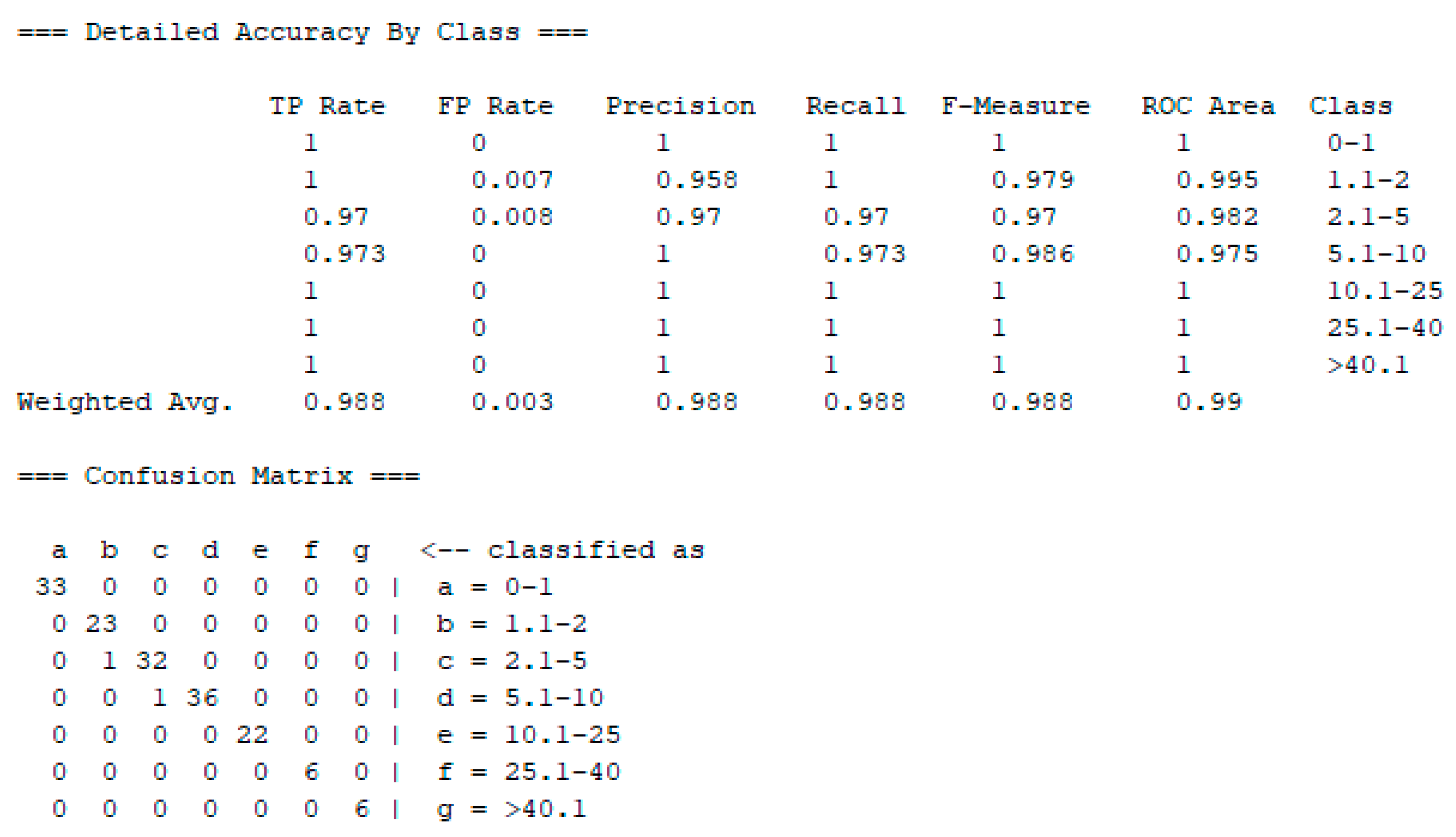
3.2.3. Prediction Accuracy

The BN model prediction accuracy is evaluated using statistical measures: Magnitude of Relative Error (MRE), Mean Magnitude of Relative Error (MMRE), Prediction at Level m (Pred. (m)), Accuracy, Mean Absolute Error (MAE), Root Mean Squared Error (RMSE), Relative Absolute Error (RAE) and Root Relative Squared Error (RRSE). Detailed descriptions of the measures, as well as the reasons for their use, are given in [7,21,36].

In this article, a Confusion Matrix is also used. The Confusion Matrix, just like the measures based on the prediction results in the confusion matrix, is well established as a measure of classification performance for imbalanced datasets [37,38]. The Confusion Matrix contains the prediction results and the actual values (classes) of these data. It is an nxn matrix, where n is the number of classes.

The model validation is performed using empirical data. WEKA provides a k-fold cross-validation and summary statistics (prediction accuracy, MAE, RMSE), which are used to verify the accuracy of the generated model. The WEKA error statistics are normalized. The predicted distribution for each class is matched against the expected distribution for that class. All the mentioned WEKA errors are computed by summing all classes of an instance, not just a true class [39].

In this case, a 10-fold cross-validation is used. The dataset is randomly divided into 10 equally sized subsets. Out of these 10 subsets, one is taken as the validation dataset, and the other nine sets are used as training data. Each of the nine training datasets is compared with a validation dataset to calculate the percentage of the model accuracy. The cross-validation process is repeated ten times, each of the ten subsets being used exactly once as a validation set. The results from all the 10 trials are averaged.

The measurement results are presented in

Table 5. Results.

	BN Model
	Old Model	New Model
Number of Tasks	160	160
Accuracy (Correctly classified instances)	99.375%	98.75%
MAE	0.026	0.037
RMSE	0.065	0.0792
RAE	9.71%	15.77%
RRSE	17.81%	23.13%
Pred. (25) %	40.625%	27.5%
MMRE	6.21	1.27

. Compared to the old BN model, the new one has a slightly worse, but still satisfactory, prediction accuracy. Only two tasks were misclassified, and the prediction accuracy is 98.75%, which is still an extremely accurate estimate.

The MAE values indicate that the expected effort will be within 3.7% of the true effort for the last set of data. Small differences between the MAE and the RMSE values indicate that the error variance is relatively small. The MMRE values suggest that the prediction error is relatively constant, with no occasional large deviations.

The diagonal of the confusion matrix shows correctly classified instances (Figure 3). The two misclassified tasks were placed in adjacent classes. There are no errors classified in remote classes.

The high accuracy of the model is confirmed via a comparison with the results listed in the literature [40].

Measure Pred (m) shows the worst results (Table 5). To determine the reason for this, Pred (25) was calculated to one instance from the task set. The instance lasted 0.5 h and was accurately classified into class ‘0–2’ in the old model (5 output intervals), i.e., into class ‘0–1’ in the new model (7 output intervals, Figure 4).

Pred. (m) measures the percentage of estimates for which the magnitude of the relative error MRE is less than or equal to m (usually m = 25) [41]. This BN model estimates effort as a set of probability distributions for all possible classes, so a conversion method is used to obtain the estimated effort as a discrete value [42,43,44]. The probabilities of the classes should be normalized so that their sum is equal to one. The estimated effort is then calculated as follows:

$$\mathrm{Effort}={{\displaystyle \sum }}_{\mathrm{i}=1}^{\mathrm{n}}{\mathsf{\rho }}_{\mathrm{classi}}{\mathsf{\mu }}_{\mathrm{classi}}$$

(2)

where µ_classi is the mean of class i, and ρ_classi is its respective class probability.

Each class probability of the selected instance is shown in

Table 6. The probability of each class of the selected instance.

The Old Model (5 Output Levels)		The New Model (7 Output Levels)
Class	Probability	Class	Probability
0–2	0.96	0–1	0.91
2.1–10	0.01	1.1–2	0.015
10.1–25	0.01	2.1–5	0.015
25.1–40	0.01	5.1–10	0.015
>40.1	0.01	10.1–25	0.015
		25.1–40	0.015
		>40.1	0.015

and the MRE is calculated according to the following equation:

$$\mathrm{MRE}=\frac{\left|{\mathrm{y}}_{\mathrm{i}}-\mathrm{f}\left({\mathrm{x}}_{\mathrm{i}}\right)\right|}{{\mathrm{y}}_{\mathrm{i}}}=\frac{\left|{\mathrm{y}}_{\mathrm{i}}-{{\displaystyle \sum }}_{\mathrm{i}=1}^{\mathrm{n}}{\mathsf{\rho }}_{\mathrm{classi}}{\mathsf{\mu }}_{\mathrm{classi}}\right|}{{\mathrm{y}}_{\mathrm{i}}}$$

(3)

where y_i is the actual value and f(x_i) is the estimated value.

The magnitude of the relative error for a correctly classified instance is 324.4% in the old model and 359.4% in the new one. It turns out that Pred (MRE < 25) is not a measure suitable for evaluating the performance of models with output classes. It is suitable for a relative comparison between two models with the same data set [45] or for the relative comparison of two data sets for the same model. Comparing the results of Pred. (25), the old model is more precise.

Consequently, it can be concluded that the BN model is suitable for estimating efforts on agile projects, and by increasing empirical data, it is easy to increase the number of output intervals, without affecting the accuracy of the estimate.

4. Application of BN Model in Another Company

The BN model is also tested on the empirical data of two companies, set A and set B. Set A is the data used in [23] and obtained from a micro software company that developed and improves an ERP system. For the development and improvement of that ERP system, the company uses Scrum agile methodology and many agile practices [46].

Set B is from another software company. It is a small software company engaged in software development for air traffic. The integrated software system supports the airport’s key business process, i.e., passengers and aircraft handling. The software is constantly updated and upgraded. The software is developed according to the principles of agile development and the set of used agile practices is selected according to the situation of the actual project. The following agile practices were used in the examples: daily meetings, simple design, testing, shared code ownership, ongoing integration, common room, sustainable pace, off-site customer, request prioritization, and request management [46].

During the work, the developers recorded the time spent on the development of each task. The project manager subsequently classified this information according to the rules set out by the authors. Thus, a 34-instance set was obtained and named set B.

Set B was used to test the new BN model. Although there were a small number of instances, the results were good. The prediction accuracy for the set B was 97.06%. Only one task was wrongly classified into an adjacent class.

Set B was added to set A (160 tasks) and the accuracy of the model was checked. In set A (7 output levels), two tasks were wrongly classified. By adding set B to set A, the number of misclassifications remained the same: the same two out of (now) 194 tasks were wrongly classified (Figure 5 and Figure 6).

5. Conclusions and Future Work

This paper develops a BN model for effort prediction in agile software development projects.

The proposed model is relatively small and simple, and all the input data are easily elicited. This way, the impact on agility is minimal. The model predicts task effort, and it is independent of the agile methods used.

The model is validated on real agile projects. It turns out that the structure and parameters of the model are well set, and the accuracy of the classification depends only on the number of instances available for learning. The conclusion is confirmed by the example of set A, where, by increasing the number of output classes from five to seven, the accuracy of the classification decreases by only 0.625%, i.e., from 99.375% to 98.75%. All misclassified instances are classified into adjacent classes.

Models using the BN for effort prediction have an accuracy range of 52% to 97% [40], so the authors will be pleased with a prediction accuracy of 80% or more (>98% is significantly over all expectations).

The model was also validated on the agile projects of another software company, resulting in set B. The applicability and success of the BN model were proven by combining the data from sets A and B. Tasks with varying contexts, including the following, were combined and had the same result:

• from different companies;
• of different types of software;
• from different areas of work,
• of different technologies;
• from different developers; and
• from different assessors/managers.

That way, the proposed BN model is validated.

It should be noted that models/methods for effort assessment are most often realized by using publicly available project databases. These databases have a defined structure, and researchers use mathematical methods to help them select the best solution. A different approach is applied in this research: variables for evaluation are defined from the known processes and data, a model is made, and then the success of the model is proven using mathematical measures.

Future work aims to investigate the impact of the productivity of both teams and individuals on effort estimation in agile software development.

References

1. Hamid, M.; Zeshan, F.; Ahmad, A.; Aimeur, E. Factors Contributing in Failures of Software Projects. IJCSNS Int. J. Comput. Sci. Netw. Secur. 2019, 19, 62–77. [Google Scholar]
2. Teslyuk, V.; Batyuk, A.; Voityshyn, V. Method of Software Development Project Duration Estimation for Scrum Teams with Differentiated Specializations. Systems 2022, 10, 123. [Google Scholar] [CrossRef]
3. Borade, J.G.; Khalkar, V.R. Software Project Effort and Cost Estimation Techniques. Int. J. Adv. Res. Comput. Sci. Softw. Eng. 2013, 3, 730–739. [Google Scholar]
4. Perkusich, M.; e Silva, L.C.; Costa, A.; Ramos, F.; Saraiva, R.; Freire, A.; Dilorenzo, E.; Dantas, E.; Santos, D.; Gorgônio, K.; et al. Intelligent Software Engineering in the Context of Agile Software Development: A Systematic Literature Review. Inf. Softw. Technol. 2020, 119, 106241. [Google Scholar] [CrossRef]
5. Saeed, A.; Butt, W.H.; Kazmi, F.; Arif, M. Survey of Software Development Effort Estimation Techniques. In Proceedings of the 2018 7th International Conference on Software and Computer Applications (ICSCA 2018), Kuantan, Malaysia, 8–10 February 2018; pp. 82–86. [Google Scholar]
6. Bashaera, A.; Kawtherb, S. Data-driven effort estimation techniques of agile user stories: A systematic literature review. Artif. Intell. Rev. 2022, 55, 5485–5516. [Google Scholar]
7. Rodríguez Sánchez, E.; Vázquez Santacruz, E.F.; Cervantes Maceda, H. Effort and Cost Estimation Using Decision Tree Techniques and Story Points in Agile Software Development. Mathematics 2023, 11, 1477. [Google Scholar] [CrossRef]
8. BaniMustafa, A. Predicting Software Effort Estimation Using Machine Learning Techniques. In Proceedings of the 2018 8th International Conference on Computer Science and Information Technology (CSIT), Amman, Jordan, 11–12 July 2018; pp. 249–256. [Google Scholar]
9. Cabral, J.T.H.; Oliveira, A.L.I. Ensemble Effort Estimation using dynamic selection. J. Syst. Softw. 2021, 175, 110904. [Google Scholar] [CrossRef]
10. Fenton, N.; Hearty, P.; Neil, M.; Radliński, Ł. Software Project and Quality Modelling Using Bayesian Networks. In Artificial Intelligence Applications for Improved Software Engineering Development: New Prospects, Information Science Reference; Meziane, F., Vadera, S., Eds.; IGI Publishing: Hershey, PA, USA, 2008; pp. 1–25. [Google Scholar]
11. Fenton, N.; Neil, M. A Critique of Software Defect Prediction Models. IEEE Trans. Softw. Eng. 1999, 25, 675–689. [Google Scholar] [CrossRef]
12. Celar, S.; Vickovic, L.; Mudnic, E. Evolutionary Measurement-Estimation Method for Micro, Small and Medium-Sized Enterprises Based on Estimation Objects. Adv. Prod. Eng. Manag. 2012, 7, 81–92. [Google Scholar] [CrossRef]
13. Jorgensen, M. What We Do and Don’t Know about Software Development Effort Estimation. IEEE Softw. 2014, 31, 37–40. [Google Scholar] [CrossRef]
14. Jorgensen, M. Selection of Strategies in Judgment-based Effort Estimation. J. Syst. Softw. 2010, 83, 1039–1050. [Google Scholar] [CrossRef]
15. Cohn, M. Agile Estimating and Planning, 1st ed.; Pearson: New York, NY, USA, 2005; ISBN 9780131479418. [Google Scholar]
16. Stephen, H.K. Metrics and Models in Software Quality Engineering, 2nd ed.; Addison-Wesley Longman Publishing Co., Inc.: Boston, MA, USA, 2002; ISBN 0201729156. [Google Scholar]
17. Jones, C. Applied Software Measurement—Global Analysis Of Productivity and Quality, 3rd ed.; McGraw-Hill Companies: New York, NY, USA, 2008; ISBN 0-07-150244-0. [Google Scholar]
18. McConnell, S. Software Estimation: Demystifying the Black Art; Microsoft Press: Redmond, WA, USA, 2006; ISBN 0735605351. [Google Scholar]
19. Jorgensen, M.; Shepperd, M. A Systematic Review of Software Development Cost Estimation Studies. IEEE Trans. Softw. Eng. 2007, 33, 33–53. [Google Scholar] [CrossRef]
20. Zarour, A.; Zein, S. Software Development Estimation Techniques in Industrial Contexts: An Exploratory Multiple Case-Study. Int. J. Technol. Educ. Sci. 2019, 3, 72–84. [Google Scholar]
21. Dragicevic, S.; Celar, S.; Turic, M. Bayesian Network Model for Task Effort Estimation in Agile Software Development. J. Syst. Softw. 2017, 127, 109–119. [Google Scholar] [CrossRef]
22. Ardiansyah, A.; Ferdiana, R.; Permanasari, A.E. MUCPSO: A Modified Chaotic Particle Swarm Optimization with Uniform Initialization for Optimizing Software Effort Estimation. Appl. Sci. 2022, 12, 1081. [Google Scholar] [CrossRef]
23. Rankovic, N.; Rankovic, D.; Ivanovic, M.; Lazic, L. A Novel UCP Model Based on Artificial Neural Networks and Orthogonal Arrays. Appl. Sci. 2021, 11, 8799. [Google Scholar] [CrossRef]
24. Perkusich, M.; Gorgonio, K.C.; Almeida, H.; Perkusich, A. Assisting the Continuous Improvement of Scrum Projects using Metrics and Bayesian Networks. J. Softw. Evol. Process 2017, 29, e1835. [Google Scholar] [CrossRef]
25. Radu, L. Effort Prediction in Agile Software Development with Bayesian Networks. In Proceedings of the 14th International Conference on Software Technologies (ICSOFT 2019), Prague, Czech Republic, 26–28 July 2019; pp. 238–245. [Google Scholar]
26. Malgonde, O.; Chari, K. An ensemble-based model for predicting agile software development effort. Empir. Softw. Eng. 2019, 24, 1017–1055. [Google Scholar] [CrossRef]
27. Durán, M.; Juárez-Ramírez, R.; Jiménez, S.; Tona, C. User Story Estimation Based on the Complexity Decomposition Using Bayesian Networks. Program Comput. Softw. 2020, 46, 569–583. [Google Scholar] [CrossRef]
28. Ratke, C.; Hoffmann, H.H.; Gaspar, T.; Floriani, P.E. Effort Estimation using Bayesian Networks for Agile Development. In Proceedings of the ICCAIS’ 2019 2nd International Conference on Computer Applications & Information Security, Riyadh, Saudi Arabia, 1–3 May 2019; pp. 1–4. [Google Scholar]
29. López-Martínez, J.; Ramírez-Noriega, A.; Juárez-Ramírez, R.; Licea, G.; Jiménez, S. User stories complexity estimation using Bayesian networks for inexperienced developers. Clust. Comput. 2018, 21, 715–728. [Google Scholar] [CrossRef]
30. Hearty, P.; Fenton, N.; Marquez, D.; Neil, M. Predicting Project Velocity in XP Using a Learning Dynamic Bayesian Network Model. IEEE Trans. Softw. Eng. 2009, 35, 124–137. [Google Scholar] [CrossRef]
31. Torkar, R.; Awan, N.M.; Alvi, A.K.; Afzal, W. Predicting Software Test Effort in Iterative Development Using a Dynamic Bayesian Network. In Proceedings of the 21st IEEE International Symposium on Software Reliability Engineering, San Jose, CA, USA, 1–4 November 2010. [Google Scholar]
32. Charniak, E. Bayesian Networks without Tears: Making Bayesian Networks more Accessible to the Probabilistically Unsophisticated. AI Mag. 1991, 12, 50–63. [Google Scholar]
33. Basili, V.R.; Caldiera, G.; Rombach, H.D. The Goal Question Metric Approach. In The Encyclopedia of Software Engineering; John Wiley & Sons: Hoboken, NJ, USA, 1994; Volume 1, pp. 469–476. [Google Scholar]
34. Differding, C.; Joisl, B.; Lott, C.M. Technology Package for the Goal Question Metric Paradigm; Technical Report 281/96; University of Kaiserslautern: Kaiserslautern, Germany, 1996. [Google Scholar]
35. Celar, S.; Turic, M.; Vickovic, L. Method for Personal Capability Assessment in Agile Teams Using Personal Points; 22nd Telecommunications Forum; IEEE: Beograd, Serbia, 2014; pp. 1134–1137. [Google Scholar]
36. Huynh Thai, H.; Silhavy, P.; Fajkus, M.; Prokopova, Z.; Silhavy, R. Propose-Specific Information Related to Prediction Level at x and Mean Magnitude of Relative Error: A Case Study of Software Effort Estimation. Mathematics 2022, 10, 4649. [Google Scholar] [CrossRef]
37. Picek, S.; Heuser, A.; Jovic, A.; Bhasin, S.; Regazzoni, F. The Curse of Class Imbalance and Conflicting Metrics with Machine Learning for Side-channel Evaluations. IACR Trans. Cryptogr. Hardw. Embed. Syst. 2019, 2019, 209–237. [Google Scholar] [CrossRef]
38. Orozco-Arias, S.; Piña, J.S.; Tabares-Soto, R.; Castillo-Ossa, L.F.; Guyot, R.; Isaza, G. Measuring Performance Metrics of Machine Learning Algorithms for Detecting and Classifying Transposable Elements. Processes 2020, 8, 638. [Google Scholar] [CrossRef]
39. WEKA. How to Do Proper Testing in Weka and How to Get Desired Results? Available online: https://stackoverflow.com/questions/10053125/how-to-do-proper-testing-in-weka-and-how-to-get-desired-results (accessed on 2 May 2023).
40. Radlinski, L. A Survey of Bayesian Net Models for Software Development Effort Prediction. Int. J. Softw. Eng. Comput. 2010, 2, 95–109. [Google Scholar]
41. Conte, S.D.; Dunsmore, H.E.; Shen, V.Y. Software Engineering Metrics and Models. Benjamin-Cummings Publishing Co., Inc.: San Francisco, CA, USA, 1986. [Google Scholar]
42. Pendharkar, P.C.; Subramanian, G.H.; Rodger, J.A. A Probabilistic Model for Predicting Software Development Effort. IEEE Trans. Softw. Eng. 2005, 31, 615–624. [Google Scholar] [CrossRef]
43. Mendes, E. The Use of Bayesian Networks for Web Effort Estimation: Further Investigation. In Proceedings of the Eighth International Conference on Web Engineering, Proceedings of ICWE’08, Washington, DC, USA, 14–18 July 2008; pp. 203–216. [Google Scholar]
44. Tierno, I.A.P. Assessment of Data-Driven Bayesian Networks in Software Effort Prediction. 2013. Available online: https://lume.ufrgs.br/handle/10183/71952 (accessed on 3 August 2023).
45. Chulani, S.; Boehm, B.; Steece, B. Bayesian analysis of empirical software engineering cost models. IEEE Trans. Softw. Eng. 1999, 25, 573–583. [Google Scholar] [CrossRef]
46. Williams, L. Agile Software Development Methodologies and Practices. Adv. Comput. 2010, 80, 1–44. [Google Scholar]
Figure 1. The old BN model adapted with permission from [21].
Applsci 13 09465 g001
Figure 2. The new BN model.
Applsci 13 09465 g002
Figure 3. Confusion matrix and accuracy measures per classes a–g.
Applsci 13 09465 g003
Figure 4. Number of tasks per interval.
Applsci 13 09465 g004
Figure 5. Misclassified instances in set A (160 instances).
Applsci 13 09465 g005
Figure 6. Set A + B—misclassified instance details (194 instances).
Applsci 13 09465 g006