
Performance of Iterative Coded CDMA Receivers with APP Feedback: A Use of a Weighted Delay Filter

Abstract
:1. Introduction
- Extrinsic feedback is used in a coded CDMA system.
- The notion of a ‘feedback residue’ for systems with APP feedback is introduced, and it is empirically shown that this residue term is a key consideration when determining the PIC output statistics.
- Using the ‘residual feedback’ model, it is shown that when APP feedback is utilised, data from previous cycles is not simply “a scaled, noisy version” of the current data. For this reason, benefits may be realised by APP feedback use.
- LLRs with Extrinsic Feedback are derived.
- It is demonstrated that extrinsic data, in the case of iterative receivers with suboptimal components, may not always yield the best results.
- It is analytically shown that when extrinsic feedback is used in a coded CDMA system, no benefit will be realised by weighted delay filtering, as soft outputs from previous cycles are a merely scaled, noisy version of the most recent data.
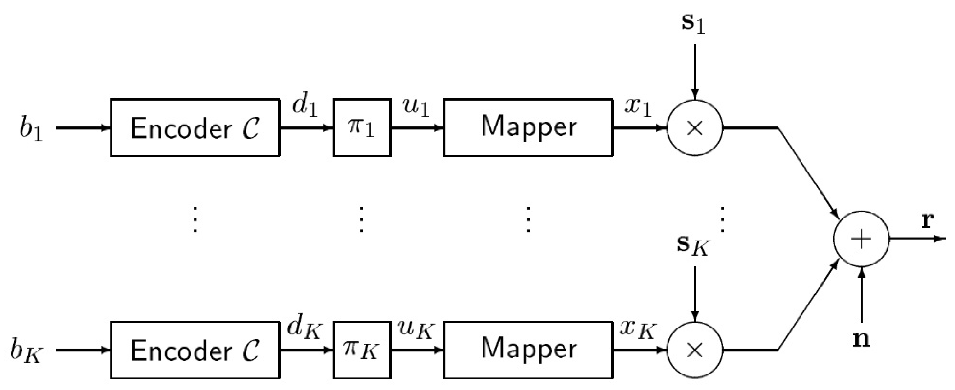
2. Coded CDMA
2.1. Optimal Detectors in Coded CDMA
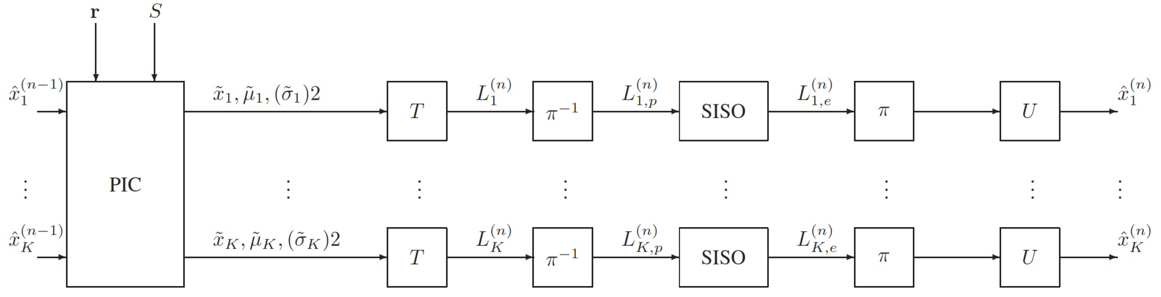
2.2. Suboptimal Detectors in Coded CDMA
3. Materials and Methods
3.1. Extrinsic Feedback, a Study
3.2. LLRs with Extrinsic Feedback
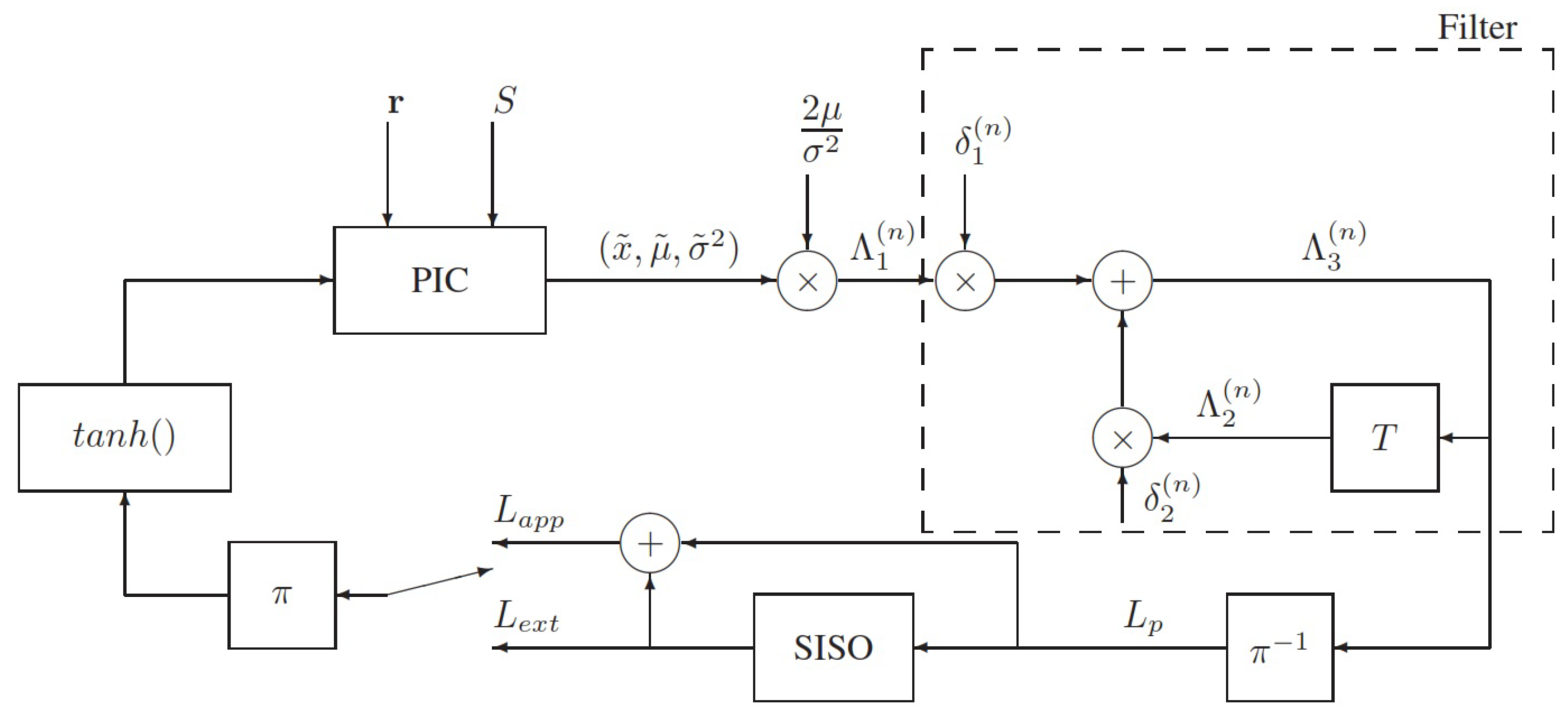
3.3. The APP Feedback Case
- What are the significant differences between the extrinsic feedback case and the APP feedback case?
- How does the analysis in Section 2.2 differ when APP feedback is used?
3.3.1. The PIC Output Mean with APP Feedback
3.3.2. The PIC Output Variance with APP Feedback
3.3.3. LLRs with APP Feedback
4. Results and Discussion
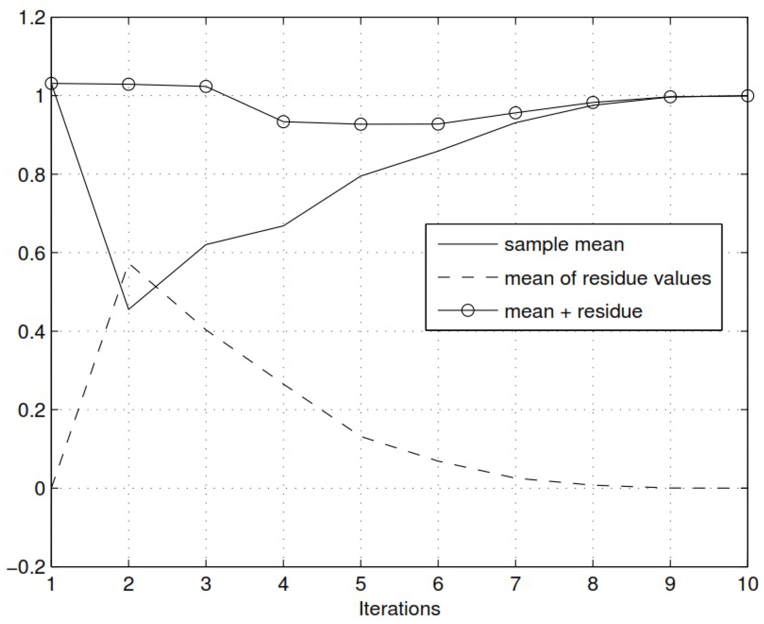
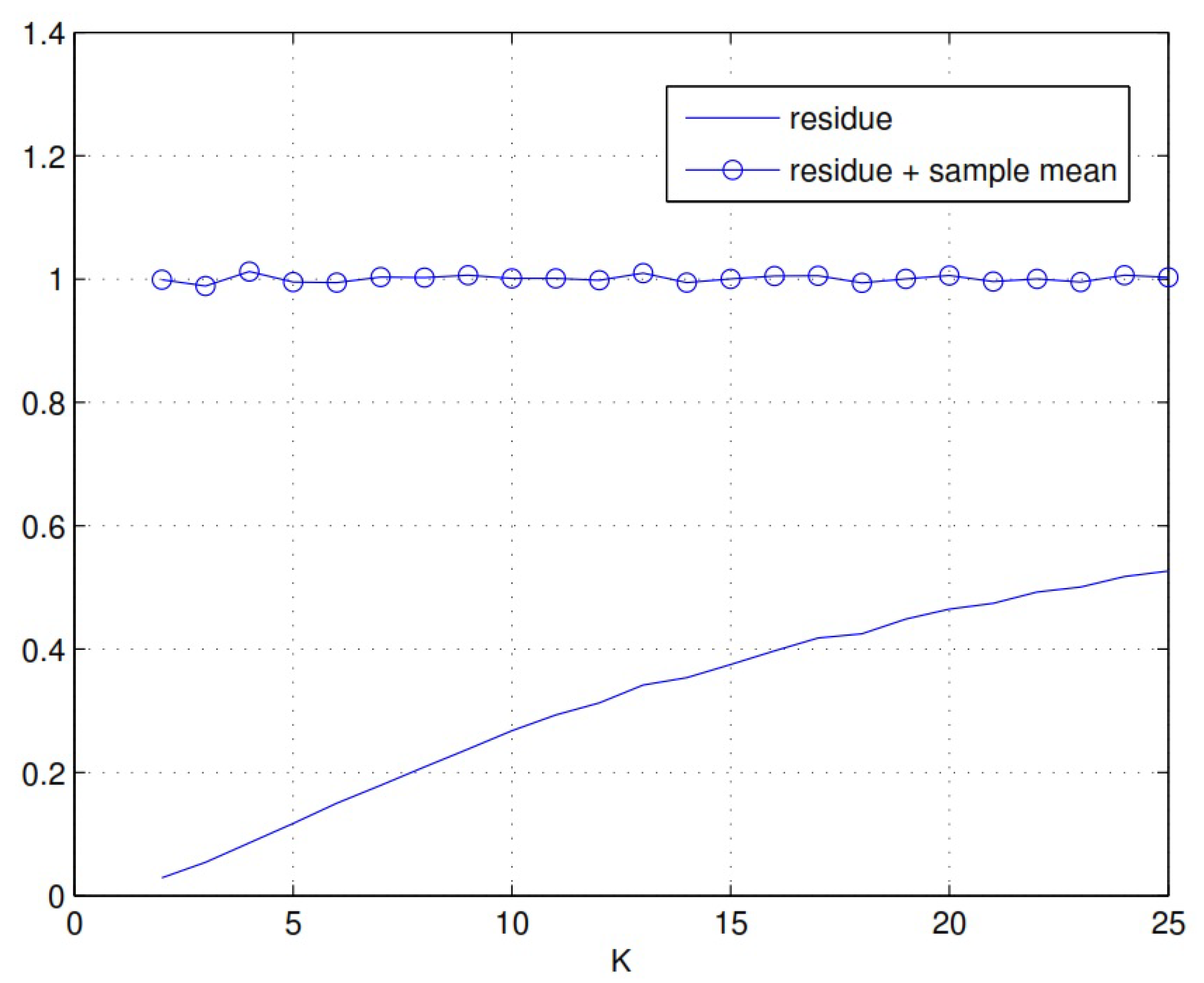
4.1. Behaviour of PIC Mean for APP Feedback
- This output mean drops below unity.
- This output mean value is the sum of the APP mean and the residue.
4.2. Behaviour of the Residue
5. Conclusions
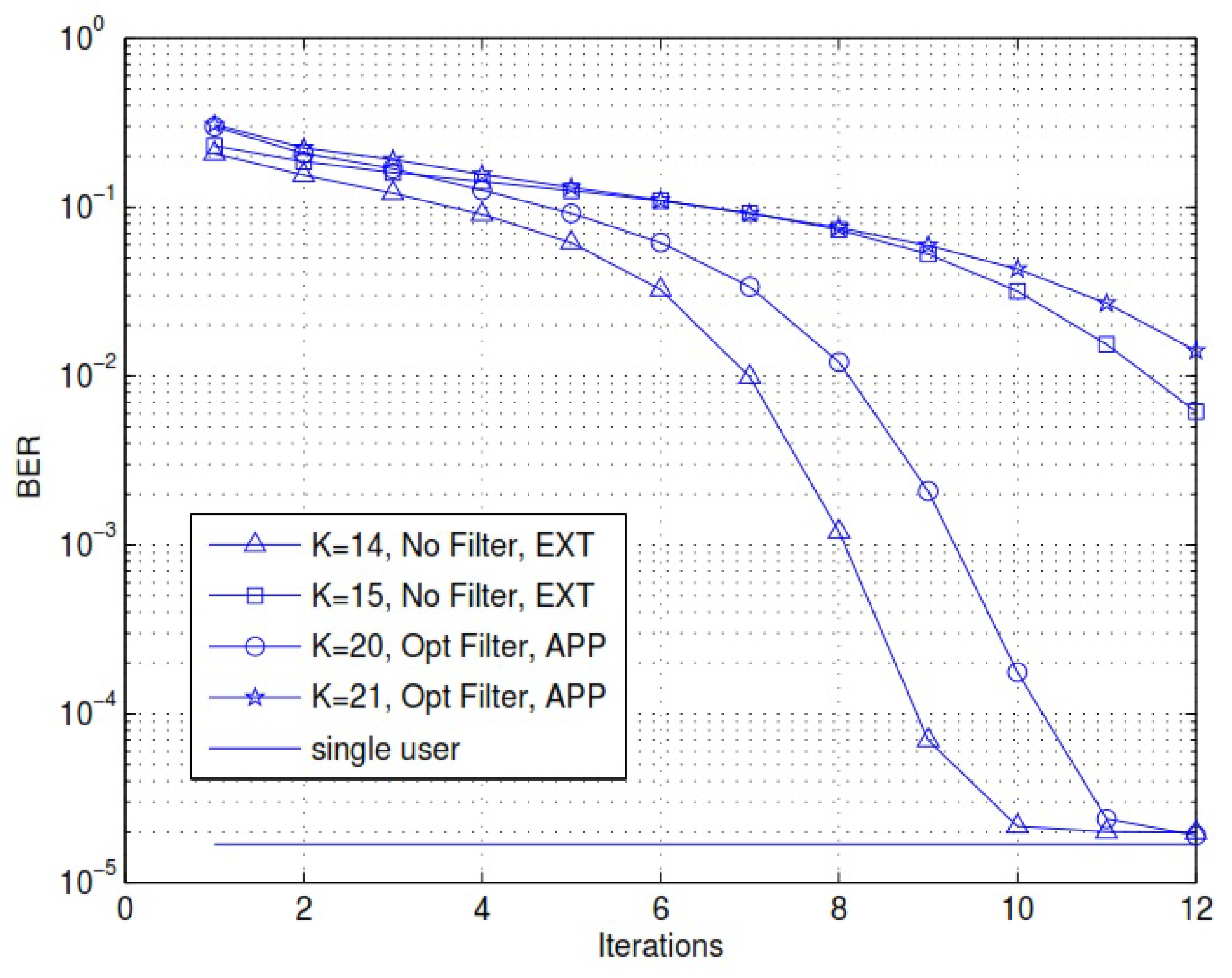
- The iterative receivers with suboptimal components may not always yield the best results.
- For a coded CDMA system with extrinsic feedback, no benefit will be realised by weighted delay filtering.
- Determining the PIC output statistics analytically in the case of APP feedback remains an open problem.
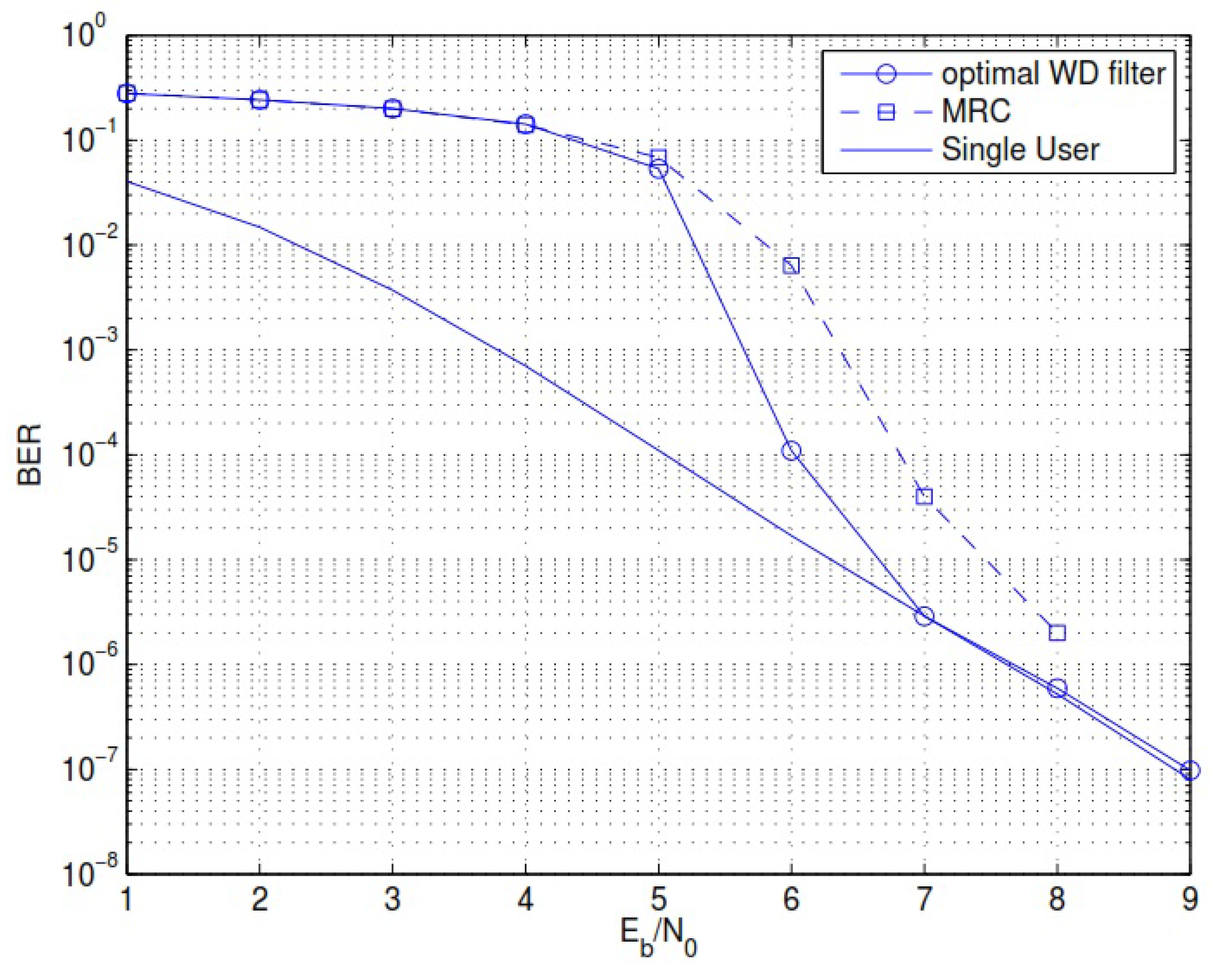
- The conclusion can be made that for a given values of SNR = 6 dB, and a processing gain of 10 dB, the system load increases to approximately 42% using the weighted delay filtering.
- Further noted that WDF outperforms MRC giving a value of 0.8 dB.
Author Contributions
Funding
Institutional Review Board Statement
Informed Consent Statement
Data Availability Statement
Conflicts of Interest
References
- Berrou, C.; Glavieux, A.; Thitimajshima, P. Near shannon limit error-correcting coding and decoding: Turbo codes. IEEE Int. Conf. Commun. 1993, 2, 1064–1070. [Google Scholar]
- Benedetto, S.; Divsalar, D.; Montorsi, G.; Pollara, F. Serial concatenation of interleaved codes: Performance analysis, design, and iterative decoding. IEEE Trans. Inf. Theory 1998, 44, 909–926. [Google Scholar] [CrossRef] [Green Version]
- Gallager, R. Low-Density Parity Check Codes; MIT Press: Cambridge, MA, USA, 1963. [Google Scholar]
- Divsalar, D.; Jin, H.; McEliece, R. Coding theorems for turbo-like codes. In Proceedings of the 36th Allerton Conference on Communication Control and Computing, Urbana, IL, USA, 23–25 September 1998; pp. 201–210. [Google Scholar]
- Moher, M. An iterative multiuser decoder for near-capacity communications. IEEE Trans. Commun. 1998, 46, 870–880. [Google Scholar] [CrossRef]
- Alexander, P.; Grant, A.; Reed, M. Iterative detection of codedivision multiple-access with error control coding. Eur. Trans. Telecommun. 1998, 9, 419–426. [Google Scholar] [CrossRef]
- Douillard, C.; Jezequel, M.; Berrou, C.; Picart, A.; Didier, P.; Glavieux, A. Iterative correction of intersymbol interference: Turboequalization. Eur. Trans. Telecommun. 1995, 6, 507–511. [Google Scholar] [CrossRef] [Green Version]
- Alexander, P.; Grant, A. Iterative channel and information sequence estimation in CDMA. In Proceedings of the IEEE 6th International Symposium on Spread Spectrum Techniques and Applications, Parsippany, NJ, USA, 6–8 September 2000. [Google Scholar]
- Gamal, H.E.; Hammons, A.R., Jr. A new approach to layered space-time coding and signal processing. IEEE Trans. Inf. Theory 2001, 47, 2321–2334. [Google Scholar] [CrossRef]
- Verdu, S. Multiuser Detection; Cambridge University Press: Cambridge, UK, 1998. [Google Scholar]
- Mu, H.; Tang, Y.; Li, L.; Ma, Z.; Fan, P.; Xu, W. Polar coded iterative multiuser detection for sparse code multiple access system. China Commun. 2018, 15, 51–61. [Google Scholar] [CrossRef]
- Park, H.J.; Lee, J.W. LDPC Coded Multi-User Massive MIMO Systems with Low-Complexity Detection. IEEE Access 2022, 10, 25296–25308. [Google Scholar] [CrossRef]
- Li, S.; Feng, Y.; Sun, Y.; Xia, Z. A low-complexity detector for uplink SCMA by exploiting dynamical superior user removal algorithm. Electronics 2022, 11, 1020. [Google Scholar] [CrossRef]
- Zheng, Y.; Xin, J.; Wang, H.; Zhang, S.; Qiao, Y. A low-complexity codebook design scheme for SCMA systems over an AWGN channel. IEEE Trans. Veh. Technol. 2022, 71, 8675–8688. [Google Scholar] [CrossRef]
- Yue, M.; Liu, L.; Yuan, X. RIS-Aided Multiuser MIMO-OFDM with Linear Precoding and Iterative Detection: Analysis and Optimization. IEEE Trans. Wirel. Commun. 2023. [Google Scholar] [CrossRef]
- Marey, M.; Mostafa, H. A Powerful Joint Modulation and STBC Identification Algorithm for Multiuser Uplink SC-FDMA Transmissions. Appl. Sci. 2023, 13, 1853. [Google Scholar] [CrossRef]
- Giallorenzi, R.T.; Wilson, G.; Multiuser, S. ML sequence estimator for convolutionally coded asynchronous DS-CDMA systems. IEEE Trans. Commun. 1996, 44, 997–1008. [Google Scholar] [CrossRef]
- Chi, Y.; Liu, L.; Song, G.; Li, Y.; Guan, Y.L.; Yuen, C. Constrained Capacity Optimal Generalized Multi-User MIMO: A Theoretical and Practical Framework. IEEE Trans. Commun. 2022, 70, 8086–8104. [Google Scholar] [CrossRef]
- Qin, Y.; Qin, Z.; Zhang, Z.; Li, Y.; Lu, Q. Evolutionary Programming: A Population-Based Optimization Algorithm for Coded Multiuser Systems. J. Commun. 2021, 16, 369–378. [Google Scholar] [CrossRef]
- Colavolpe, G.; Foggi, T.; Piemontese, A.; Ugolini, A.; Liu, L.; Han, J. Multiuser Detection for Time-Frequency-Packed Systems. IEEE Trans. Commun. 2022, 70, 6693–6703. [Google Scholar] [CrossRef]
- Liu, Q.; Feng, Z.; Xu, J.; Zhang, Z.; Liu, W.; Ding, H. Optimization of Non-Binary LDPC Coded Massive MIMO Systems with Partial Mapping and REP Detection. IEEE Access 2022, 10, 17933–17945. [Google Scholar] [CrossRef]
- Bahl, L.; Cocke, J.; Jelinek, F.; Raviv, J. Optimal decoding of linear codes for minimizing symbol error rate. IEEE Trans. Inf. Theory 1974, 20, 284–287. [Google Scholar] [CrossRef] [Green Version]
- Lin, T.; Rasmussen, L.K. Iterative Multiuser Decoding with Maximal Ratio Combining. In Proceedings of the Australian Communications Theory Workshop, Newcastle, Australia, 4–6 February 2004; pp. 42–46. [Google Scholar]
- Lin, T.; Rasmussen, L.K. Truncated Maximal Ratio Combining for Iterative Multiuser Decoding. In Proceedings of the Australian Communications Theory Workshop, Brisbane, Australia, 2–4 February 2004; pp. 35–41. [Google Scholar]
- Proakis, J.G. Digital Communications, 4th ed.; McGraw-Hill: New York, NY, USA, 2001. [Google Scholar]
- Hagenauer, J. Forward error correcting for CDMA systems. In Proceedings of the ISSSTA’95 International Symposium on Spread Spectrum Techniques and Applications, Mainz, Germany, 25 September 1996; Volume 2, pp. 566–569. [Google Scholar]
- Joo, W.Y.; Yoon, S.Y.; Lee, H.S. A weighted parallel interference cancellation detector for convolutionally coded CDMA systems. In Proceedings of the VTC2000-Spring—IEEE 51st Vehicular Technology Conference Proceedings (Cat. No. 00CH37026), Tokyo, Japan, 15–18 May 2000; Volume 2, pp. 1100–1104. [Google Scholar]
- Juntti, M.; Kaurahalme, O.P. Performance of parallel interference cancellation for CDMA with channel coding. In Proceedings of the IEEE 49th Vehicular Technology Conference (Cat. No. 99CH36363), Houston, TX, USA, 16–20 May 1999; Volume 2, pp. 1440–1444. [Google Scholar]
- Xu, G.; Gan, L. New parallel interference cancellation/decoding for convolutionally coded CDMA systems over fading channel. In Proceedings of the International Conference on Communication Technology, Guilin, China, 27–30 November 2006; pp. 1–4. [Google Scholar]


| Accronyms | Description | Accronyms | Description |
|---|---|---|---|
| APP | A-Posterior Probability | CDMA | Code Division Multiple Access |
| C-CDMA | Coded-CDMA | BER | Bit Error Rate |
| SNR | Signal-to-noise Ratio | MUD | Multi User Detection |
| PIC | Parallel Interference Cancellation | LLR | Log-likelihood Ratio |
| MAI | Multiple Access Interference | SISO | Single Input Single Output |
| Symbol | Description | Symbol | Description |
|---|---|---|---|
| LLR | Correlation Factor | ||
| Mean | Variance | ||
| Normal RV | Expected Value | ||
| Received Signal | X | Symbol | |
| Scaled value of LLR | System load | ||
| N | Gain | K | No. of users |
| L | Data Sequence Length | x | BPSK sybmol |
| Estimated of x | LLR at output of PIC | ||
| LLR from previous iteration | SNR of |
| Systems | Maximum Users | Systems | Maximum Users |
|---|---|---|---|
| PIC with no Combining | 9 | PDA with no Combining | 16 |
| PIC with Full MRC | 13 | PDA with Full MRC | 17 |
| PIC with TMRC | 15 | PDA with TMRC | 17 |
Disclaimer/Publisher’s Note: The statements, opinions and data contained in all publications are solely those of the individual author(s) and contributor(s) and not of MDPI and/or the editor(s). MDPI and/or the editor(s) disclaim responsibility for any injury to people or property resulting from any ideas, methods, instructions or products referred to in the content. |
© 2023 by the authors. Licensee MDPI, Basel, Switzerland. This article is an open access article distributed under the terms and conditions of the Creative Commons Attribution (CC BY) license (https://creativecommons.org/licenses/by/4.0/).
Share and Cite
Altalbe, A.; Tahir, M. Performance of Iterative Coded CDMA Receivers with APP Feedback: A Use of a Weighted Delay Filter. Appl. Sci. 2023, 13, 9175. https://doi.org/10.3390/app13169175
Altalbe A, Tahir M. Performance of Iterative Coded CDMA Receivers with APP Feedback: A Use of a Weighted Delay Filter. Applied Sciences. 2023; 13(16):9175. https://doi.org/10.3390/app13169175
Chicago/Turabian StyleAltalbe, Ali, and Muhammad Tahir. 2023. "Performance of Iterative Coded CDMA Receivers with APP Feedback: A Use of a Weighted Delay Filter" Applied Sciences 13, no. 16: 9175. https://doi.org/10.3390/app13169175