1. Introduction
Deep learning models have made significant advances in a variety of computer vision tasks, including image classification, object recognition, semantic segmentation, and ancillary tasks such as visual question answering and autonomous driving. Artificial intelligence (AI) is now widely used in our daily lives. To put this into perspective, the International Data Corporation (IDC) predicts that global investment in AI will rise to USD 154 billion by 2023. Meanwhile, according to Statista, global AI market revenues are expected to reach USD 1.8 trillion dollars in 2030 [
1]. This will influence the next generation of digital business models and ecosystems, alongside immersive experiences, digital twins, event thinking, and continuous adaptive security [
2].
On the other hand, deep neural networks (DNNs) are difficult to understand because they behave like black boxes. Most researchers emphasise the framework and many internal parameters of the model when building deep neural network models, but if the model is incorrect, they are unable to make a correct interpretation of the model’s output. Determining confidence in individual predictions is an important issue when using the model for decision making. For example, when applying machine learning to medical diagnosis or terrorism detection, predictions cannot be trusted because their impact can be catastrophic.
Despite the apparent effectiveness of AI algorithms in terms of outcomes and predictions, there remains an opacity that makes it difficult to gain insight into their core operating mechanisms. As a result, users in healthcare, banking, and security are unable to trust the decisions made by the models. We need to create transparent models that show consumers how algorithms think. The creation of transparent models would benefit from an understanding of errors, debugging, and the discovery of potential biases in the training data.
XAI advocates a move away from transparent artificial intelligence. The goal is to build more understandable models while maintaining high levels of performance, making the decisions of DNN models more transparent, understandable, and trustworthy to humans.
In this paper, we propose specific-input LIME, a novel XAI method for interpreting deep learning models based on tabular data, by combining the specific-input procedure with the LIME method. The specific-input LIME method replaces some of the steps in LIME with feature importance and PDP. First, we obtain the basic interpretation of the data by simulating user behaviour. Second, we use feature importance and PDP to understand “what” features deep learning models focus on and how they affect the model’s predictions. Analysis of the experimental results shows that our approach provides more detailed explanations than the LIME approach, and also compensates for the vulnerability of LIME to random sampling.
2. Literature Review of Explainability
Two inescapable position papers that attempt to formalise the concept of interpretability are [
3,
4]. The former aims to provide a taxonomy of interpretability research aspirations and techniques. Lipton’s study is not a survey per se. However, it provides a reliable assessment of what interpretability means through the lens of the literature [
3].
Doshi-Velez and Kim conducted a survey to establish taxonomies and best practices for interpretability as a “rigorous science” [
4]. The main contribution of this paper is the evaluation of interpretability taxonomies. Therefore, the authors focus on one aspect of scalability: measurement.
In a 2018 survey, Guidotti et al. [
5] explored strategies for interpreting black-box models in a wide range of domains, including data mining and machine learning. They provide a classification of explainable strategies based on the problems they address. Although the survey assesses completeness from a modelling perspective, it focuses only on the process of interpretability and ignores additional dimensions of interpretability, such as evaluation. Thus, a thorough technical overview of the techniques examined makes it difficult to quickly grasp the interpretive method space.
2.1. Interpretability Strategies
With the urgent need for interpretability in AI systems, a large number of interpretability methods and strategies have emerged in a short period of time, mainly targeting machine learning algorithms. The purpose of this section is to provide an overview of these interpretability methods. Indeed, much research has been devoted to improving the interpretability of machine learning methods.
Based on our literature review, we classify these methods according to three criteria: (i) the complexity of interpretability, (ii) the scope of interpretability, and (iii) model-based methods. The main features of each category are described in the following subsections, along with examples from current research.
2.2. The Complexity of Interpretability
The interpretability of a machine learning model is proportional to its complexity. The more complex a model is, the more difficult it is to understand and explain. Therefore, the most direct path to interpretable AI is to create an algorithm that is naturally and inherently interpretable.
Letham et al. proposed a decision-tree-based model called Bayesian rule lists (BRL), claiming that the preliminary interpretable model provides a simple and persuasive way to gain the trust of domain experts [
6].
Caruana et al. used a learning strategy based on generalised additive models for the pneumonia problem. They used case studies on real medical data to demonstrate the model’s comprehensibility [
7].
Xu et al. proposed an attention-based approach that learns to describe image information automatically [
8]. They demonstrated how the model could comprehend the results using visualisation.
Due to its high level of sparsity and small integer coefficients, Ustun and Rudin presented a sparse linear model for creating data-driven scoring systems called SLIM [
9]. The results of this study underline the explainability of the proposed system in providing users with an insightful understanding.
This suggests that the nature of the prediction effort affects the overall usefulness of interpretability. Inherently decipherable models are adequate as long as they maintain accuracy for the task and require a minimal amount of internal elements. It is also worth noting that there is a collection of intrinsic approaches to complex uninterpretable models in the literature. These methods attempt to increase the interpretability of a sophisticated black-box model that is not primarily interpretable, such as a DNN, by modifying the internal structure of the model.
2.3. The Scope of Interpretability
Interpretability refers to the ability to understand an automated model. There are two types of interpretability: understanding the complete behaviour of the model or understanding a specific prediction. In the literature reviewed, contributions are made in both directions. Consequently, interpretability is divided into two categories: (i) global interpretability and (ii) local interpretability.
When deep learning models are needed to inform population-level decisions, such as drug consumption trends or climate change, this family of approaches comes in handy. In such circumstances, a global effect estimate might be more valuable than a long list of possible reasons. The pneumonia risk prediction model and the rule set built from a sparse Bayesian generative model proposed in
Section 2.2 are examples of work that provides globally interpretable models.
Yang et al. proposed using recursive partitioning to generate a global interpretation tree for a wide range of ML models based on their local explanations [
10]. In their experiments, the authors showed that their approach can detect whether a particular machine learning model is working sensibly or being overly adapted to an illogical pattern.
While various methods have been used in the literature to promote global interpretability, global models can be challenging in practice, especially for models with more than a few parameters. Local interpretability can be more easily applied, similar to human efforts to understand the whole model by focusing on only part of it.
Explainability occurs locally when explaining the reasoning behind a particular prediction. This aspect of interpretability is used to generate a unique explanation of why the model makes a particular decision in a particular situation. Several studies have proposed local explanatory approaches. The following section summarises the explanatory approaches examined in the peer-reviewed studies.
LIME stands for local interpretable model-agnostic explanations, as presented by Ribeiro et al. [
11]. This model can approximate a black-box model near any prediction.
Baehrens et al. make another attempt to generate local explanations. The authors provide a method that uses local gradients to specify how a data point must move to change its predicted label, in order to explain the local decisions made by arbitrary nonlinear classification algorithms [
12]. In this vein, we find a number of studies of image classification models that use a similar strategy. Locating regions of an image that have a strong influence on the final classification is a typical technique for understanding the decisions of image classification algorithms.
Combining the strengths and benefits of both local and global interpretability is an exciting and promising research path. The following are the four possible combinations: (i) How does the model create predictions? (ii) On a modular level, global model interpretability identifies how different elements of the model influence predictions. (iii) For a group of predictions, local interpretability reveals why the model made specific conclusions for a set of cases. (iv) Finally, the model’s usual local interpretability for a single prediction is utilised to demonstrate why it drew a given conclusion for a particular case [
13].
Another point worth mentioning is that local explanations are the most common way of generating explanations in DNNs in the literature reviewed. Although these methods were developed to explain neural networks, authors often emphasise that they can be used to explain any type of model, making them agnostic models.
3. Materials and Methods
3.1. Local Interpretable Model-Agnostic Explanations
Artificial intelligence cannot evolve without trust, so models that do not provide a clear rationale for their decisions will not be trusted. To address the trust problem, the local interpretable model-agnostic explanations (LIME) approach has been proposed. LIME is a human-centred approach that tries to bridge the gap between AI and humans. LIME focuses on two key areas: model confidence and prediction confidence. LIME provides a unique explainable AI system that explains predictions at the local level. The next section defines LIME and its unique approach.
A deep learning model typically learns at least ten features to make a prediction. If all of these features are displayed in an interface, it is practically difficult for a user to visually verify the result. Compared to previous XAI approaches, LIME takes a unique approach.
LIME needs to know if a model is a local fidelity independent of the model. Local fidelity does a good job of checking that a model reflects features close to a prediction. However, local fidelity may not fit the model perfectly, and may only explain how the prediction was produced. LIME examines the immediate context of a forecast to explain it and assess its local fidelity. Consider the scenario where a prediction is accurate but for a reason other than our global model. To explain the model’s decision, LIME will look for it in the region of the predicted instance and may also find high-probability features in that scenario.
3.2. Mathematical Representation of LIME
This section explains our understanding of LIME in mathematical terms.
The original, global representation of a given instance
x is as follows:
A binary vector, on the other hand, is an explainable representation of an instance:
The explainable representation indicates whether a feature or set of features is present or absent at a given location.
Let us have a look at LIME’s model-agnostic property. A deep learning model is represented by the letter
g.
G denotes a set of models that includes
g as well as other models:
As a result, any other model will be explained similarly by LIME’s algorithm. Because the gg domain is a binary vector, we can write it as follows:
The complexity of
may make studying the neighbourhood of an instance difficult. This is something we must consider. As an example of the complexity of a model explanation, consider the following:
For humans to be able to explain a forecast, must be low enough.
The model can thus also be defined as follows:
The significance of a proximity measurement between an instance
z and the neighbourhood around
x may be seen. This proximity measurement will be defined as follows:
Except for one crucial variable, we now have all the variables we need to define LIME. How close is this prediction to our model’s global ground truth? Is it possible to explain why it is reliable? Our challenge will be answered by determining how unreliable a model g can be when estimating f in the locality .
A prediction could be a false positive, for all we know! It is also possible that the prognosis is a false negative! Worse yet, the prediction could be a true positive or negative for the wrong reasons.
We use the letter L to represent unfaithfulness. will determine how untrustworthy g is when approximating f in the area we described as .
Finally, we may define a LIME-generated explanation
as follows:
The above is a complete mathematical representation of the LIME method by Ribeiro et al. [
11]. Regardless of the model used, LIME will draw samples weighted by
to optimise the equation and offer the best interpretation and explanations
. LIME can analyse a wide range of models, fidelity functions, and complexity metrics.
3.3. The Disadvantages of LIME
Tabular data represent information in the form of tables, where each row represents an instance and each column represents a feature, and there are complex relationships between tabular data, whereas LIME assumes that all features are independent, which obviously reduces the accuracy of interpretation for tabular data. Although it improves the possibility that some sample point predictions may deviate from the data points of interest, LIME samples are taken from the centre of mass of the training data rather than from the instances of interest, leading to problems of consistency, confidence, and stability of interpretation.
It is easiest to describe how sampling and local model training work with
Figure 1 (represented by Molnar C. [
13]):
In
Figure 1, the black-box model predictions are based on x1 and x2, where x1 and x2 represent the two features or input variables used to make the predictions. The predicted classes (light) are 1 (dark) or 0 (bright). Subfigure A means that the data are sampled from a normal distribution and a point of interest (large dots) is sampled (small dots). In subfigure B, more weight is given to the points closer to the point of interest. In subfigure C, the grid marks show the classifications of the locally learned model from the weighted samples. In subfigure D, the decision boundary is marked by a white line (P(class = 1) = 0.5).
It is difficult to define a meaningful neighbourhood around a point. To define the neighbourhood, LIME currently uses an exponential smoothing kernel [
14]. A smoothing kernel is a function that returns a measure of the closeness of two data instances. The kernel width is a measure of the size of the neighbourhood: a minimal kernel width means that an instance must be in close proximity to affect the local model, while an extended kernel width means that instances at greater distances can also affect the model.
We found that it uses an exponential smoothing kernel with a width of 0.75 times the square root of the number of columns in the training data. The main problem is that we do not have a good method for the determination of the correct kernel or width. In some cases, the adjustment of the kernel width can have a positive effect on the explanation, as shown in
Figure 2 (represented by Molnar C. [
13]):
The predictions of the black-box model based on a single feature are shown by a thick line, while carpets represent the data distribution. Three local surrogate models are generated, each with a different kernel width.
In this example, there is only one feature. In a high-dimensional feature space, the situation becomes worse. It is also uncertain whether all features should be treated equally in the distance measurement. Distance measurements are arbitrary and distances in different dimensions may not be comparable.
The correct definition of neighbourhoods is a huge, unresolved problem when using LIME with tabular data, which is LIME’s most serious flaw and why experts recommend using it only with extreme caution. You need to experiment with different kernel settings for each application to see if the interpretation makes sense.
In the existing implementation of LIME, there is room for improvement in the sampling technique. Currently, data points are generated according to a Gaussian distribution without any consideration of feature correlation. This approach can lead to the creation of unlikely data instances that can be used to learn local explanatory models despite their improbability.
The complexity of the explanatory model must be determined in advance. This is a minor problem because the end user has to choose between truthfulness and sparsity. Another important issue is the instability of the interpretation. Furthermore, in our experience, results can vary when the sampling process is repeated. The uncertainty makes it difficult to accept interpretations and you should be sceptical. Data scientists can change the interpretation of LIME to hide bias. Accepting LIME-generated interpretations is more difficult because of the potential for manipulation.
3.4. Specific-Input LIME
3.4.1. The Architecture of Specific-Input LIME
Here, we present the structure of the specific-input LIME, with our approach focusing on feature importance and partial dependency plot (PDP) values as a complement to the shortcomings of the LIME approach.
The specific-input LIME method is primarily used to analyse data learned from black-box models, but unlike conventional methods, the specific-input LIME method allows for greater interpretability of the data points used in the LIME method.
The structure of the specific-input LIME is shown in
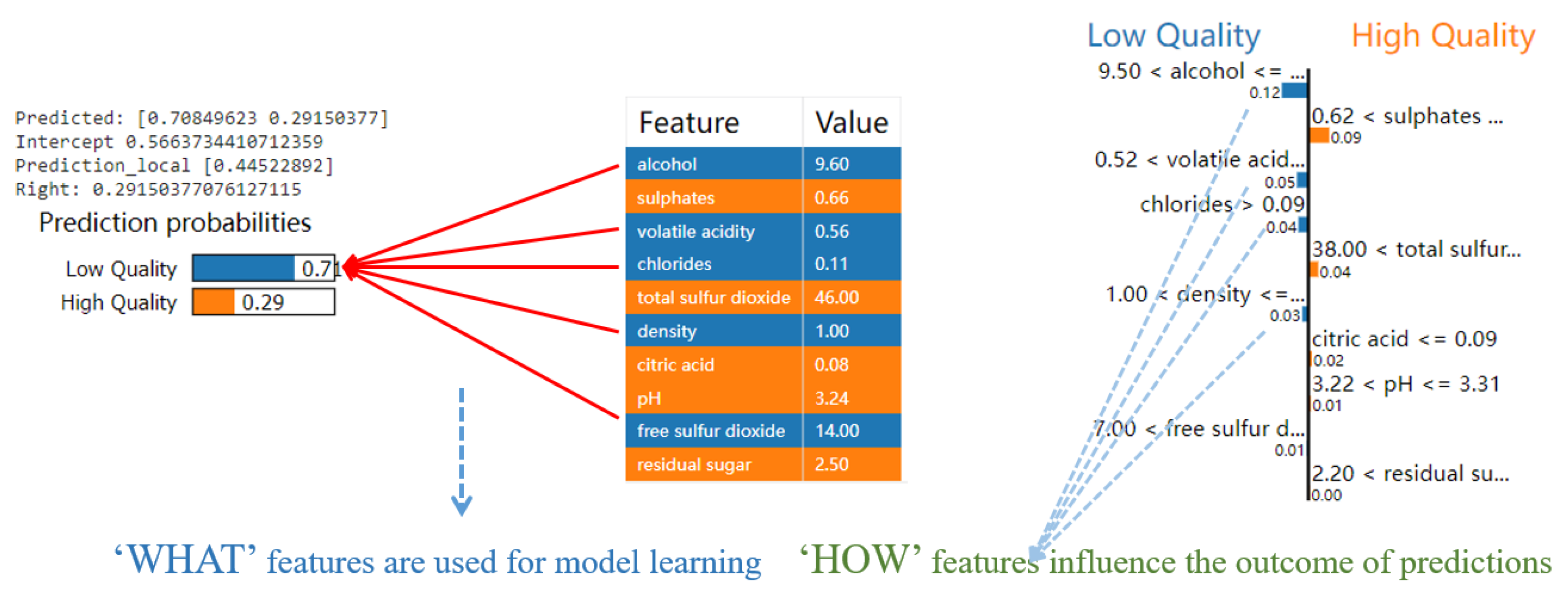
Figure 3:
The specific-input LIME has three main parts: feature importance, PDP and LIME. The feature importance part also uses the gain feature importance and split feature importance. The PDP part uses a binary PDP, which is used to partition the data learned by the black-box model into regions. The feature importance and the binary PDP are then integrated into the LIME method to obtain the final interpretation. Specifically, feature importance plots show ‘what’ features affect predictions the most. Partial dependence plots (PDP) show ‘how’ a feature affects predictions.
3.4.2. Feature Importance
Feature importance refers to the methods used to calculate a score for each of the input features in a model. The scores are a measure of the ‘importance’ of each feature. A higher score is an indication that a particular feature will have a greater impact on the model used to predict a particular variable. Feature importance ranks features according to their impact on the prediction of the model.
In the feature importance part, we use both gain feature importance and split feature importance. In our experiments, we use the trained LightGBM Classifier model as a black-box model for explanation. We obtain the “gain/split feature importance” of the LightGBM Classifier model by calling the “plot importance” function of the LightGBM model.
The principle of split feature importance is that if a feature is used multiple times in the model for segmentation, the feature is considered relatively important. The principle of gain feature importance is based on the loss of the objective function at the point of feature splitting; if a feature splitting point can significantly reduce the loss of the objective function, the feature is considered to be relatively important. In this step, we filter out the features that have more influence on the model and then proceed to the later steps.
We selected features that had a greater impact on the model predictions based on the ranking of the importance of these features. For example, in the Wine Quality Dataset, the features ‘alcohol’ and ‘sulphates’ had the highest gain and segmentation importance in our model, so we selected these two features for further in-depth analysis. The selection of these important features not only helped us to optimise the performance of our model, but also enabled us to gain a deeper understanding of the working mechanism of the model.
3.4.3. Partial Dependency Plot
After the feature importance step, we draw the partial dependency plots of the features that have a greater impact on the model. The partial dependency plot (PDP) describes the marginal impact of one or two features on the expected outcome of a machine learning model [
15]. A PDP can determine whether the relationship between the target and the features is a linear one, a monotone one or a complex one. For example, when applied to linear regression models, PDPs will always show a linear relationship.
The partial dependence function for regression is defined as
The characteristics for which partial dependence function should be drawn are , and the other features utilised in the machine learning model, , which are represented as random variables here, are .
In most cases, the set S contains only one or two features. The feature in S for which we wish to know the effect on prediction is that in S. The complete feature space x comprises the feature vectors and . The function reveals the association between the features in set SS we are interested in and the expected outcome by marginalising the machine learning model output over the distribution of the features in set C. By marginalising the other features, we obtain a function that depends solely on features in S, including interactions with other features.
The partial function
is calculated using the Monte Carlo approach, which involves calculating averages in the training data:
The partial function shows us the average marginal effect on prediction for a given value of characteristics S. is the actual feature values from the dataset for the characteristics we are not interested in, and n is the number of instances in the dataset in this formula. The PDP assumes that the features in C are unrelated to the features in S.
The partial dependence plot illustrates the probability for a specific class given different values for the feature in S for classification when the machine learning model produces probabilities. Drawing one line or plot per class is a simple technique to deal with several classes.
We obtain the turning points of the folds of the feature’s PDP graph by means of the feature’s partial dependency plot (PDP) and analyse and compute the turning points in detail (see Algorithm 1 for the procedure), and present them together with the results of the LIME analysis to obtain the results of the interpretations at both the global and local levels. In fact, this approach also improves the stability of LIME in two ways:
(1) Feature space partitioning: By dividing the feature space into different intervals and performing the specific-input function separately in each interval, we essentially reduce the complexity of the prediction task within each interval. This leads to a more reliable approximation of the model’s behaviour in each interval, as it is less affected by changes that may occur in other regions of the feature space.
(2) Capturing local changes: This method also helps to capture local changes in the model behaviour in different intervals. By running the specific-input function on each interval, we are able to capture the effect on the predicted probabilities of specific feature values varying in different regions of the feature space. This allows us to understand the behaviour of the model at a more granular level than when considering the entire feature space as a whole.
| Algorithm 1: Calculate Prediction Probability Percentage_Change |
- 1:
Initialise an empty list named data_frame.array - 2:
Create a deep copy of the dataset named fake_data_frame - 3:
for each index i of feature content in fake_data_frame do - 4:
if feature content is between interval_min and interval_max then - 5:
Set the feature content in fake_data_frame to interval_min + interval_max divided by 2 - 6:
Append index i to the data_frame.array - 7:
end if - 8:
end for - 9:
Calculate the probabilities of the original dataset at indices in array using the model - 10:
Calculate the probabilities of the fake_data_frame dataset at indices in array using the model - 11:
Calculate the change in feature values between original and fake_data_frame - 12:
Take the absolute value of feature change and compute the sum - 13:
Calculate the change in probabilities and divide by 2 - 14:
Calculate the total change (probability change divided by feature change) - 15:
Calculate the percentage_change (total change divided by the length of array)
|
Using a combination of PDP and LIME provides a more complete understanding of the model’s behaviour: the PDP identifies general trends in the data, and the LIME provides specific explanations for individual observations or localised regions of feature space. This approach is well suited to explaining complex models where there is no clear relationship between some features and the outcome variable.
4. Results and Discussion
In this section, we present simulated user tests to assess the usefulness of explanations in classification tasks. In particular, we address the following question: can the explanations help users decide whether or not to believe the predictions?
4.1. Data Description
The dataset used in this experiment is the Wine Quality Dataset used in [
16]. This dataset is publicly available and can be used for research and to perform classification or regression tasks. This dataset is not balanced, but it is ordered, and consists of two smaller datasets: a red wine sample and a white wine sample. The input consists of objective tests and the output is based on sensory data. Each expert rated the quality of the wines between 0 (awful) and 10 (very excellent). Several data mining methods were used to model these datasets under a regression approach. The Support Vector Machine model gave the best results.
The Pima Indians Diabetes Dataset is a publicly available dataset used in [
17], downloaded from the UCI machine learning repository. The dataset comprises 8 attributes, 768 instances, and 1 binary class attribute. The outcome is whether or not a subject has diabetes, where 0 is no diabetes and 1 is diabetes. This is a binary classification problem that is commonly used in the development and evaluation of diabetes prediction models.
Table 1 shows the specific description of the Wine Quality Dataset and Pima Indians Diabetes Dataset.
We first train a model to solve these two classification problems. After that, we choose the model with the best performance, the LightGBM Classifier, as our black-box model, which will be explained. We also use Python 3.6 version and other libraries as our environment.
4.2. Model Training
We use the FLAML [
18] auto-machine learning library for model training. which is a lightweight Python library that finds accurate machine learning models automatically, quickly, and inexpensively. It relieves the user of the burden of selecting learners and hyperparameters for each learner. We use the model selected by this library as our black-box model for explanation analysis in the following experimental part. In this experiment, FLAML selected LightGBM Classifier as our experimental model.
Table 2 shows the model LightGBM Classifier and parameters obtained using the FLAML library.
In the Wine Quality Dataset, we split our data into a 70% training set and a 30% test set. We also used 100 epochs to train the model.
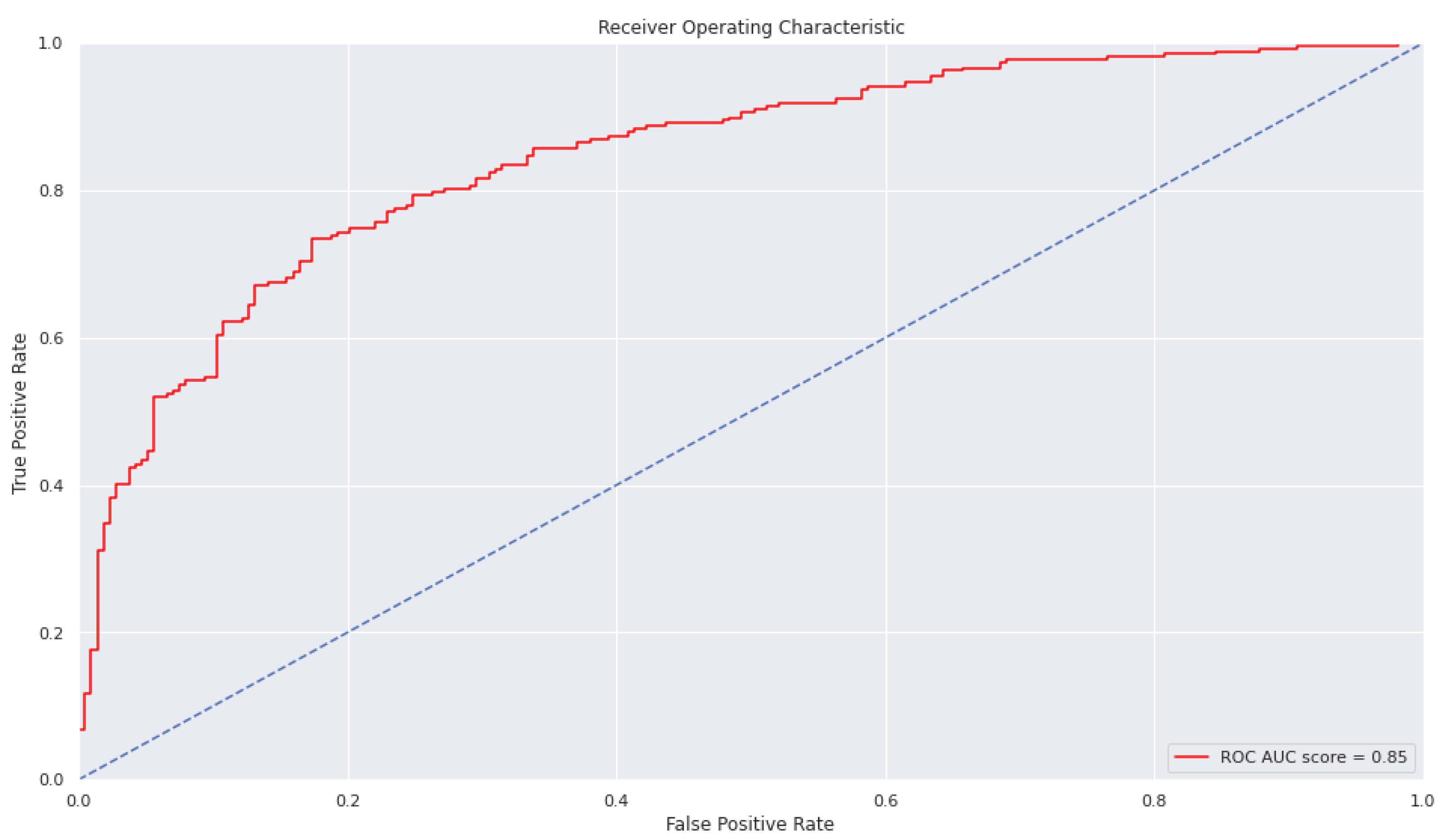
Table 3 and
Figure 4 show the results of our model. We obtained a model that performs reasonably well with the training dataset. In the Wine Quality Dataset, the accuracy of our model is 0.7667, the F1 score of the model is 0.77 and the AUC of the model is 0.85. A ROC curve is a graph showing how the diagnostic ability of a binary classifier model changes as the discrimination threshold is changed.
In the Pima Indians Diabetes Dataset, we also divided the data into a 70% training set and a 30% test set. We used 100 epochs to train the model.
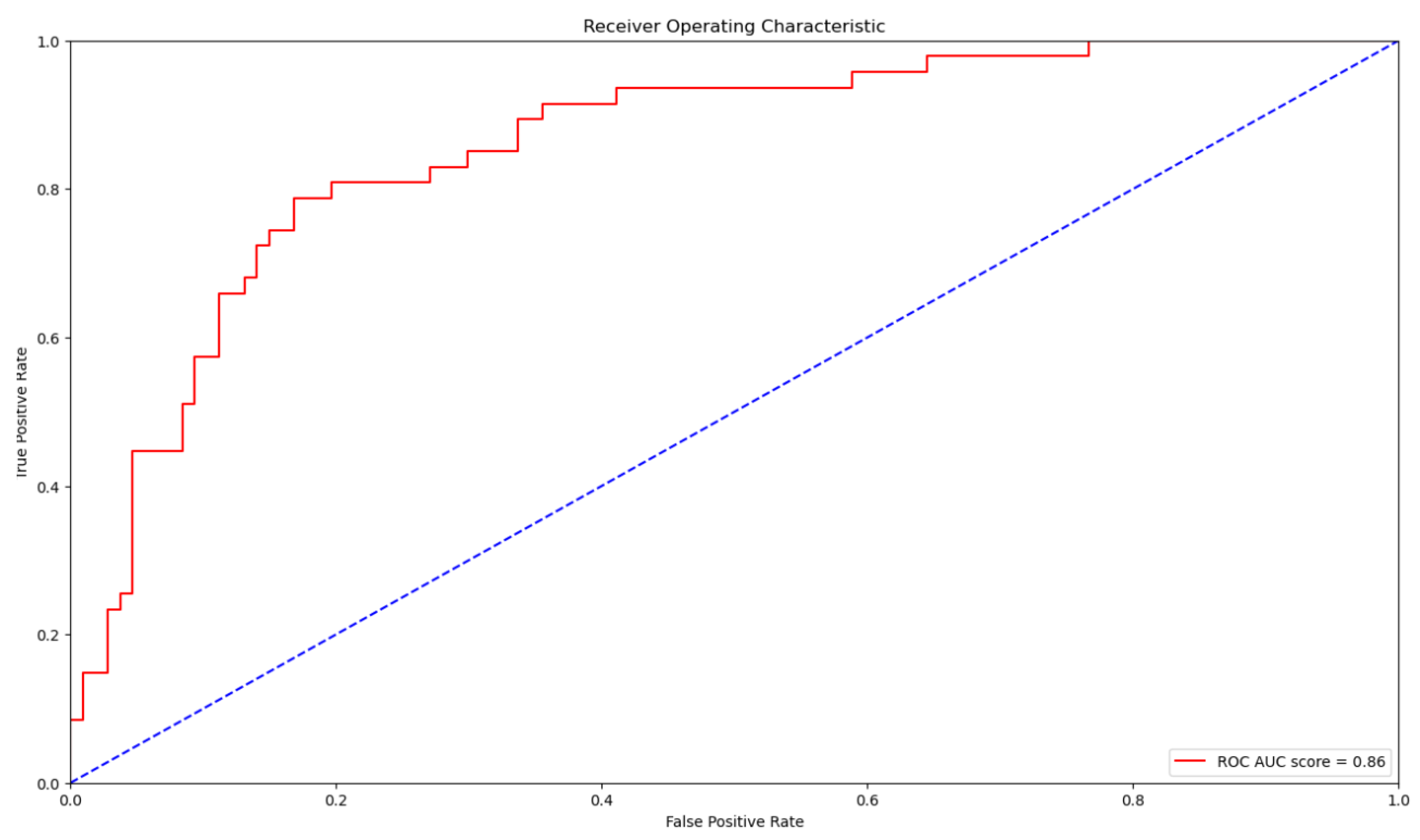
Table 4 and
Figure 5 show the results of our model. In the Pima Diabetes Dataset, the accuracy of our model is 0.8117, the F1 score of the model is 0.81 and the AUC of the model is 0.86.
4.3. The Implementation of Specific-Input LIME
We use our method to explain our black-box model. Here, we use the trained LightGBM model as our black-box model for the explanation, and we select the first data point in the tabular dataset as the instance to be explained. In our experiments, we obtain the ‘gain/split feature importance’ of the LightGBM model by calling it the ‘plot importance’ function.
In the Wine Quality Dataset, based on the feature importance in
Figure 6, we can see that the part of the graph marked with a green square is not essential when training our deep learning model. Therefore, this part of the feature is not very important for our deep learning model.
In addition, we focus on the remaining essential features (i.e., ‘alcohol’ and ‘sulphates’) in the PDP, which allows us to describe further how our model employs these features for learning. Here, we use the ‘alcohol’ feature as an example.
Figure 7 shows the PDP of the ‘alcohol’ feature.
When the value of ‘alcohol’ is more than 11.9, the impact on the model converges to a fixed value. This phenomenon shows that when learning the feature ‘alcohol’, our model groups features with values larger than 11.9 into the same category.
In the Pima Indians Diabetes Dataset, based on the feature importance in
Figure 8, The same situation occurs. The next few features in the ranking are not important to our deep learning model.
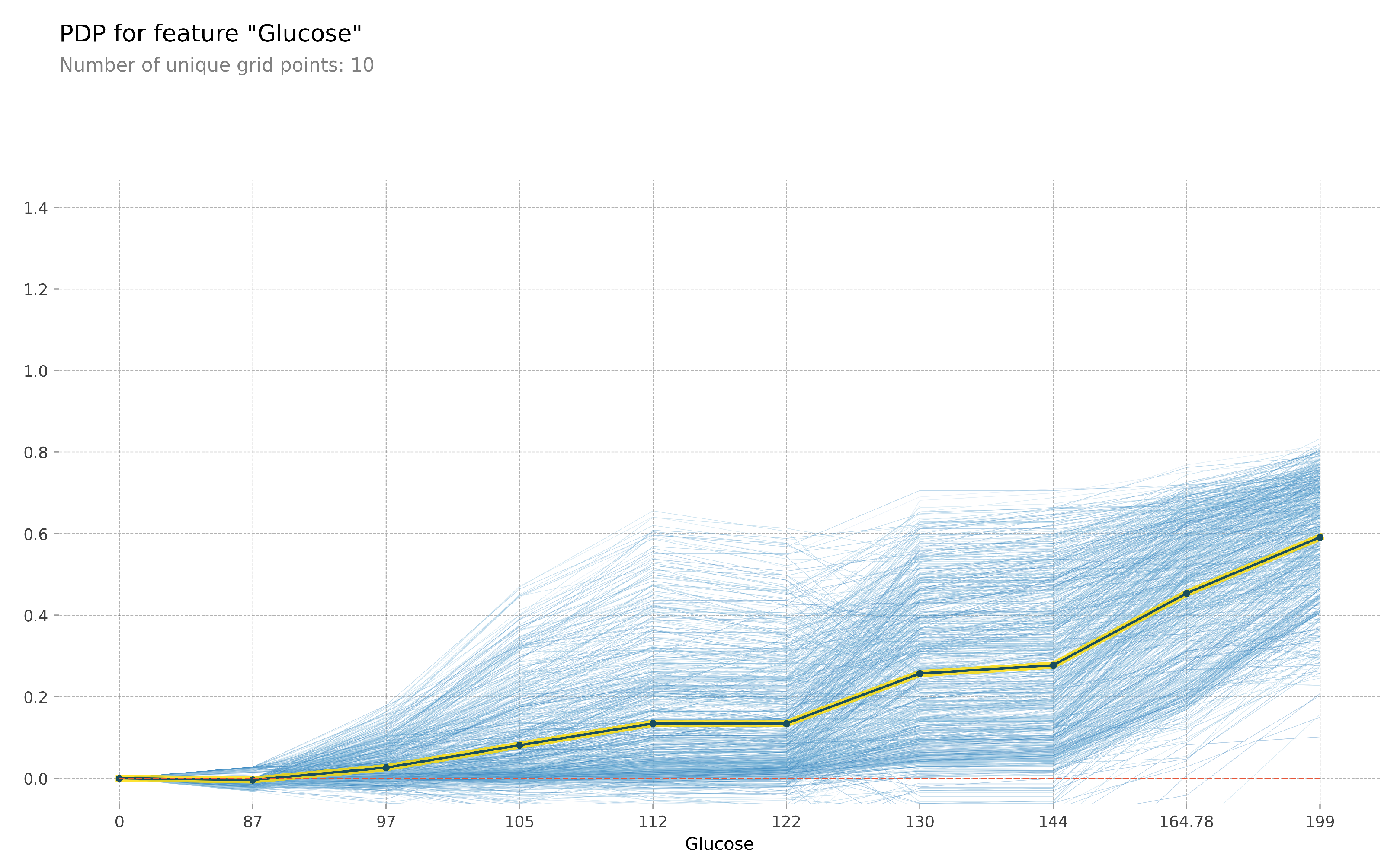
Figure 9 shows the PDP of the ‘Glucose’ feature.
4.4. The Results of Specific Input-LIME
The LIME method is used in our approach to obtain a local explanation. This explanation is mainly used to illustrate the impact of the first point in the two datasets on our model.
Figure 10 and
Figure 11 show the results of the LIME interpretation in the two datasets.
Based on the LIME method, we have added the explanation of feature importance and the PDP. Using feature importance allows us to choose which features we should look for to explain, and the PDP provides us with an interval in which the black-box model has a different importance for the features in each interval.
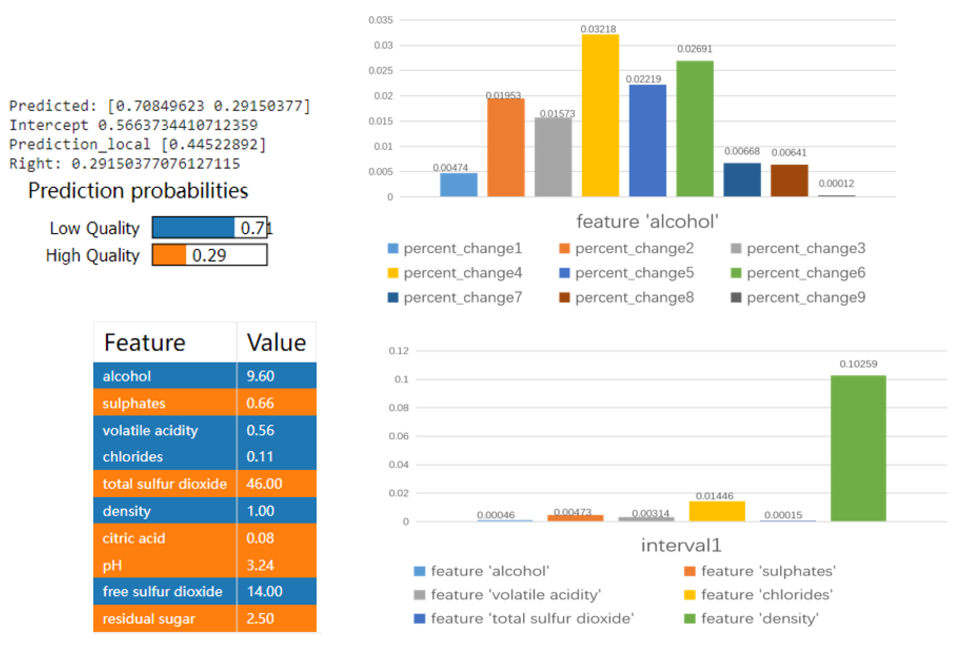
In the Wine Quality Dataset, our method allows us to expand LIME’s explanation capabilities, assuming we need to explain the feature ‘alcohol’. Using the PDP, we can see ten turning points for the feature ‘alcohol’. There are nine intervals between these ten turning points. Each interval can be considered a deep learning model learning circumstance for the value of the ‘alcohol’ feature.
We then explain each of the intervals according to ‘alcohol’. The contribution of the ‘alcohol’ feature to the model varies across these intervals. So, we replicate the data points in the dataset that belong to these intervals by finding them and assigning the value of the ‘alcohol’ feature to the mean of the interval, using the mean to obtain an average for the ‘alcohol’ feature. The averaged fake_data_frame is fed into the deep learning model as a dataset to obtain the predicted value of this model for the fake_data_frame.
Algorithm 1 shows how the feature importance and PDP values can be used to illustrate this. In reality, we are primarily interested in obtaining the variable percentage_change. This variable is usually calculated by subtracting the difference between the probability projected by the deep learning model on the original data frame and the fake_data_frame. The size of the difference represents the model’s influence when only one feature value is replaced by the mean of the interval.
The influence of the feature ‘alcohol’ on the model’s projected values in each of the nine intervals divided by the PDP is shown in
Figure 12. We can conclude from this research that ‘alcohol’ has a greater influence on the model before intervals 4 and 6 and that the ‘alcohol’ feature is regularly distributed. Our black-box model learns the ‘alcohol’ feature by giving more weight to intervals 4 and 6.
Figure 13 and
Figure 14 provide a more detailed explanation. The user can understand how the model selects features within a particular interval and how these features affect the model’s predictions.
4.5. Discussion
This paper uses specific-input LIME, a new approach to explaining models. This method is based on the original LIME method and implements a more detailed explanation. We use feature importance and PDP to compensate for the shortcomings of the LIME method. The LIME method focuses on adding random fake_data around a particular data point to obtain a boundary, whereas with the LIME method, generating fake_data will result in another interval of fake_data that exceeds the range of data learned by the original model, which interferes with the interpretability of the LIME method.
Since the main idea of this method is to combine the feature importance and the nodes in the PDP, the different feature areas are divided into different “situations” and the nodes of each fold in the PDP are segmented. For example, the point in the ‘alcohol’ PDP where the fold appears represents a shift in the situation as the model is learned. Hence, we think that the interval between the two folds in the PDP can be considered as a situation (this is just a scenario and is tentatively considered to be valid in the experiment), so there are 10 points and 9 situations in the ‘alcohol’ PDP.
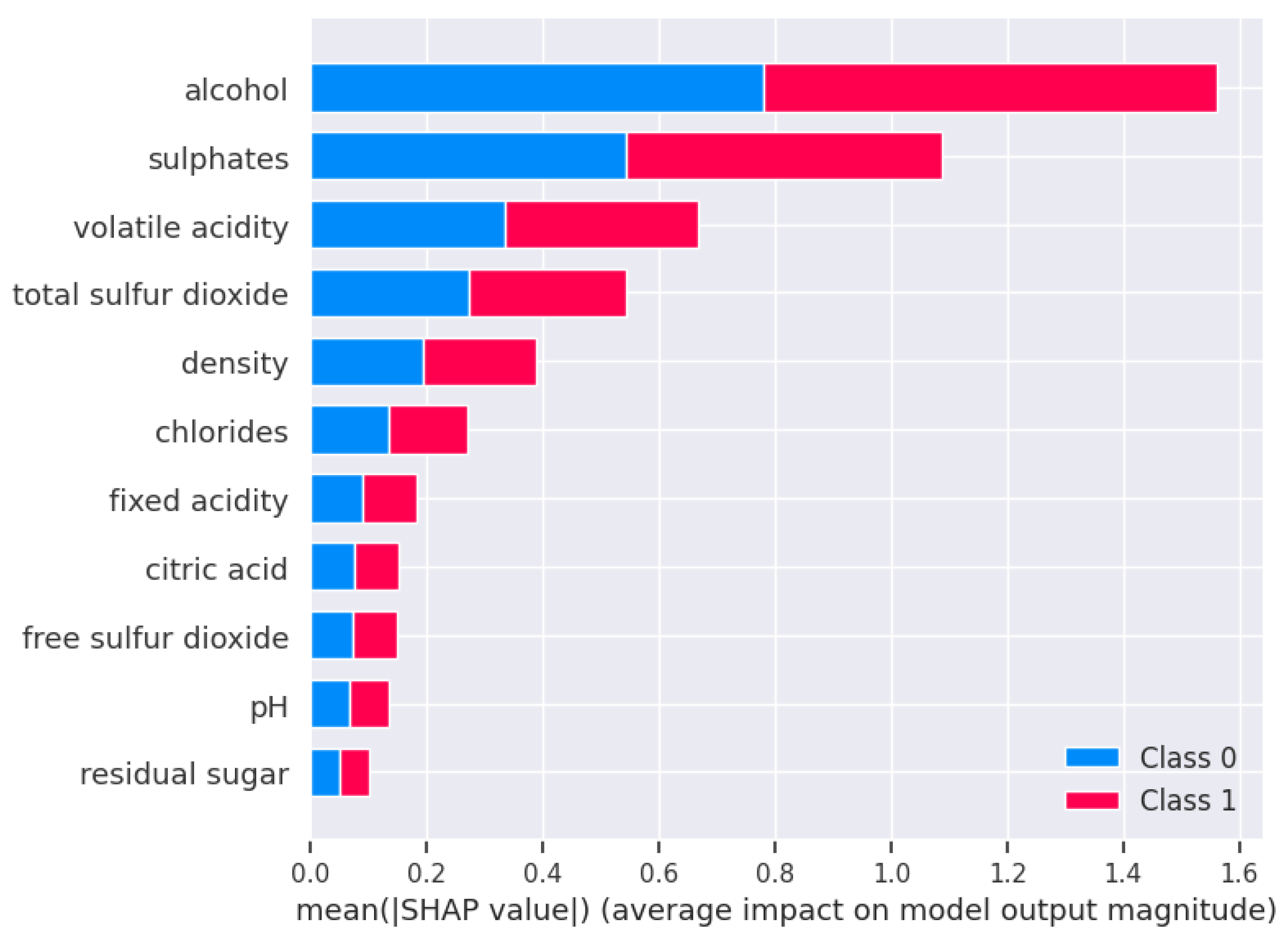
We also performed model interpretation on the same dataset using the LightGBM classifier using Shapley additive explanation (SHAP), a method proposed by Lundberg S M and Lee S I [
19] in 2017 for interpreting the predictions of machine learning models. It is based on the Shapley value in game theory, which is a fair allocation concept used to determine the contribution of each player (here understood as a feature) to the outcome of the game (in this case, the predicted outcome). The results are shown in
Figure 15 and
Figure 16. The SHAP figure is sorted from top to bottom according to the importance of the feature and the horizontal coordinate represents the SHAP value, which is the influence value. The blue colour represents the influence value of the feature on class 0 and the red colour represents the influence value of the feature on class 1. We analyse both approaches:
(1) The granularity of interpretation: Our method combines global feature importance and local feature influence (divided by turning points in the PDP), and this method provides the global influence of features in different intervals. The SHAP method, on the other hand, provides a detailed explanation of the feature contribution for each sample, as shown in the blue and red parts of
Figure 15 and
Figure 16, which allows us to understand how the prediction results for a single sample are jointly determined by the individual features. However, the LIME method can only provide local explanations [
20], i.e., explain the causes of individual predictions. In this respect, SHAP and our approach are significantly better.
(2) The accuracy of interpretation: SHAP values are calculated by a mathematical formula that assigns a fair contribution value to each feature. While our method is based on feature importance and PDP turning points, this approach can be affected by the complexity of the model and the distribution of the data, which we intend to improve later.
(3) Intuitive understanding: Our method is easier to understand because it is based on feature importance and segmentation, which are easily understood by humans. The SHAP method, on the other hand, requires an understanding of more mathematical principles.
In conclusion, both methods have advantages and suitable scenarios. When dealing with complex models, the SHAP method may be more accurate and stable, but it also has the problem of a long computation time [
21]. When focusing on the effect of a single feature on the results, the present method may be more intuitive and better suited to explain the global model behaviour.
5. Conclusions
We use the specific-input LIME method to provide the user with a more detailed explanation. Using our method, it is possible to obtain the influence of the data points that need to be explained within a particular interval, and this influence provides the user with a more intuitive explanation.
This approach can also have many applications in practice, such as in healthcare, where this combination of global and locally interpretable models can be used to explain how machine learning models predict whether a patient has a certain disease or not, and to analyse the impact of individual features on this prediction result. This can help physicians and patients to better understand the prediction results and help them make better decisions.
Although our method gives good results, it still has limitations. Since LIME, PDP, and feature importance are generated based on the perturbed data predicted by the model, they may be sensitive to the size and direction of the perturbations. If the perturbation is too large or in the wrong direction, it may lead to an unstable interpretation, so we will focus on this issue in future work. The perturbation data require the generation of a large amount of perturbation data, which can lead to high computational costs, especially for complex models or large datasets.
In future work, we will focus on parameter optimisation to reduce the computational cost and improve the robustness of this method.
Author Contributions
Conceptualization, J.A.; methodology, J.A.; software, J.A., Y.Z.; validation, J.A., Y.Z.; formal analysis, J.A., Y.Z.; investigation, J.A., Y.Z.; resources, I.J.; data curation, J.A., Y.Z.; writing—original draft preparation, J.A.; writing—review and editing, Y.Z., I.J.; visualization, J.A., Y.Z.; supervision, I.J.; project administration, I.J.; funding acquisition, I.J. All authors have read and agreed to the published version of the manuscript.
Funding
This work was supported by the Institute of Information & Communications Technology Planning & Evaluation (IITP) grant funded by the Korea government (MSIT) (No. 2020-0-00107, development of technology to automate recommendations for big data analytic models that define data characteristics and problems).
Informed Consent Statement
Informed consent was obtained from all subjects involved in the study.
Data Availability Statement
Conflicts of Interest
The funders had no role in the design of the study; in the collection, analyses, or interpretation of data; in the writing of the manuscript; or in the decision to publish the results.
Abbreviations
As there are many abbreviations of technical terms in this paper, the following appendix explains these abbreviations:
| LIME | Local interpretable model-agnostic explanations |
| XAI | Explainable artificial intelligence |
| PDP | Partial dependence plots |
| AI | Artificial intelligence |
| DNNs | Deep neural networks |
| BRL | Bayesian rule lists |
| AUC | Area under curve |
| ROC | Receiver operating characteristic curve |
| SHAP | Shapley additive explanation |
References
- Statista. Revenues from the Artificial Intelligence (AI) Market Worldwide from 2016 to 2025. 2018. Available online: https://www.statista.com/statistics/607716/worldwide-artificial-intelligence-market-revenues/ (accessed on 6 June 2018).
- Panettam, K. Gartner Top 10 Strategic Technology Trends for 2018; Smarter with Gartner; Gartner, Inc.: Stamford, CT, USA, 2017. [Google Scholar]
- Lipton, Z.C. The mythos of model interpretability: In machine learning, the concept of interpretability is both important and slippery. Queue 2018, 16, 31–57. [Google Scholar] [CrossRef]
- Doshi-Velez, F.; Kim, B. Towards a rigorous science of interpretable machine learning. arXiv 2017, arXiv:1702.08608. [Google Scholar]
- Guidotti, R.; Monreale, A.; Ruggieri, S.; Turini, F.; Giannotti, F.; Pedreschi, D. A survey of methods for explaining black box models. ACM Comput. Surv. (CSUR) 2018, 51, 1–42. [Google Scholar] [CrossRef] [Green Version]
- Letham, B.; Rudin, C.; McCormick, T.H.; Madigan, D. Interpretable classifiers using rules and bayesian analysis: Building a better stroke prediction model. Ann. Appl. Stat. 2015, 9, 1350–1371. [Google Scholar] [CrossRef]
- Caruana, R.; Lou, Y.; Gehrke, J.; Koch, P.; Sturm, M.; Elhadad, N. Intelligible models for healthcare: Predicting pneumonia risk and hospital 30-day readmission. In Proceedings of the 21th ACM SIGKDD International Conference on Knowledge Discovery and Data Mining, Sydney, Australia, 10–13 August 2015; pp. 1721–1730. [Google Scholar]
- Xu, K.; Ba, J.; Kiros, R.; Cho, K.; Courville, A.; Salakhudinov, R.; Zemel, R.; Bengio, Y. Show, attend and tell: Neural image caption generation with visual attention. In Proceedings of the 32nd International Conference on Machine Learning, Lille, France, 6–11 July 2015; pp. 2048–2057. [Google Scholar]
- Ustun, B.; Rudin, R. Supersparse linear integer models for optimized medical scoring systems. Mach. Learn. 2016, 102, 349–391. [Google Scholar] [CrossRef]
- Yang, C.; Rangarajan, A.; Ranka, S. Global model interpretation via recursive partitioning. In Proceedings of the 2018 IEEE 20th International Conference on High Performance Computing and Communications; IEEE 16th International Conference on Smart City; IEEE 4th International Conference on Data Science and Systems (HPCC/SmartCity/DSS), Exeter, UK, 28–30 June 2018; pp. 1563–1570. [Google Scholar]
- Ribeiro, M.T.; Singh, S.; Guestrin, C. “Why should i trust you?” Explaining the predictions of any classifier. In Proceedings of the 22nd ACM SIGKDD International Conference on Knowledge Discovery and Data Mining, San Francisco, CA, USA, 13–17 August 2016; pp. 1135–1144. [Google Scholar]
- Baehrens, D.; Schroeter, T.; Harmeling, S.; Kawanabe, M.; Hansen, K.; Müller, K.R. How to explain individual classification decisions. J. Mach. Learn. Res. 2010, 11, 1803–1831. [Google Scholar]
- Molnar, C. Interpretable Machine Learning; Lulu. com.: Morrisville, NC, USA, 2020. [Google Scholar]
- Zhao, X.; Huang, W.; Huang, X.; Robu, V.; Flynn, D. Baylime: Bayesian local interpretable model-agnostic explanations. In Uncertainty in Artificial Intelligence; PMLR: London, UK, 2021; pp. 887–896. [Google Scholar]
- Friedman, J.H. Greedy function approximation: A gradient boosting machine. Ann. Stat. 2001, 29, 1189–1232. [Google Scholar] [CrossRef]
- Cortez, P.; Cerdeira, A.; Almeida, F.; Matos, T.; Reis, J. Modeling wine preferences by data mining from physicochemical properties. Decis. Support Syst. 2009, 47, 547–553. [Google Scholar] [CrossRef] [Green Version]
- Vaishali, R.; Sasikala, R.; Ramasubbareddy, S.; Remya, S.; Nalluri, S. Genetic algorithm based feature selection and MOE Fuzzy classification algorithm on Pima Indians Diabetes dataset. In Proceedings of the International Conference on Computing Networking and Informatics (ICCNI), Lagos, Nigeria, 29–31 October 2017; pp. 1–5. [Google Scholar]
- Wang, C.; Wu, Q.; Weimer, M.; Zhu, E. FLAML: A fast and lightweight automl library. In Proceedings of the Machine Learning and Systems, Santa Clara, CA, USA, 4–7 April 2021; pp. 434–447. [Google Scholar]
- Lundberg, S.M.; Lee, S.I. A unified approach to interpreting model predictions. In Proceedings of the Advances in Neural Information Processing Systems, Long Beach, CA, USA, 4–9 December 2017; Volume 30. [Google Scholar]
- Toğaçar, M.; Muzoğlu, N.; Ergen, B.; Yarman, B.S.B.; Halefoğlu, A.M. Detection of COVID-19 findings by the local interpretable model-agnostic explanations method of types-based activations extracted from CNNs. Biomed. Signal Process. Control 2022, 71, 103128. [Google Scholar] [CrossRef] [PubMed]
- Rajapaksha, D.; Bergmeir, C. LImref: Local interpretable model agnostic rule-based explanations for forecasting, with an application to electricity smart meter data. Proc. AAAI Conf. Artif. Intell. 2022, 36, 12098–12107. [Google Scholar] [CrossRef]
Figure 1.
LIME algorithm for tabular data.
Figure 1.
LIME algorithm for tabular data.
Figure 2.
Explanation of the example x = 1.6 prediction.
Figure 2.
Explanation of the example x = 1.6 prediction.
Figure 3.
The architecture of specific-input LIME.
Figure 3.
The architecture of specific-input LIME.
Figure 4.
AUC-ROC curve of the Wine Quality Dataset.
Figure 4.
AUC-ROC curve of the Wine Quality Dataset.
Figure 5.
AUC-ROC curve of the Pima Indians Diabetes Dataset.
Figure 5.
AUC-ROC curve of the Pima Indians Diabetes Dataset.
Figure 6.
The feature importance of our black-box model in the Wine Quality Dataset.
Figure 6.
The feature importance of our black-box model in the Wine Quality Dataset.
Figure 7.
The PDP plot of ‘alcohol’ feature.
Figure 7.
The PDP plot of ‘alcohol’ feature.
Figure 8.
The feature importance of our black-box model in the Pima Indians Diabetes Dataset.
Figure 8.
The feature importance of our black-box model in the Pima Indians Diabetes Dataset.
Figure 9.
The PDP plot of ‘Glucose’ feature.
Figure 9.
The PDP plot of ‘Glucose’ feature.
Figure 10.
The result of the LIME method in the Wine Quality Dataset.
Figure 10.
The result of the LIME method in the Wine Quality Dataset.
Figure 11.
The result of the LIME method in the Pima Indians Diabetes Dataset.
Figure 11.
The result of the LIME method in the Pima Indians Diabetes Dataset.
Figure 12.
The result of explaining the feature ‘alcohol’ using percent_change.
Figure 12.
The result of explaining the feature ‘alcohol’ using percent_change.
Figure 13.
The explanation of using specific-input LIME for the first data point in the Wine Quality Dataset.
Figure 13.
The explanation of using specific-input LIME for the first data point in the Wine Quality Dataset.
Figure 14.
The explanation of using specific-input LIME for the first data point in the Pima Indians Diabetes Dataset.
Figure 14.
The explanation of using specific-input LIME for the first data point in the Pima Indians Diabetes Dataset.
Figure 15.
The explanation of using SHAP in the Pima Indians Diabetes Dataset.
Figure 15.
The explanation of using SHAP in the Pima Indians Diabetes Dataset.
Figure 16.
The explanation of using SHAP in the Wine Quality Dataset.
Figure 16.
The explanation of using SHAP in the Wine Quality Dataset.
Table 1.
Data description.
Table 1.
Data description.
| Dataset | Wine Quality Dataset | Pima Indians Diabetes Dataset |
|---|
| Dataset Characteristics: | Multivariate | Multivariate |
| Area: | Business | Medical research |
| Associated Tasks: | Classification | Classification |
| Number of Instances: | 4898 | 768 |
| Number of Attributes: | 11 | 8 |
| Missing Values: | N/A | N/A |
Table 2.
Model parameters.
Table 2.
Model parameters.
| Model: | LightGBM Classifier |
|---|
| Num_leaves: | 27 |
| Min_child_samples: | 7 |
| Learining_rate: | 0.1400468994301556 |
| Log_max_bin: | 10 |
| Colsample_bytree: | 0.9159235947614908 |
| Reg_alphg: | 0.0009765625 |
| Reg_lambda: | 3.136860108634179 |
Table 3.
The Wine Quality Dataset model performance.
Table 3.
The Wine Quality Dataset model performance.
| | Precision | Recall | F1-Score | Accuracy |
|---|
| Low Quality: | 0.73 | 0.75 | 0.74 | 0.7667 |
| High Quality: | 0.80 | 0.78 | 0.79 | 0.7667 |
| Macro avg: | 0.76 | 0.77 | 0.76 | 0.7667 |
| Weighted avg: | 0.77 | 0.77 | 0.77 | 0.7667 |
Table 4.
The Pima Indians Diabetes Dataset model performance.
Table 4.
The Pima Indians Diabetes Dataset model performance.
| | Precision | Recall | F1-Score | Accuracy |
|---|
| 0: | 0.88 | 0.85 | 0.86 | 0.8117 |
| 1: | 0.68 | 0.72 | 0.70 | 0.8117 |
| Macro avg: | 0.78 | 0.79 | 0.78 | 0.8117 |
| Weighted avg: | 0.82 | 0.81 | 0.81 | 0.8117 |
| Disclaimer/Publisher’s Note: The statements, opinions and data contained in all publications are solely those of the individual author(s) and contributor(s) and not of MDPI and/or the editor(s). MDPI and/or the editor(s) disclaim responsibility for any injury to people or property resulting from any ideas, methods, instructions or products referred to in the content. |
© 2023 by the authors. Licensee MDPI, Basel, Switzerland. This article is an open access article distributed under the terms and conditions of the Creative Commons Attribution (CC BY) license (https://creativecommons.org/licenses/by/4.0/).


